diminishing value of the derivative of the commonly used activation ... Backpropagation updates the weights iteratively to map a set of input vectors (X. 1. ,X. 2. ,â¦,X p. ) to a set of .... Simulation results show that arctangent activation function.
A Note on Activation Function in Multilayer Feedforward Learning Joarder Kamruzzaman Faculty of Information technology Monash University, Gippsland Campus Victoria-3842, Australia
S.M.Aziz School of Electrical & Information Eng. University of South Australia Mawson Lakes, SA 5095, Australia
Abstract: - Multilayer feedforward network trained by Backpropagation algorithm suffers from slow learning speed. One of the reasons of slow convergence is the diminishing value of the derivative of the commonly used activation functions as the nodes approaches saturated values. In this paper, we present a new activation function to accelerate Backpropagation learning. A comparison among the commonly used activation functions, recently proposed logarithmic function and proposed activation function shows accelerated convergence with the proposed one. This activation function can be used in conjunction with other techniques to further accelerate the learning speed or reduce the chance of being trapped in local minima.
function [2-4], (ii) dynamic variation of learning rate and momentum [5-10], (iii) selection of better activation function of the neurons [11]. One of reasons of slow convergence in Backpropagation is the sigmoid activation function used in hidden and output layer units. In [11], Bilski proposed a new logarithmic activation function in lieu of sigmoid activation function. In this paper, we present an inverse tangent activation function for hidden and output units. Simulation results with different categories of problems show improved learning speed when this activation function is used.
Simulation using this activation function shows improvement in learning speed compared with other commonly used functions and a new activation function proposed in [11]. This function may also be used in other multilayer feedforward training algorithms.
In the following, we present a brief description of Backpropagation learning and commonly used activation functions. We also propose a new activation function in order to accelerate the learning process.
2. BP LEARNING AND ACTIVATION FUNCTION
2.1 BP learning Key words: Neural network, backpropagation learning, activation function, learning speed.
1. INTRODUCTION Backpropagation (BP) is the most widely used algorithm for training multilayer feedforward neural network [1]. The algorithm uses gradient descent technique to adjust the connection weights between neurons in order to minimize the system error between the actual output and desired target output. One of the major drawbacks of Backpropagation learning is its slow convergence. New applications of neural networks in different areas like data mining, knowledge discovery, intelligent agents etc. demand faster learning. Different modifications of standard Backpropagation algorithm have been proposed to improve convergence [2-11]. Approaches to improve convergence speed include, (i) selection of better cost
0-7803-7278-6/02/$10.00 ©2002 IEEE
Backpropagation updates the weights iteratively to map a set of input vectors (X1,X2,…,Xp) to a set of corresponding output vectors (Y1,Y2,…,Yp). The input is presented to the network and multiplied by the weights. All the weighted inputs fed to each neuron in the upper layer are summed up, and produce output governed by the following equation.
okp = f (net kp ) = f (∑ ω kj o jp +θ k )
(1)
j
where
okp is
the output of neuron ‘k’ for p-th pattern,
o jp is the output of neuron ‘j’ at the lower layer, ω kj is the weight between the neurons ‘k’ and ‘j’. net kp is the net input feeding to neuron ‘k’ from the lower layer for pattern
‘p’,
θ k is the bias for unit ‘k’ and f (.)
is the activation
function of the neurons.
The cost function to be minimized in Backpropagation is the sum of squared error measured at the output layer and defined as
E=
2 1 ∑ ∑ (t kp − o kp) 2 p k
where
t kp
and
okp
(2)
are the target and actual outputs of
neuron ‘k’ for pattern ‘p’. Backpropagation uses the steepest descent technique for changing weights in order to minimize the cost function of Equ. (2). The weight update at t-th iteration is governed by the following equation.
∆ω (t ) = − η
∂E +α ∆ω (t − 1) ∂ω (t )
(3)
where η and α are the learning rate and momentum factor respectively. The derivative of the error function E with respect to weight ω in the above equation is proportional to the first derivative of the activation function, i.e.,
∂E ∝ f ′(net ) ∂ω
(4)
The magnitude of the first derivative of the activation function is one of the main reasons that contribute to the slow convergence of Backpropagation learning. When the actual output okp approaches to either of the extreme values, namely 0 or ± 1, the value of the derivative diminishes. This will produce very small back propagated error signal resulting in very small weight change. Thus, the output can be maximally wrong without producing any significant weight change. The algorithm may then be trapped into local minima. Consequently, the learning process and weight adjustment will be very slow or even suppressed. 2.2 Commonly used activation function The activation function commonly used in Backpropagation learning is either sigmoid (fs) or tanget hyperbolic (fth), and expressed as
o = f s (net ) =
1 , and 1 + e − net
0-7803-7278-6/02/$10.00 ©2002 IEEE
o = f th (net ) =
e net − e − net e net + e − net
Their first derivatives are calculated as
f ′s (net ) = o (1 − o) , and f ′th (net ) = (1 + o)(1 − o) Above expression shows that the derivatives have diminishing values when the output approaches either of the extreme values. 2.3 Recently used activation function Recently logarithmic transfer function have been proposed in [11] with an idea to have lager derivatives as the output reaches extreme values and is expressed as follows,
ln(net + 1) o = f l (net ) = − ln(− net + 1)
net ≥ 0 net < 0
The derivative of the above function is expressed as
f ′l (net ) =
1 1 + net
The above activation functions and their first derivatives are shown in Fig. 1 and Fig. 2, respectively. 2.2 Proposed activation function Fig. 2 shows that the derivative of logarithmic function is higher than that of the others near the saturation region, i.e., output approaching ±1 or 0 in case of sigmoid function. However, a too high value of the derivative at the later stage of learning may cause inappropriately large weight changes causing oscillation. Here we propose inverse tangent activation whose derivative is larger than the sigmoid or tangent hyperbolic function but smaller than logarithmic when output approaches ±1. The function is expressed as
o = f (net ) = arctan(net ) it Fig. 1 and Fig. 2 show this function and its derivative respectively.
Sigmoid Tangent hyperbolic Logarithm
literatures. The second is a character recognition problem chosen for neural network’s suitability in character recognition applications. The third is the Wine data set available at machine learning database [12]. The forth is an Encoder problem also found in many literature [12-14].
2 1.5 1
Arctangent
3.1
Output
0.5 0
-6
-4
-2
0
2
4
6
-0.5 -1 -1.5 -2 Net Input
Fig. 1: Different activation functions.
XOR Problem
A 2-2-1 network (two inputs, two hidden and one output neuron) network was trained using Backpropagation learning with different activation functions. In each case the network was initialized with small random values. Investigation was done with different values of η, α and training was continued until sumsquared error reduces to 0.01. Twenty trials with different initial weights were carried out and the average training cycle required to train the network is presented in Table 1. Table 1: Comparison of training epochs required to learn XOR problem.
1.2
Sigmoid
η
Tangent Hyperbolic Logarithmic
Derivative
Arctangent
1 0.8
0.1
0.6
0.3
0.4 0.2
-6
-4
-2
0 Net 0 Input
0.5 2
4
6
Fig. 2: Derivatives of the activation functions shown in Fig.1
α 0.0 0.3 0.6 0.8 0.0 0.3 0.6 0.8 0.0 0.3 0.5 0.8
Sigmoid Tangent hyperbolic 19881 2924 11876 2015 6457 1027 3684 749 3721 1107 2853 609 1688 398 868 307 6852 463 1629 352 1173 193 572 177
Logarithmic 1534 1234 655 378 560 311 211 141 247 162 95 79
Arctangent 745 454 238 120 185 132 67 44 136 38 28 24
Simulation results show that arctangent activation function improves the learning speed in standard Backpropagation learning. 3.2 Character Recognition Problem
3. SIMULATION RESULTS In order to investigate the convergence speed of Backpropagation learning with different activation functions mentioned above, simulations are carried out with different types of problems. Since no analytical techniques are available to study the learning speed Backpropagation algorithm, simulation with different problems and comparison is the usually adopted means to evaluate the effectiveness of a modification. In the present work, investigation has been done with four different problems. The first one is the XOR problem which is treated as a benchmark problem in many neural network 0-7803-7278-6/02/$10.00 ©2002 IEEE
Experiment was conducted with ten numeric digits (0~9). Each digit consists of 16×16 binary pixel. Target vectors corresponding to each input was a locally represented one, i.e., only one neuron at the output layer was active and the rest were zero. The network had 256 input neurons and ten output neurons to represent ten categories. A 256-9-10 network was trained using different activation functions. The networks were trained with different values of η and α. For each set of η and α, 50 trails were made. As a stopping criteria we used
max t kp − okp ≤ γ for all iterations in epoch
where γ is arbitrarily taken chosen threshold and was set 0.1 in this experiment. Simulation results showing the average training cycles of 50 trials are presented in Table 2. Table 2: Comparison of training epochs required to learn character recognition problem η 0.05
0.075 0.1
α 0.3 0.4 0.5 0.3 0.4 0.5 0.3 0.4 0.5
Sigmoid Tangent hyperbolic 950 308 823 254 670 225 708 187 488 179 401 135 440 160 377 117 304 107
Logarithmic 100 96 86 81 63 61 70 57 60
Arctangent 93 75 73 69 52 57 63 57 54
3.4 The 10-5-10 Encoder Problem The encoder problem has been largely described in [1214]. The task is to learn an auto association between 10 binary input/output patterns. The network consists of 10 neurons in both the input and the output layer, and a hidden layer 5 neurons. Table 4 summarizes the result of realizing this task with different activation function taking the average epochs of 30 successful trials. Results show that for some of the learning rate and momentum values logarithmic activation causes slower learning. This is because these parameter values coupled with the higher value of the derivative causes oscillation in the learning process resulting in slow convergence. However, use of arctangent activation function yields better learning speed. Table 4: Comparison of training epochs required to learn the encoder problem. η
3.3 Learning Iris data Set Iris plant database is one of the best-known data set found in various literature [12]. The data set contains 3 classes of 50 instances each, where each class refers to a type of iris plant. One class is linearly separable from the other two; the latter are not linearly separable from each other. Each instance has four inputs regarding the iris plant. This is a much harder problem compared to the previous two to learn with neural network. We attempted to train the data set with a 4-20-3 network. Stopping criteria is the same as the previous problem with γ set to 0.2. Our experience shows that BP with sigmoid function could not learn the problem even after 150000 iteration in 50 trials. With other activation functions, learning converged only with small value of η and α. Table 3 shows average training epochs of the successful trials and the number of successful trials out of 50 attempted trials. Results show that logarithmic and arctangent activation functions are able to learn the problem with higher successful trials in a relatively small number of epochs. Table 3: Comparison of training epochs required to learn Iris plant recognition problem. The second entry in each row indicates the number of successful trials. η 0.010
0.015
α 0.0 0.1 0.2 0.0 0.1 0.2
Tangent Logarithmic hyperbolic 63517, 19 54596 ,31 55956, 22 50936, 33 45437, 22 41654, 37 53279, 23 44376, 34 48934, 22 43891, 35 40765, 20 38249, 31
0-7803-7278-6/02/$10.00 ©2002 IEEE
Arctangent 53231, 35 49735, 33 37105, 38 42975, 37 41348, 39 35189, 33
0.1
0.2 0.3
α 0.1 0.2 0.3 0.1 0.2 0.3 0.1 0.2 0.3
Sigmoid Tangent hyperbolic 1490 104 1312 77 1042 81 765 91 726 55 688 39 540 88 512 79 498 72
Logarithmic 95 82 88 88 57 55 70 93 97
Arctangent 75 70 68 50 47 32 63 57 54
4. CONCLUSION In this paper, a comparative study of Backpropagation learning with different activation functions has been proposed. The newly proposed activation function shows considerable acceleration of learning speed in comparison with other commonly used and recently proposed logarithmic activation function. Use of this activation function with other techniques like combined iterative method [9] or generalized backpropagation [10] can further accelerate the convergence and reduce the chance of being trapped in local minima. 5. REFERENCES [1] D.E Rumelhart, J.L. McClelland and the PDP research group, Parallel Distributed Processing, vol. 1, MIT Press, 1986. [2] M.J. Holt, “Comparison of generalization in multiplayer perceptron with log-likelihood and leastsquares cost function,” in Proc. 11th IAPR, Int. Conf.
[3] [4] [5] [6] [7]
[8]
On pattern Recognition, The Netherlands, II, pp. 1720, 1992. M. Ahmad and F.M.A Salam, “Supervised learning using the cauchy energy function,” in Proc. Int. Conf. on Fuzzy Logic and Neural Network, 1992. A. Ooyen and B. Neinhuis, “Improving the convergence of the back-propagation algorithm,” Neural Networks, vol. 5, pp. 465-471, 1992. R.A. Jacobs, “Increased rates of convergence through learning rate adaptation,” Neural Networks, vol. 1, pp. 295-307, 1988. M.K. Weir, “A method for self determination of adaptive learning rates in back propagation,” Neural Networks, vol. 4, pp. 371-379, 1991. X.H. Yu et al, “Acceleration of backpropagation learning using optimised learning rate and momentum,” Electronic Letters, vol. 29, no.14, pp. 1288-1289, 1993. J. Kamruzzaman, “Fast training of multilayered feedforward neural networks,” in Proc. 3rd JapanAustralia Joint Workshop on Intelligent and Evolutionary Systems, Australia, pp. 78-85, 1999.
0-7803-7278-6/02/$10.00 ©2002 IEEE
[9] B. Verma , “Fast training of multilayered perceptrons,” IEEE Trans. on Neural Networks, vol. 8, no. 6, 1997 [10] S.C. Ng et. al., “Fast convergent generalized backpropagation algorithm with constant learning rate,” Neural Processing Letters, vol. 9, pp. 13-23, 1999. [11] J. Bilski, “The Backpropagation learning with logarithmic transfer function,” in Proc. 5th Conf. On Neural Networks and Soft Computing, Poland, pp. 7176, June 2000. [12] UCI repository of machine learning databases, http://www.isc.uci.edu/pub/machine-learningdatabases. [13] S.E. Fahlman, “An empirical study of learning speed in backpropagation networks,” Technical report, CMU-CS-88-162, 1988. [14] M. Reidmiller and H. Braun, “A direct adaptive method for faster Backpropagation learning: The EPROP algorithm,” in Proc. IEEE International Conference on Neural Networks, San Francisco, CA, pp. 586-591, 1993.