of the transducer. Thus, the direct instrument output can be used to represent ground acceleration up to about 5 to 15 cps. If information on higher frequencies is ...
Bulletin of the Seismological Society of America. Vol. 62, No. 1, pp. 401-409. February, 1972
A N O T E ON C O R R E C T I O N OF S T R O N G - M O T I O N A C C E L E R O G R A M S FOR I N S T R U M E N T RESPONSE BY M . D . TRIFUNAC ABSTRACT
Two methods for accelerometer instrument correction are described: (1) a direct numerical differentiation of recorded accelerograms from which high-frequency digitization errors have been filtered out and (2) an ideal "mathematical accelerometer" with a natural frequency significantly higher than the natural frequency of the recording instrument. Although both methods give good results, the first one is recommended for standard use.
INTRODUCTION
To record ground acceleration, the relative response of a single-degree-of-freedom viscously-damped oscillator is usually employed. The natural frequency of such a transducer is between 10 and 30 cps, while the equivalent viscous damping is about 60 per cent of critical. The recorded relative instrument response approximates accurately the ground acceleration in the frequency range from 0 cps to about ½ to ¼ of the natural frequency of the transducer. Thus, the direct instrument output can be used to represent ground acceleration up to about 5 to 15 cps. If information on higher frequencies is required, instrument correction of the recorded accelerogram must be performed. Modern computational methods in the dynamics of structures now require the accurate high-frequency part of the accelerogram, in order to determine the response of the higher modes of vibration. Detailed studies of earthquake source parameters and especially the studies aimed at the determination of the size of the earthquake dislocation surface and the effective stress call for the maximum possible accuracy in the high-frequency end of the Fourier amplitude spectrum of ground acceleration. Unlike the baseline correction of accelerograms (Trifunac 1970) considered by many investigators, the instrument correction problem was studied by only a few. Jenschke and Penzien (1964) proposed an approximate method for the accelerograph instrument correction in response-spectrum calculations. Their method was based on a numerical approximation of the first derivative of an accelerograph transducer's recorded relative response, whereas McLennan (1969) derived an exact method to correct for accelerometer error in the dynamic response calculations. The disadvantage in both of these methods was that they were designed to correct the response spectra and not the recorded accelerogram that serves as the basic input for all computations. In this paper, we present two different types of accelerometer instrument corrections. The first method, based on our previous work (Trifunac and Hudson 1970), uses direct numerical differentiation of an instrument response. This differentiation is performed after high-frequency digitization errors are filtered out from digitized data. The second method is the extension of McLennan's (1969) approach. It consists of computing the response of a high-frequency oscillator that has a natural frequency significantly higher than the accelerometer frequency. INSTRUMENT CORRECTION
From Figure 1, it may be concluded that for the natural frequencies of acceleration transducers between 10 and 30 cps (~o. = 60 to 200 rad/sec) the instrument response may be taken to represent ground accelerations up to frequencies of about 5 to 10 cps, 401
402
BULLETIN OF T H E SEISMOLOGICAL SOCIETY OF AMERICA
respectively. To accurately recover higher frequencies, an instrument correction must be performed. In this work, we will neglect errors resulting from imperfections in the transducer design. This is permissible because the routine optical-mechanical digitization process does THE SINGLE-DEGREE-OF-FREEDOM SYSTEM 5 i
~ ~"
4
O
-I
l
~ O
I
!=====i==:==~
3
0d/COn_.l~_ 2
(a)
,80
¢'. i.. ~: o.,~_.¢-~ L/z~--
~120
/~
o ~_ 1
i-
~ =
nO - 90
03
>= o and
~o_o-o-~Xa(nAt)+ ~Xa(n'-Z~t)l] "~"
or
'~
~
I~;=0.707 I
FIG. 4.
distributed over the filtering interval of I sec, the resulting f lter transfer function is as in Figure 5. For this particular example, we chose to analyze a typical case for which the characteristic high-frequency cutoff is determined by the digitization noise level, far beyond the instrument natural frequency, here chosen as 1 cps. We believe that such an example TRANSFER FUNCTION FOR ORMSBY FILTER 1.0
Z O I.c) z LL n" 0.5 uJ LL CO Z