[BGHK95] Hans L. Bodlaender, John R. Gilbert, HjбlmtÑr Hafsteinsson, and Ton Kloks. ... 99] B. Cabon, S. de Givry, L. Lobjois, T. Schiex, and J.P. Warners.
A note on CSP graph parameters T. Schiex July 1999 Abstract Several graph parameters such as induced width, minimum maximum clique size of a chordal completion, k-tree number, bandwidth, front length or minimum pseudo-tree height are available in the CSP community to bound the complexity of specific CSP instances using dedicated algorithms. After an introduction to the main algorithms that can exploit these parameters, we try to exhaustively review existing parameters and the relations that may exist between then. In the process we exhibit some missing relations. Several existing results, both old results and recent results from graph theory and Cholesky matrix factorization technology [BGHK95] allow us to give a very dense map of relations between these parameters. These results strongly relate several existing algorithms and answer some questions which were considered as open in the CSP community.
Warning:
this document is a working paper. Some sections may be incomplete or currently being worked out ([GJC94] degree of cyclicity not considered yet, complexity section unfinished. . . )
1
Introduction
The Constraint Satisfaction Problem(CSP) is an NP-hard problem which is now widely used in Artificial Intelligence to represent numerous important combinatorial problems such as scheduling, diagnosis, VLSI design, decision-support. . . A CSP is simply defined by a set of variables to which values must be assigned without violating constraints that specify forbidden value combinations. In the worst-case, a CSP algorithm is typically exponential in the number of variables. However, for some specifics classes of instances, improved bounds are provided by algorithms that exploit the structure of the constraint graph of these instances. An interesting property of these algorithms (most are dynamic programming like algorithms) is that they can be easily extended to cope with extensions of CSP such as Valued CSP [SFV95] or Semiring CSP [BMR95] or more generally with constraint optimization problems [BB72, DDP90, SS88]. Although this is our main motivation, this paper will stick to classical CSP, considering that the extension of these algorithms to optimization is not the hardest part and has already been tackled in several cases. The constraint graph of a CSP is defined by representing each variable with a vertex and each constraint by an edge connecting the restricted variable (when constraints are not necessarily binary, a constraint hyper-graph can be defined accordingly). The most famous parameter is probably the minimum width of the graph [Fre82] which, as a side-effect, defines one the most important polynomial class of CSP: CSP whose minimum width is one i.e., whose graph is a forest. The next section, after a small review of the main algorithms (along with their applicability to valued CSP) will give the definition of most existing bounding parameters for CSP along as several other parameters. Then, the following section gives all the relationships that could either be found or proved between these parameters. For several of these, the relationship is usually considered as folklore in graph theory. For some others, the relationship connects traditional CSP parameters with bounding parameters used eg. in parallel Cholesky matrix factorization, which enables us to immediately catch up with the state of the art in this field. Finally, a few missing relationships are proved in this paper. These relationships give a better understanding of existing procedures and bring to light obvious connections between existing methods. They also show how tightly these parameters depend one on the other.
1
Section 5 consider the complexity of computing these parameters. Some problems which were considered as open in the CSP community can be shown to be NP-complete using the previous relationships and some recent results on approximating these parameters are also available. Finally, to give to these parameters some practical flavor, we present upper bounds on some of these parameters computed on real instances obtained by [KvHK99] and [VLS96]. The results show that graph parameters can have a practical significance which has been largely ignored.
2
Algorithms
A binary CSP is defined by set of n variables V and a set of e constraints C involving pair of variables. Variable domains are supposed to be finite, d being the size of the largest domain. The constraint graph G of a binary CSP is the graph (V; E ) where each vertex is a variable and each edge represent one constraint, connecting the pair of variables involved in this constraint. In the sequel, we always assume that the graph of the CSP is connected. When non binary constraints exists, the graph becomes an hyper-graph. In this case we will implicitly use the 2-section of the hyper graph as the graph of the CSP. The 2-section of an hypergraph is obtained by replacing each hyper-edge by a complete graph over the vertices in the hyperedge. Given a graph G(V; E ), with n vertices, an ordering � is a one-to-one mapping from V to f1; : : : ; ng: �(v) is the position of vertex v in the ordering �. We will note �0 (i) the ith vertex in the ordering (i.e., �0 = � 1 ). The subgraph induced by a subset of vertices W � V and more generally the subproblem induced by a subset of variables W is noted GW .
2.1 Non serial dynamic programming or elimination algorithms The first class of algorithm that exploits structural parameters can be covered under the name of non serial dynamic programming algorithms [BB72]. Very roughly, in the CSP case, these dynamic programming algorithms work as follow : 1. choose a subproblem (a CSP defined by a partial subgraph of the problem) and solve it completely, collecting all solutions (using eg. a backtrack tree search algorithm). 2. mark the subproblem as solved. 3. project the set of solutions obtained previously on the variables of the subproblem which are shared with the yet unsolved part of the CSP. The set of these variables define the separator of the subproblem. This add an unsolved induced constraint to the CSP (if a constraint already exists on these variables, compute their intersection). 4. proceed until no unsolved constraint remains. Note that in order to progress, the subproblem chosen in step 1 must be so that its resolution in step 2 strictly simplifies the problem. A condition that suffices to guarantee this is that each subproblem must include at least one variable with all the constraints that involve it. The number of variables in the unsolved part will then be always strictly smaller than initially. When this type of subproblem is used at each step (choosing one variable), the algorithm is called variable elimination. Other choices are possible eg., one may choose to eliminate more than one variable in one step. Quite obviously, the consistency of the final problem obtained is equivalent to the consistency of the original problem since only the restrictions induced by a subproblem on the rest of the problem have been added in the induced constraint. It is actually easy to build any solution to the original problem by proceeding in a reverse order: one starts with a solution of the last subproblem and extend it consistently to the next subproblem... There will be no backtrack since all the combinations that could not lead to a solution have been explicitly forbidden by the induced constraints (in some sense, the problem has been made “directionally” globally consistent). In my knowledge, the first general dynamic programming algorithm for CSP is Seidel’s invasion algorithm [Sei81]. Rather than presenting Seidel’s algorithm, I will present the adaptative consistency algorithm [DP88a] that is perhaps not as famous as the tree-clustering algorithm introduced in [DP88b] 2
but which is actually a bit smarter than tree-clustering. Given an ordering � , and a variable i, the set of variables Parents� (i) is the set of variables of the current problem which are both connected to i either by an original or an induced constraint and precede i in the ordering � . At each step, one variable i will be eliminated. This means that the subproblem considered at each step is induced by the variable i and Parents� (i) i.e., Gi[Parents� (i) . Parents� (i) is nothing but the separator of this subproblem. ACon(�; G); for i = n downto 1 do P Parents(�0 (i)); S projection of the solutions of Gfig[P on P ; Let be the constraint on P defined by S ; Add to the problem G (if a constraint already exist, combine them); We do not need to explicitly mark the subproblem solved since it is done implicitly by the use of the Parents function. Because solving a CSP is in O(dn ), the time complexity results from the resolution of the subproblem with a maximum number of variables. The space complexity is defined by the largest induced constraint which is exponential in the size of the separator of the subproblem. The number of variable of the separator is always smaller than the number of variables of the corresponding subproblem [Dec96]. Definition 1 (Minimum width [Fre82]) Given an ordering � on the vertices of G ( i.e., the variables of the original CSP), the width W� (G; v ) of a vertex v is defined as the number of vertices with are adjacent to v and which precede v according to � . The width W� (G) of G under the ordering � is the maximum of W� (G; v ) for all its vertices. The minimum width W (G) of G is the minimum of the W� (G) on all orderings � . Definition 2 (Induced graph and induced width [DP89]) Given an ordering � on the vertices of G, the induced graph Gi� is obtained by taking each vertex of v from the last one to the first one according to � and by making adjacent all the neighbors of v that precede v according to � . The induced width W i (G) of a graph is the minimum on all orderings � of the width W� (Gi� ) of the induced graph Gi� . The induced width parameter is the parameter that characterizes the adaptative consistency algorithm time complexity [DP89]. A CSP with induced width p can be solved in time O(e:dp+1 ), space O(n:dp ). In the special case of tree-structured problems, we rediscover an old result [Fre82]: if we perform adaptative consistency along a topological order, all subproblems contain 2 variables and one binary constraint, the separator as always size 1 which means that the induced constraints are unary and the resolution is polynomial time. In this case, the problem structure is not modified during processing and width and induced width are equal: adaptative consistency is nothing but directional arc consistency. Extension to valued CSP : actually, as many authors have already noticed, this type of procedure extends readily to many type of problems where the aim is to combine local information in a global information. This includes cases where the local information is made of clauses (SAT, directional resolution [DR94]), conditional probabilities (Bayesian nets [Pea88] aka graphical models [LS88], belief propagation), linear equations (Fourier/Gaussian elimination). . . This is related to sparse matrices computation where such ideas have been extensively used eg. for Cholesky factorization (quite obviously, a sparse matrix is nothing but a weighted directed graph). For optimization problems (eg. an extended version of Max-CSP in which each tuple has a cost), projection must simply be extended: the cost of a tuple t in the induced constraint will be the optimum cost of solutions of the subproblem than contains t. This has been popularized by many authors [DDP90, She91, BMR95, BMR97]. A nice property of these dynamic programming algorithms is that they are not restricted to optimization but can also perform counting or more generally, compute discrete integrals on solutions. See [Arn85] for an example on graph reliability problems. This property makes dynamic programming very useful in probabilistic settings (such as Bayesian nets or graphical models or probabilistic CSPs) 3
where likelihoods, marginals, normalizing constants. . . can be computed exactly in a complexity growing exponentially in the induced width only rather than only approximatively using (Markov Chain) Monte-Carlo techniques.
2.2 Cycle cutset algorithms The idea of the cycle cutset algorithm is quite easy to understand: since we know that tree-structured CSP can be solved in polynomial time using directional arc consistency (equivalent to adaptative consistency applied to a tree-structured CSP), the idea is to identify a set of variables such that their removal will induce a tree structure (cycle-free graph). Once this cycle-cutset has been identified, it is quite obvious that the set of solutions of the original problem is equal to the union of the set of solution of the the tree-shaped problem obtained by instantiating the variables in the cutset in all possible ways. The instantiation of one variable is sometimes called conditioning by reference to probabilistic reasoning (and conditional probabilities). The algorithm does not need any other explanation. Definition 3 (Cycle cutset number [Dec90]) The cutset number of a graph is the minimum size of subset W � V of vertices such that the subgraph induced by V W is acyclic. A problem with a cycle cutset number of O(n:d) [Dec90].
p may be solved in O(n:dp+2 ).
The space used is in
Extension to valued CSP : like dynamic programming algorithm, cycle cutset algorithms can be extended readily to all problems where local information must be combined into global information as far as the domains of the variables are all finite (one must be able to consider all possible combinations of values of the cutset). The big advantage is their good space complexity.
2.3 Pseudo-tree algorithms The essential idea of pseudo-tree based algorithms is similar to cycle-cutset. It was first introduced in [Fre85]. Here the basic idea is to identify when the assignment of a set of variables will be sufficient to break the problem into two or more independent subproblems. In this case, we can solve these subproblems independently. For classical CSP, it suffices to show that one of these subproblems is inconsistent to prove the inconsistency of the conditioned problem and thus all subproblems need not necessarily to be solved. This property can be used in a backtrack-based search. If the set of currently assigned variables induces independent subproblems, then we solve each of these problem separately. This property is used recursively (subproblems may again be split into several sub-subproblems. . . ). Definition 4 (Pseudo-tree height [Fre85]) A pseudo-tree arrangement of G is a rooted tree with the same vertices as G and the property that adjacent vertices from the original graph reside in the same branch of the tree. The pseudo-tree height of G is the minimum, over all pseudo-tree arrangements of G of the height of the pseudo-tree arrangement. The pseudo-tree based backtrack tree search introduced in [Fre85] is only exponential in the height of the pseudo-tree instead of the number of variables. The algorithm is only in O(n:d) in space and is not easily related to dynamic programming. The notion of pseudo-tree is related to other existing notions : on an undirected graph, depth first search trees have the property that adjacent vertices from the original graph reside in the same branch of the tree. So DFS trees are pseudo-trees but a pseudo-tree is not necessarily a DFS tree of G (it may include edges with are not in G). This pseudo-tree notion has been further studied in [BM95, BM96] where it is mentioned that pseudo-tree are also known as rootedtree arrangement [Gav77]. Note however that optimal rooted-tree arrangements and minimum height pseudo-tree are not a priori equivalent since the criteria applied to rooted-tree arrangement (see [GJ79], page 201) is the sum of the distances in the rooted-tree of adjacent vertices in the original graph. Thus the NP-completeness result of the ROOTED T REE A RRANGEMENT problem cannot be directly used to prove NP-completeness of the minimum height pseudo-tree problem. See section 5 for related results. 4
Extension to valued CSP : as for cycle cutset, this type of idea can be exploited in other settings as far as variable can be enumerated. Again, the big advantage is space complexity. In the case of optimization (eg. Valued CSP), the usual branch and bound algorithms can be similarly modified so that when independent components appear, each component is solved independently. The cost of an optimal solution of the conditioned problem can be obtained by simply combining costs of optimal solutions with the cost of conditioning. As in the classical CSP case, one can actually avoid solving some subproblems: if at some time the current cumulated costs exceed the current bound one can simply stop and backtrack. This idea also integrates nicely in the RDS algorithm [VLS96]. Given an order of the variables � , the RDS algorithm solves a sequence of subproblem of increasing size starting with the problem containing only the last variable � 0 (n) and adding the preceding variable to get the next subproblem solved. The idea is to exploit the cost of an optimal solution of the subproblems of the current problem defined by unassigned variables (which have already been computed) to improve the lower bound. For more details see [VLS96]. Because RDS is an iterated branch and bound algorithm, the above idea applies during each branch and bound iteration. But one can go further in the same direction: as for branch and bound, if at any time, the current set of assigned variables splits the problem into several independent subproblems, then the cost of an optimal solution of the problem defined by unassigned variables can be obtained by combining the costs of an optimal solution of each of the split subproblems: we therefore don’t need to solve a linear sequence of problem and can rather use a pseudo-tree of subproblems the root of which is the complete problem. The iterated branch and bound will therefore apply to smaller problems.
3
Graph parameters definitions
Several other graph parameters beyond the one introduced previously have been defined. We now rapidly introduce them. Definition 5 (Chordal graphs and min max clique [Arn85]) A graph is chordal if every cycle of length at least four has a chord i.e., an edge joining two non consecutive vertices along the cycle. A chordal graph obtained by adding edges to G is called a chordal completion of G. The min max clique of G is the minimum, over all chordal completions of G, of the size of the largest clique in the chordal completion. The min max clique parameter is used in the tree clustering method [DP89]. Given the corresponding decomposition, a CSP with min max clique p can be solved in time O(e:dp ), space O(n:dp ). [DP89] notes that this method “shares many interesting features” with the adaptative consistency technique. Comparing the two, adaptative consistency has the advantage of exploiting previous subproblem resolutions to speed up the current one while tree clustering solves each subproblem independantly. On another hand, the result of tree clustering is stronger in the sense that the consistency achieved is not only directional (one may start to build a solution from any subproblem or cluster). Definition 6 (k -tree number [Fre90, Arn85]) A k -tree is defined recursively by:
� the complete graph of k vertices is a k-tree; � a k-tree with n + 1 vertices (n � k) can be constructed from a k-tree with n vertices by adding a vertex adjacent to all vertices of one of its k -vertex complete subgraphs, on to these vertices only.
A partial k -tree is a subgraph of a k -tree: it contains all the vertices of the k -tree but some edges may miss. The smallest k such that G is a partial k -tree is its k -tree number. Given the corresponding decomposition, the adaptative consistency algorithm can solve a CSP with a k -tree number equal to p in time O(e:dp+1 ), space O(n:dp ) [Fre90]. Definition 7 (minimum front length [Sei81]) Given an ordering � on the vertices of G, the front length F L� (v; G) of a vertex is the number of vertices before or equal to v according to � and which are connected to vertices which are strictly after v according to � . The front length F L� (G) of the graph under the ordering � is the maximum of the front length of its vertices. The minimum front length of G is the minimum, over all orderings � of F L� (G). 5
Given the corresponding decomposition, the “invasion” algorithm described in [Sei81] can solve a CSP of min front length p in time O(e:dp+1 ) and in space O(n:dp+1 ). The method is strongly related to the adaptative consistency technique. Definition 8 (Bandwidth [Zab90]) Given an ordering � , the bandwidth B� (G) of G = (V; E ) is the maximum, over all edges fu; v g 2 E of j� (u) � (v )j (the maximum distance, according to � , between any two adjacent vertices). The bandwidth B (G) of G is the minimum, over all orderings � of B� (G). Given the corresponding decomposition, the adaptative consistency algorithm can solve a CSP with bandwidth p in time O(e:dp+1 ), space O(n:dp ) [Zab90]. We now introduce some non CSP definitions which are traditional graph parameters. The notion of bounded treewidth and pathwidth derives from work by Robertson and Seymour [RS86]. Definition 9 (Tree decomposition, tree and path width) A tree decomposition of G is a pair (fXi j i 2 = (I; F )), where T is a tree and fXi g is a collection of subsets of V such that:
I g; T
� [i2I Xi = V ; � For all (v; w) 2 E , there exists an i 2 I such that v; w 2 Xi ; � the sets fi 2 I j v 2 Xi g forms a connected subtree of T for all v 2 V . The treewidth of a tree decomposition (fXi g; T ) is defined as maxi jXi j
1. The treewidth of G is the minimum treewidth over all tree decompositions of G. A path decomposition of G is a tree decomposition (fXi g; T ) such that T is a path. The pathwidth of such a path decomposition is maxi jXi j 1. The pathwidth of G is the minimum pathwidth over all path decompositions of G. Definition 10 (Separator number [BGHK95]) Let � be a constant between 0 and 1. An �-vertex separator of G is a set S � V of vertices such that every connected component of the graph induced by V S has at most �:jV j vertices. For any W � V , an �-vertex separator of W in G is a set S � V of vertices such that every connected component of the graph induced by V S has at most �:jW j vertices of W . The separator number of G is the maximum over all subsets W of V of the size of the smallest 12 -vertex separator of W in G. The final set of definitions comes from the field of parallel Cholesky matrix factorization. To solve the symmetric positive definite linear system Ax = b via Cholesky factorization, one first computes the Cholesky factor L such that A = LLT and then solves the triangular systems Ly = b and LT x = y . In the graph G(A) of the matrix A, each vertex represents one row/column index and an edge links two vertices iff the corresponding coefficient aij of the matrix is not equal to 0. If A is a sparse matrix, it may be computationally interesting to permute the rows and columns of A, solving (P AP T )P x = P b for some permutation matrix P . The permutation matrix P corresponds to a reordering of the vertices of the graph G(A). Definition 11 (Fill graph, elimination tree height [Liu90]) The fill graph G+ � of a graph G = (V; E ) is obtained by successively taking each vertex v 2 V , from the first one to the last one according to � , and by making adjacent all the neighbors of v that follow it in � . The process of successively choosing a vertex v and making a clique of the neighbors that follow v is called the elimination game, the extra edges introduced to form the cliques being called fill edges. Let C� (v ) be the set of neighbors of vertex v in the fill graph that follow v in the ordering � . The elimination tree T� has the same vertices as G and has a parent relation defined as follows: the parent of vertex v is the first vertex (according to � ) of C� (v ). The elimination tree height of G is the minimum over all ordering � of the height of the elimination tree T� .
6
i It is quite obvious that the fill graph G+ � is the inverse � is exactly the induced graph G�� , where � order of � (defined by � � (v ) = n � (v ) + 1). Elimination trees are used in parallel Cholesky matrix factorization, describing dependencies between column of the original matrix (during factorization, the children of a vertex must be computed before their parent). When G is connected, any elimination tree of G is connected too and is a depthfirst search tree of the fill graph G+ � (see [Liu90], cited in [BGHK95]).
Definition 12 (Min front size [Liu92]) The front size of G under the ordering � is the maximum size of C� (v) over all vertices. The smallest front size of G over all orderings is the min front size of G. Note that the “min front size” parameter (actually used in the matrix factorization multifrontal algorithm [Liu92]) and min front length (used in Seidel’s CSP invasion algorithm) are, a priori, two different parameters.
4
Relationships
We would like to emphasis that several of the relationships described here already appear in [BGHK95], a paper dedicated to the parameters used in parallel Cholesky matrix factorization. Some are well-known relationships, considered as folklore in graph theory. The proofs are sometimes omitted and a reference is given. The remaining ones are, in our knowledge, original ones. Theorem 1 For any graph G, the pseudo-tree height of G is equal to the elimination tree height of G. Proof: we first prove that every elimination tree is also a pseudo-tree. Consider an elimination tree T� of G. Since T� is a depth-first spanning tree of the unoriented fill graph G+ � and given that the DFS tree of an unoriented graph does not yield any cross-edge (edge of the graph that connects two different branches, see [CLR90], th. 23.9, p. 483), if (u; v ) 2 E , then (u; v ) is also an edge of G+ � and therefore u and v are in the same branch of T� (or else a cross-edge would exist). Finally, since T� is oriented, it is rooted and T� is therefore a pseudo-tree of G. Therefore, pseudo-tree height is lower than or equal to elimination tree height. But a pseudo-tree is not necessarily an elimination tree (consider Figure 1 for an example of a pseudotree which is not an elimination tree). However, from any pseudo-tree it is possible to build an elimination tree whose height is lower than or equal to the pseudo-tree height. Let T be a pseudo-tree of G. Let � be the order of exploration of the vertices of T defined by a postorder traversal of T . We first prove that there is no edge from G+ � that is a cross-edge of T . Naturally, since T is a pseudo-tree, we know that no edge of G is a cross-edge of T . Now, if we look to fill edges, consider the first fill edge created during the elimination game that connects two different branches. This means that the two vertices connected by this fill edge are both connected in G to a vertex which is ordered before them. Therefore, there is an edge of G which is a cross-edge of T . This is not possible and therefore no fill edge is a cross-edge either. Now, consider the elimination tree T� built from G using the order � . The root of T� will be the last vertex in � i.e., the root of T . Now, consider the elimination of a vertex u. Let v be the father of u in T . 1. if u is connected to v in G+ � then naturally, v is one of the successors of u according to � and it is connected to u in G+ � . Because � is defined by a postorder traversal of T , the only vertices that can be ordered after u and before v , if any, are in a different branch and can therefore not be connected to u by an edge of G+ � (according to our previous lemma). Therefore v is the first vertex that follows u according to � and which is connected to u in G+ � . So, the father of u in T� is also v , (u; v ) belongs to T� and all the sub-trees of T which are entirely composed of edges of G+� are conserved “as is” in T� . 2. now, suppose u and v are not connected in G+ � . According to our lemma, u cannot be connected in G+ � to any vertex in a different branch of T but only to an ascendant of u. Therefore, the first vertex that both follows u according to � and that is connected to u in G+ � can only be selected 7
4
5
5
2 4
2
4
1
3
5 3 2 3
1
1
Tree edges from G Tree edges from the fill graph of G Tree edges not from the fill graph of G Non tree edges of G
The initial graph G
Figure 1: A graph, a pseudo-tree (not an e-tree) and the improved e-tree among the ascendants of u. Since it cannot be v , it will be selected among the ascendants of v and the subtree rooted at u in T will be connected to a higher vertex in T� which can only decrease the length of some branches. Therefore, the elimination tree T� has an height which is lower than or equal to the height of the pseudo-tree T . Note that this process can affectively be used to lower the height of poor pseudo-trees as illustrated in Figure 1. Theorem 2 For any graph G, the pathwidth of G is larger than the treewidth of G. Proof: This follows directly from the definitions of these two parameters: a path decomposition is nothing but a specific form of tree decomposition. Theorem 3 For any graph G, the width of G is lower than or equal to the induced width of G. Proof: This follows directly from the definitions of these two parameters: the induced width is the width of an induced graph Gi� from which G is a partial graph. Theorem 4 For any graph G, the min front size of G is equal to the induced width of G. Proof: This follows directly from the definitions of these two parameters. Theorem 5 For any graph G, the elimination tree height of G is always larger than or equal to its pathwidth. Proof: from [BGHK95], consider a minimum tree height ordering � and the corresponding elimination tree T� of height k . Number the leaves of T� as v1 ; : : : vr . For 1 � j � r, Let Xj consist of vj and all ancestors of vj in T� . Let P be the graph (f1; : : : ; rg; f(i; i + 1) j 1 � i � rg). P is a path and (fXi g; P ) is path decomposition of the filled graph G+ � and hence of G with pathwidth k .
Theorem 6 For k � 1, the treewidth of equal to k -tree number.
G is at most k iff G is a partial k-tree.
Therefore, treewidth is
Proof: see for example [vL90], page 550. Theorem 7 A graph G has min front size k iff the minimum over all elimination ordering � of the size of the largest clique in G+ � is k + 1. Therefore, min front size is equal to min max clique 1. Proof: a proof is given in [BGHK95]. The result follows from the fact that 1) any fill graph G+ � defines a minimal chordal completion of G 2) any minimal chordal completion of G is a fill graph G+ � for a given � [Arn85] 3) the chordal completion that yields a minimum max clique is necessarily a minimal chordal completion i.e. a fill graph 4) all the cliques of a fill graph are defined by the sets fv g[ C� v and therefore the maximum clique in any fill graph has a cardinality equal to 1+ the size of the set C� v with maximum cardinality, which is the graph front size. Thus, min front size is equal to min max clique 1. 8
Theorem 8 The k -tree number of G is equal to the minimum, over all elimination orders � , of the maximum, over all vertices v , of the number of higher-numbered neighbors of v in G+ � . Therefore, k -tree number is equal to min front size. Proof: see, for example [Arn85]. Theorem 9 For any graph G, the induced width of G is smaller than or equal to the min front length of G. Proof: Let � be any ordering of V . We will show that IW� (G) is always smaller than F L� (G) which will prove the claim. First consider the width of any vertex v = � 0 (i), it is the number of vertices strictly before v that are connected to v . This number is lower than the number of vertices strictly before v that are connected to v or to any vertex after v which is nothing but the front length of �0 (�(i 1)), the vertex that precede v according to � (if i = 1, v has no preceding vertex and has therefore width 0). Induced width is nothing but the width of the induced graph Gi� which is obtained by adding additional “fill edges”. Consider a pair of vertices u and v such that (u; v ) is a fill edge and � (v ) > � (u). If we prove that in this case u is necessarily connected to a vertex w s.t. � (w) > � (v ) in G then the previous proof for width extends to induced width. If there is a fill edge between u and v , this means that there exists a vertex w s.t. � (w) > � (v ) > �(u) and w is connected both to u and v in Gi� . Consider the edge (w; u): it is either an edge of G and we know that u is connected to w in G (which proves the claim) or another fill edge. then by induction, u must be connected to to a vertex after w which proves the claim in this case. Theorem 10 For any graph G, the min front length of G is smaller than or equal to the pathwidth of G. Proof: Consider a path decomposition (fXi g; P ) of G of minimum pathwidth k . If we arbitrarily choose one leaf of P as the root of P , then P induces an ordering on the sets Xi . This defines a total pre-order on vertices: a vertex u is before a vertex v if the first set in which u appears (noted X[u℄ ) is before X[v℄ . Consider any ordering � that extends this pre-order to vertices. This order has the property that if (u; v ) 2 E and � (u) < � (v ) then u appears in all the sets Xi from Xi = X[u℄ to X[v℄ (at least). This follows from the fact that:
� u 2 X[u℄ by definition of X[u℄, � there is a set Xi such that both u; v 2 Xi by definition of path decomposition. necessarily after X[v℄ by definition of X[v℄ ,
�
since the sets fj 2 from X[u℄ to Xi .
This set is
I j u 2 Xj g forms a connected subpath, then u belongs in all the sets Xj
Imagine there is a vertex u such F L� (u) > k . This means that the set W of the vertices which are before or equal to u and connected to vertices strictly after u has at least k + 1 elements. Let v be the first vertex according to � among these future vertices. Then by the previous property we know that all the vertices in W belong to X[v℄ . Since v also belongs to X[v℄ by definition and does not belong to W , this shows that jX[v℄ j > k + 1 which is in contradiction with the fact that k is the pathwidth of the decomposition. Theorem 11 For any graph G, the pathwidth of G is smaller than or equal to the bandwidth of G. Proof: Let � be a min bandwidth ordering of G. Consider the family fXi j Xi =< � 0 (i); : : : ; � 0 (i + B (G) 1) >g then (fXi g; (f1; : : : ; ng; f(i; i + 1) j 1 � i < ng)) is obviously a path decomposition of G:
� �
the Xi covers V , when (u; v ) u; v 2 Xi ,
2 E then j�(u) �(v)j � B (G) and therefore there exists an i 2 I such that 9
es
k at
tim
pe
re
Figure 2: A graph with a small separator number and an unbounded cycle cutset number
�
finally, the sets fi 2 I
j v 2 Xi g forms a sequence and therefore a subpath of P .
The next proofs will rely on a small lemma. The first reference goes back to [Jor69] (cited in [BGHK95]).It has been rediscovered, among others, by [BM95] where it is used to prove that pseudotree height is within a (1 + log2 (n)) factor of induced width. Lemma 1 Let T be a tree with n vertices and let W be any subset of the vertices. There is a vertex v in T such that every connected component induced by the removal of v contains at most 12 jW j vertices of W . Such a vertex can be found in O(n). Proof: the algorithm that locates v is quite simple: choose an arbitrary v , if it satisfies the property, the lemma is proved, otherwise let v 0 be the neighbor of v in the connected component that contains more than 12 jW j vertices, replace v by v 0 and repeat. Theorem 12 For any graph G, the separator number is lower than or equal to cycle cutset number+1. Proof: Consider Z , a minimum cycle cutset of G = (V; E ). This means that the subgraph induced by V Z is a forest. Let W be any subset of V . Only one connected component of the forest may have more than 12 :jW j vertices of W . If no connected component of the forest has more than 12 :jW j vertices of W then we are done: the cycle cutset is also a 12 -separator of W . Else, consider the tree that contains more than 12 :jW j vertices of W . According to lemma 1, there is a vertex v of the tree whose removal split the tree in connected components that satisfy the property. Therefore S [ fv g is a 12 -separator of W. It is easy to see that the cycle cutset number can not be simply bounded by the separator number: consider a graph G composed of a star with k branches, each branch being terminated by a 3-clique (see Figure 2). The separator number of G is fixed, and does not depend on the number of 3-cliques in the graph while the cycle cutset will have to cut each clique and will always be larger than k . Note that the pseudo-tree height of G is also constant. This type of example has motivated some work on combining conditioning (assignment) with dynamic programming methods beyond directional arc consistency (as in cycle-cutset). See eg. [Jég90, Dec96]. As far as I know, there has been no published work combining pseudo-tree based methods with eg. elimination in order to provide, as in [Dec96] a space-time tradeoff. Theorem 13 For any graph G, the separator number of G is lower than or equal to its min front size plus one. Proof from [BGHK95]: consider an elimination order � such that G+ � has a minimum front size k . Consider any set W � V . We can use lemma 1 to identify a vertex v which is a 12 -vertex separator of W in the elimination T� . Since the elimination tree is a depth first search tree of G+� [Liu90], every edge of G joins an ancestor to a descendant in T� . Let S 0 be the set of proper ancestors of v in T� that are adjacent in G to descendants of v in T� . Then S = S 0 [ fv g is a 12 -vertex separator of W in G and 0 in G+ � . We see that S is equal to C� (v ) and hence S has size at most k + 1. Theorem 14 For any graph G, the elimination tree height of times the separator number of G. 10
G is smaller than or equal to 1 + log2 (n)
separator number−1
width
cycle cutset number treewidth
min max clique−1
induced width
k−tree number
min front size
min front length
pathwidth
bandwidth pseudo−tree height
elimination tree height
separator number.(log(n)+1)
Figure 3: A graphical summary of the relationships: a ! b means that a � b, a $ b means a = b Proof adapted from [BGHK95]: let � be a so-called “nested dissection” ordering of G. Such an ordering is found by looking for a 12 -vertex separator S of size s, ordering the vertices of S last and then ordering the connected components of G S using the same method recursively. Consider a vertex v of G and its parent w in T� . This means that w is connected to v in G+ � . This is either because there is an edge (v; w) 2 E or because there is a vertex u before v and w in the ordering � such that there is a path from u to v and from u to w in G. Suppose that v and w belong to two different 12 -vertex separators obtained at the same level of recursion S1 and S2 . This implies that S1 and S2 have been separated at some previous level of recursion. This implies that there is no edge (v; w) 2 E . Because the previous separators have been ordered last in � , this also forbids the existence of a path between v and w that goes through a vertex u that does not belong to previous separators. Since there at most 1 + log2 (n) levels of recursions of size s at most, any path from the root to a leaf in T� is at most s:(1 + log2 (n)). A graphical summary of all the relationships exhibited is given in Figure 3.
5
Complexities
This section deals with the complexity of computing the value of these topological parameters for a given graph. It is well known that computing minimum width is polynomial time [Fre82]. On another hand, computing the min front size of a graph is NP-hard [Arn85] (the corresponding problem is called D IMENSION) as are the problem of computing minimum pathwidth, minimum bandwidth [Pap76], minimum elimination tree height [Pot88].
11
The question of the complexity of computing minimum pseudo-tree height was considered as open in [BM95]. From the equivalence of minimum pseudo-tree height and minimum e-tree height, we immediately get the following result: Theorem 15 Given a graph G, the problem of the existence of a pseudo-tree decomposition of G whose height is lower than k is NP-complete. Proof: This directly follows from the corresponding proof for e-tree height and also applies to absolute approximation problems [Pot88, BGHK95].
6
Conclusion
The CSP graph parameters have always been considered as purely theoretical objects, with essentially no practical application. The fact that most of these parameters are still useful for solving optimization problems or more precisely Valued CSP [SFV95] or Semiring-CSP [BMR95], for which few efficient techniques exist, is a first reason to reconsider this point of view. When we started out this work, it was mainly motivated by the informal observation than many real world problems tend to have a structure made of weakly interconnected clusters of variables. This seemed especially true for some radio link frequency assignment problems [CdL+ 99] instances. Among all the three different classes of algorithm considered (dynamic programming, cycle cutset and pseudotree based algorithms), some have already shown excellent results on these instances. In [KvHK99], a dynamic programming algorithm has been used to solve to optimality instances 6, 9 and 10 of the CELAR data set and instances 5, 6, 7 and 12 of the GRAPH instances. Other instances (eg. instance CELAR 7 or 8) have not been solved because of memory exhaustion. The number of variables (after some preprocessing) and the treewidth of the tree decompositions used for each instance are reported page 24 of [KvHK99]:
n
Instance CELAR 06 CELAR 07 CELAR 08 CELAR 09
82 162 365 67
treewidth 11 17 18 7
These excellent results have been obtained by a very nice heuristics decomposition algorithm based on a min cut algorithm. The maximum domain size in these problems is around 30 so it not surprising that a decomposition of treewidth 17 or 18 may lead to space exhaustion (although this depends more on the separator sizes than on the actual treewidth). Space economical strategies such as pseudo-tree based search or other strategies [Dec96] may perhaps fill in the gap. The observation satellite daily management problems [VLS96] that were made available to the community seems also quite structured since simply using a chronological ordering on the variables of the problem immediately yields order with a relatively small bandwidth :
n
e
100 199 300 364 105 240 311 348
610 2032 4048 9744 403 2002 5421 8276
bandwidth 33 62 77 150 30 59 103 134
It is likely that an actual limited optimization of the ordering could lead to improved results. This again gives these theoretical parameters a practical significance which has never been considered in the CSP community. An implementation of several branch and bound and one RDS [VLS96] based pseudotree search has been done by Michel Lemaître in the LVCSP library. Preliminary results are not stunning 12
considering the implementation effort but are based on a very simple decomposition algorithm that does not directly aim at optimizing pseudo-tree height. More sophisticated algorithms should largely enhance these results. Finally, the connection which has been established between pseudo-trees and elimination trees in Cholesky matrix factorization provides a polynomial time approximation algorithm [BGHK95] for pseudo-tree height which again makes this parameter more specifically interesting. The practical applicability of the algorithm is, however, not obvious. Another meta-conclusion is that any starting research on graph parameters for CSP should first start by a close study of the state-of-the-art results in graph theory. In fact, it appears that most CSP graph parameters results, including very recent results, were already proved in this community several years before. Acknowledgements: We would like to thank the Alta Vista Web search engine for providing us with our first Cholesky factorization matrix references starting from the keywords “ utset near tree”. We would also like to thank A. Koster for providing us with a preliminary version of [KvHK99].
References [Arn85]
S. Arnborg. Efficient algorithms for combinatorial problems on graphs with bounded decomposability — a survey. BIT, 25:2–23, 1985.
[BB72]
Umberto Bertelé and Francesco Brioshi. Nonserial Dynamic Programming. Academic Press, 1972.
[BGHK95] Hans L. Bodlaender, John R. Gilbert, Hjálmtýr Hafsteinsson, and Ton Kloks. Approximating treewidth, pathwidth, frontsize, and shortest elimination tree. Journal of Algorithms, 18:238–255, 1995. [BM95]
Roberto Bayardo and Daniel Miranker. On the space-time trade-off in solving constraint satisfaction problems. In Proc. of the 14th IJCAI, pages 558–562, Montréal, Canada, 1995.
[BM96]
Roberto Bayardo and Daniel Miranker. A complexity analysis of space-bounded learning algorithms for the constraint satisfaction problem. In Proc. of AAAI’96, pages 298–304, Portland, OR, 1996.
[BMR95]
S. Bistarelli, U. Montanari, and F. Rossi. Constraint solving over semirings. In Proc. of the 14th IJCAI, Montréal, Canada, August 1995.
[BMR97]
S. Bistarelli, U. Montanari, and F. Rossi. Semiring based constraint solving and optimization. Journal of the ACM, 44(2):201–236, 1997.
[CdL+ 99] B. Cabon, S. de Givry, L. Lobjois, T. Schiex, and J.P. Warners. Radio link frequency assignment. Constraints Journal, 4:79–89, 1999. [CLR90]
Thomas H. Cormen, Charles E. Leiserson, and Ronald L. Rivest. Introduction to algorithms. MIT Press, 1990. ISBN : 0-262-03141-8.
[DDP90]
R. Dechter, A. Dechter, and J. Pearl. Optimization in constraint networks. In R.M Oliver and J.Q. Smith, editors, Influence Diagrams, Belief Nets and Decision Analysis, chapter 18, pages 411–425. John Wiley & Sons Ltd., 1990.
[Dec90]
Rina Dechter. Enhancement schemes for constraint processing : Backjumping, learning and cutset decomposition. Artificial Intelligence, 41(3):273–312, 1990.
[Dec96]
Rina Dechter. Topological parameters for time-space tradeoff. In Prec. of the 4th international symposium on Artificial Intelligence and Mathematics, pages 46–51, Fort Lauderdale, Florida, January 1996.
13
[DP88a]
Rina Dechter and Judea Pearl. Network-based heuristics for constraint-satisfaction problems. Artificial Intelligence, 34:1–38, 1988. See also [KV88].
[DP88b]
Rina Dechter and Judea Pearl. Tree clustering schemes for constraint processing. In Proc. of AAAI’88, pages 150–154, St. Paul, MN, 1988.
[DP89]
Rina Dechter and Judea Pearl. Tree clustering for constraint networks. Artificial Intelligence, 38:353–366, 1989.
[DR94]
R. Dechter and I. Rish. Directional resolution: the davis putnam procedure, revisited. In Principles of Knowledge Representation (KR-94), pages 134–145, Bonn, Germany, May 1994.
[Fre82]
Eugene C. Freuder. A sufficient condition for backtrack-free search. Journal of the ACM, 29(1):24–32, 1982.
[Fre85]
Eugene C. Freuder. A sufficient condition for backtrack-bounded search. Journal of the ACM, 32(14):755–761, 1985.
[Fre90]
Eugene C. Freuder. Complexity of the k-tree structured constraint satisfaction problems. In Proc. of AAAI’90, pages 4–9, Boston, MA, 1990.
[Gav77]
F. Gavril. Some NP-complete problems on graphs. In Proc. 11th conf. on information sciences and systems, pages 91–95, 1977. Cited in [GJ79], page 201.
[GJ79]
M. R. Garey and D. S. Johnson. Computers and Intractability : A Guide to the Theory of NP-completeness. W.H. Freeman and Company, New York, 1979. ISBN: 0-7167-1044-7, 0-7167-1045-5.
[GJC94]
M. Gyssens, P.G. Jeavons, and D. A. Cohen. Decomposing constraint satisfaction using database techniques. Artificial Intelligence, 66:57–89, 1994.
[Jég90]
P. Jégou. Cyclic-clustering : a compromise between tree-clustering and cycle-cutset method for improving search efficiency. In Proc. of the 8th ECAI, pages 369–371, Stockolm, Sweden, 1990.
[Jor69]
C. Jordan. Sur les assemblages de lignes. Journal Reine Angew. Math., 70:185–190, 1869.
[KV88]
L. Kanal and V.Kumar. Search in Intelligence Artificial Intelligence. Springer-Verlag, 1988. ISBN 0-387-96750-8.
[KvHK99] A.M.C.A Koster, S.P.M van Hoesel, and A.W.J. Kolen. Solving frequency assignment problems via tree-decomposition. Technical Report RM/99/011, Universiteit Maastricht, Maastricht, The Netherlands, 1999. [Liu90]
J. W. H. Liu. The role of elimination tree in sparse factorization. SIAM Journal on Matrix Analysis and Applications, 11:134–172, 1990.
[Liu92]
J. W. H. Liu. The multifrontal method for sparse matrix solution: Theory and practice. SIAM Review, 34:82–109, 1992. First papers on the multifrontal technique go back to 1983.
[LS88]
S.L. Lauritzen and D.J. Spiegelhalter. Local computations with probabilities on graphical structures and their application to expert systems. Journal of the Royal Statistical Society – Series B, 50:157–224, 1988.
[Pap76]
C.H. Papadimitriou. The NP-completeness of the bandwidth minimization problem. Computing, 16:263–270, 1976.
[Pea88]
Judea Pearl. Probabilistic Reasoning in Intelligent Systems, Networks of Plausible Inference. Morgan Kaufmann, Palo Alto, 1988. 14
[Pot88]
A. Pothen. The complexity of optinal elimination trees. Technical Report CS-88-13, Pennsylvania State University, 1988.
[RS86]
N. Robertson and P. D. Seymour. Graph minors. II. algorithmic aspects of tree-width. Journal of Algorithms, 7:309–322, 1986.
[Sei81]
R. Seidel. A new method for solving constraint satisfaction problems. In Proc. of the 7th IJCAI, pages 338–342, Vancouver, Canada, 1981.
[SFV95]
T. Schiex, H. Fargier, and G. Verfaillie. Valued constraint satisfaction problems: hard and easy problems. In Proc. of the 14th IJCAI, pages 631–637, Montréal, Canada, August 1995.
[She91]
P. Shenoy. Valuation-based systems for discrete optimization. In Bonissone, Henrion, Kanal, and Lemmer, editors, Uncertainty in AI. North-Holland Publishers, 1991.
[SS88]
G. Shafer and P. Shenoy. Local computations in hyper-trees. Working paper 201, School of business, University of Kansas, 1988.
[vL90]
J. van Leeuwen. Graph algorithms. In Jan van Leeuwen, editor, Handbook of Theoretical Computer Science, volume A : Algorithms and Complexity, chapter 10, pages 525–631. Elsevier, 1990.
[VLS96]
G. Verfaillie, M. Lemaître, and T. Schiex. Russian doll search. In Proc. of AAAI’96, pages 181–187, Portland, OR, 1996.
[Zab90]
Ramin Zabih. Some applications of graph bandwidth to constraint satisfaction problems. In Proc. of AAAI’90, pages 46–51, Boston, MA, 1990.
15