This article has been accepted for publication in a future issue of this journal, but has not been fully edited. Content may change prior to final publication. Citation information: DOI 10.1109/TFUZZ.2016.2551280, IEEE Transactions on Fuzzy Systems
TFS-2015-0845
1
A Note on Fuzzy Joint Points Clustering Methods for Large Data Sets Efendi N. Nasibov, Can Atilgan
Abstract—Integrating clustering algorithms with fuzzy logic typically yields more robust methods, which require little to no supervision of user. The fuzzy joint points (FJP) method is a density based fuzzy clustering approach that can achieve quality clustering. However, early versions of the method hold high computational complexity. In a recent work, the speed of the method was significantly improved without sacrificing clustering efficiency and an even faster but parameter dependent method was also suggested. Yet, the clustering performance of the latter was left as an open discussion and subject of study. In this study, we prove the existence of the appropriate parameter value and give an upper bound on it to discuss whether and how the parameter dependent method can achieve the same clustering performance with the original method. Index Terms—Fuzzy Clustering, Algorithms, Fuzzy joint points method.
I. INTRODUCTION
E
useful information from large and complex data sets has become a very common task in the last few decades, which is carried out for various purposes. Accordingly, it is a research area of great interest. Clustering is a major tool for analyzing data, where no classification information is available beforehand. What is aimed in clustering is partitioning the data set into clusters, such that the data in the same cluster are similar and the data in different clusters are dissimilar. There are different approaches to clustering and each of them possesses some advantages and some disadvantages. Clustering techniques using different approaches are categorized in various ways. A common categorization is as follows: hierarchical clustering, model based clustering, grid based clustering, partitioning based clustering and density based clustering [1]. The similarity measure between the data determines the characteristic of a clustering method. Popularly, a mathematical distance function is used. In this case, the objective is to minimize the inner-cluster distances. K-means is the most widely used clustering algorithm that is built upon the mentioned basics [2]. However, it holds some important XTRACTING
E. N. Nasibov is with the Dept. of Computer Science, Faculty of Science, Dokuz Eylul University, Buca 35160 Izmir, Turkey; Institute of Control Systems, Azerbaijan National Academy of sciences, Baku AZ1141, Azerbaijan (e-mail:
[email protected]). C. Atilgan is with the Dept. of Computer Science, Faculty of Science, Dokuz Eylul University, Buca 35160 Izmir, Turkey (e-mail:
[email protected]).
difficulties such as determining the number of clusters and setting an initial partitioning. In addition, the shape of the clusters that the k-means algorithm constitutes is bound up with the chosen distance function. Therefore, the clusters with irregular shapes cannot be discovered. Density based clustering methods discover spatially connected components of data by investigating neighborhood relations. These methods typically deal with noise well and are designed to discover clusters with irregular shapes. The DBSCAN algorithm [3] is the pioneer of the density based clustering and there are numerous algorithms based on it. Although it overcomes the major drawbacks of the classical kmeans clustering, it requires 2 parameters to be set delicately. The fuzzy joint points (FJP) method is a density based fuzzy clustering approach that does not need any supervision of the user, i.e. it is parameter free [4]. The FJP method has drawn attention of the researchers and has been referenced in various papers [5–13]. Although early versions of the method such as the plain FJP algorithm and the Modified FJP algorithm [14] are rather slow –their time complexity classes are O(𝑛𝑛4 ) and O(𝑛𝑛3 log 𝑛𝑛), respectively– an optimal-time algorithm with O(𝑛𝑛2 ) complexity was presented in a more recent work [15]. A parameter dependent FJP based heuristic that can further improve the speed was also suggested in the same paper, but its clustering performance was not studied. The clustering performance and the speed up factor of the heuristic method are directly connected to parameter selection. In this work, we investigate the bound on the parameter that leads to optimal clustering partition, and show that such parameters always exist. II. THE FUZZY JOINT POINTS ALGORITHMS Some fundamental definitions of the FJP method are given in the following. Definition 1. A conical fuzzy point 𝑃𝑃 = (𝑝𝑝, 𝑅𝑅) ∈ 𝐹𝐹(𝐸𝐸 𝑚𝑚 ) is a fuzzy set whose membership function is given by µ(𝑥𝑥) = �
1− 0,
𝑑𝑑(𝑥𝑥,𝑝𝑝) 𝑅𝑅
, 𝑑𝑑(𝑥𝑥, 𝑝𝑝)≤ 𝑅𝑅
(2.1)
otherwise
where 𝑝𝑝 ∈ 𝐸𝐸 𝑚𝑚 is the center of the conical fuzzy point 𝑃𝑃, 𝑑𝑑(𝑥𝑥, 𝑝𝑝) is the distance between the point 𝑥𝑥 ∈ 𝐸𝐸 𝑚𝑚 and the center p, and 𝑅𝑅 ∈ 𝐸𝐸1 is the radius of the support set 𝑠𝑠𝑠𝑠𝑠𝑠𝑠𝑠 𝑃𝑃, where
1063-6706 (c) 2015 IEEE. Personal use is permitted, but republication/redistribution requires IEEE permission. See http://www.ieee.org/publications_standards/publications/rights/index.html for more information.
This article has been accepted for publication in a future issue of this journal, but has not been fully edited. Content may change prior to final publication. Citation information: DOI 10.1109/TFUZZ.2016.2551280, IEEE Transactions on Fuzzy Systems
TFS-2015-0845
2
𝑠𝑠𝑠𝑠𝑠𝑠𝑠𝑠 𝑃𝑃 = {𝑥𝑥 ∈ 𝐸𝐸 𝑚𝑚 | µ𝑃𝑃 (𝑥𝑥) > 0}.
points, if and only if (2.2)
Definition 2. The 𝛼𝛼-level set of a conical fuzzy point 𝑃𝑃 is defined as follows 𝑃𝑃𝛼𝛼 = {𝑥𝑥 ∈ 𝐸𝐸 𝑚𝑚 | 𝜇𝜇𝑃𝑃 (𝑥𝑥) ≥ 𝛼𝛼}.
(2.3)
Definition 3. A fuzzy neighborhood relation 𝑇𝑇: 𝑋𝑋 × 𝑋𝑋 → [0, 1] on a set 𝑋𝑋 is defined by
𝑇𝑇(𝑋𝑋1 , 𝑋𝑋2 ) = 1 −
𝑑𝑑(𝑥𝑥1 ,𝑥𝑥2 )
,
2𝑅𝑅
(2.4)
where 𝑥𝑥1 , 𝑥𝑥2 ∈ 𝐸𝐸 𝑚𝑚 are the centers of the conical fuzzy points 𝑋𝑋1 , 𝑋𝑋2 ∈ 𝑋𝑋 ⊂ 𝐹𝐹(𝐸𝐸 𝑚𝑚 ), respectively. For |𝑋𝑋| = 𝑛𝑛, the radius is chosen as 𝑅𝑅 =
max 𝑑𝑑(𝑥𝑥𝑖𝑖 ,𝑥𝑥𝑗𝑗 ) 2
=
𝑑𝑑max 2
, 𝑖𝑖, 𝑗𝑗 = 1,2, … , 𝑛𝑛
in the method. This implies 𝑇𝑇�𝑋𝑋𝑖𝑖 , 𝑋𝑋𝑗𝑗 � = 1 −
𝑑𝑑�𝑥𝑥𝑖𝑖 ,𝑥𝑥𝑗𝑗 � 𝑑𝑑max
.
Algorithm 1 (FJP): Input: Dataset: 𝑋𝑋 = {𝑥𝑥1 , 𝑥𝑥2 , … , 𝑥𝑥𝑛𝑛 , };
Step 1. Calculate the distances: 𝑑𝑑𝑖𝑖𝑖𝑖 = 𝑑𝑑�𝑥𝑥𝑖𝑖 , 𝑥𝑥𝑗𝑗 �, 𝑖𝑖, 𝑗𝑗 = 1, … , 𝑛𝑛; 𝑑𝑑max = max 𝑑𝑑𝑖𝑖𝑖𝑖 , 𝑖𝑖, 𝑗𝑗 = 1, … , 𝑛𝑛; Step 2. Calculate the fuzzy neighborhood relation 𝑑𝑑𝑖𝑖𝑖𝑖
(2.6)
Step 4. Constitute the array 𝑉𝑉 = (𝑎𝑎𝑖𝑖 )𝑛𝑛𝑖𝑖=1 consisting of the ̂ )𝑛𝑛×𝑛𝑛 matrix sorted in elements 𝛼𝛼𝑖𝑖 , 𝑖𝑖 = 1, … , 𝑛𝑛2 − 1 of 𝑇𝑇� = (𝑡𝑡𝑖𝑖𝑖𝑖 descending order: 𝛼𝛼𝑖𝑖 ≥ 𝛼𝛼𝑖𝑖+1 , 𝑖𝑖 = 1, … , 𝑛𝑛2 − 1, Set: ∆𝛼𝛼𝑖𝑖 = 𝛼𝛼𝑖𝑖 − 𝛼𝛼𝑖𝑖+1 , 𝑖𝑖 = 1, … , 𝑛𝑛2 − 1, 𝑧𝑧 = arg max2 ∆𝛼𝛼𝑖𝑖 ;
(2.7)
𝑡𝑡𝑖𝑖𝑖𝑖′ = 𝑚𝑚𝑚𝑚𝑚𝑚 min{𝑡𝑡𝑖𝑖𝑖𝑖 , 𝑡𝑡𝑘𝑘𝑘𝑘 } , 𝑖𝑖, 𝑗𝑗 = 1, … , 𝑛𝑛,
(2.8)
𝑇𝑇� = 𝑇𝑇 ∪ 𝑇𝑇 2 ∪ … ∪ 𝑇𝑇 𝑛𝑛 ∪ 𝑇𝑇 𝑛𝑛+1 ∪ …,
(2.9)
is the max-min composition of the relation matrix 𝑇𝑇 = (𝑡𝑡𝑖𝑖𝑖𝑖 )𝑛𝑛×𝑛𝑛 , and is denoted by 𝑇𝑇o𝑇𝑇. Definition 6. Let 𝑇𝑇: 𝑋𝑋 × 𝑋𝑋 → [0, 1] be a fuzzy neighborhood relation. A relation 𝑇𝑇� that is defined by where 𝑇𝑇 𝑘𝑘 = 𝑇𝑇o𝑇𝑇 𝑘𝑘−1 , 𝑘𝑘 ∈ ℤ, 𝑘𝑘 ≥ 2, is the max-min transitive closure of the relation 𝑇𝑇. Definition 7. Conical fuzzy points 𝑋𝑋1 and 𝑋𝑋2 are fuzzy 𝛼𝛼joint points, if there is a sequence of α-neighbors between them, such that 𝑋𝑋1 ~𝛼𝛼 𝑌𝑌1 , 𝑌𝑌1 ~𝛼𝛼 𝑌𝑌2 , … , 𝑌𝑌𝑘𝑘−1 ~𝛼𝛼 𝑌𝑌𝑘𝑘 , 𝑌𝑌𝑘𝑘 ~𝛼𝛼 𝑋𝑋2 , 𝑘𝑘 ≥ 0.
where 𝑇𝑇� : 𝑋𝑋 × 𝑋𝑋 → [0,1] is the max-min transitive closure of the relation 𝑇𝑇: 𝑋𝑋 × 𝑋𝑋 → [0, 1]. A pseudo-code of the Fuzzy Joint Points algorithm is given in the following.
𝑇𝑇: 𝑡𝑡𝑖𝑖𝑖𝑖 = 1 −
and it is denoted by 𝑋𝑋1 ~𝛼𝛼 𝑋𝑋2 . Definition 5. Let 𝑇𝑇: 𝑋𝑋 × 𝑋𝑋 → [0, 1] be a fuzzy neighborhood relation. A relation 𝑇𝑇 ′ = (𝑡𝑡𝑖𝑖𝑖𝑖′ )𝑛𝑛×𝑛𝑛 that is calculated as 𝑘𝑘
(2.11)
(2.5)
Definition 4. The α-neighborhood of a conical fuzzy point 𝑃𝑃 is the set of conical fuzzy points, whose values of fuzzy neighborhood relations to 𝑃𝑃 are larger than or equal to a particular α value. In other words, conical fuzzy points 𝑋𝑋1 = (𝑥𝑥1 , 𝑅𝑅) and 𝑋𝑋2 = (𝑥𝑥2 , 𝑅𝑅) are 𝛼𝛼-neighbors, if 𝑇𝑇(𝑋𝑋1 , 𝑋𝑋2 ) ≥ 𝛼𝛼, 𝛼𝛼 ∈ (0, 1],
𝑇𝑇�(𝑋𝑋1 , 𝑋𝑋2 ) ≥ 𝛼𝛼,
(2.10)
It is shown in [4] that any points 𝑋𝑋1 , 𝑋𝑋2 are fuzzy 𝛼𝛼-joint
𝑑𝑑max
, 𝑖𝑖, 𝑗𝑗 = 1, … , 𝑛𝑛;
Step 3. Calculate the transitive closure matrix 𝑇𝑇�; 2
𝑖𝑖=1,…,𝑛𝑛 −1
Step 5. Determine the connected components of the 𝛼𝛼𝑧𝑧 -level set of 𝑇𝑇� to obtain the resulting clustering partition and output the partition. Stop.
The foundation of the algorithm is the observation that the different 𝛼𝛼𝑖𝑖 -level sets, where 𝛼𝛼𝑖𝑖 are the unique values in the transitive closure matrix result in unique clustering partitions [4]. 𝛼𝛼𝑧𝑧 that corresponds to the resulting clustering partition is chosen to be a value in the maximum gap of the array 𝑉𝑉 (see Step 4 of Algorithm 1) in order to maximize the validity function 𝑉𝑉FJP (see (2.12)), which is explained in the following. Let 𝑋𝑋 𝑘𝑘 , 𝑘𝑘 = 1, … , 𝑡𝑡, be the partitions of the data set with respect to clustering. Then, the cluster validity function is defined by out in − 𝑑𝑑max , 𝑉𝑉FJP = 𝑑𝑑min
(2.12)
𝑑𝑑𝑘𝑘in = 𝑑𝑑max ∙ (1 − min𝑘𝑘 𝑇𝑇�(𝑥𝑥, 𝑦𝑦)), 𝑘𝑘 = 1, … , 𝑡𝑡,
(2.13)
where
𝑥𝑥,𝑦𝑦∈𝑋𝑋
in 𝑑𝑑max = max 𝑑𝑑𝑘𝑘in , 𝑘𝑘=1,…,𝑡𝑡
out 𝑑𝑑min = min{𝑑𝑑(𝑋𝑋 𝑖𝑖 , 𝑋𝑋 𝑗𝑗 ) | 𝑖𝑖 ≠ 𝑗𝑗}. 𝑖𝑖,𝑗𝑗
(2.14) (2.15)
1063-6706 (c) 2015 IEEE. Personal use is permitted, but republication/redistribution requires IEEE permission. See http://www.ieee.org/publications_standards/publications/rights/index.html for more information.
This article has been accepted for publication in a future issue of this journal, but has not been fully edited. Content may change prior to final publication. Citation information: DOI 10.1109/TFUZZ.2016.2551280, IEEE Transactions on Fuzzy Systems
TFS-2015-0845
3
A comparison of 𝑉𝑉FJP with other cluster validity functions in literature is given in [4]. Finding the 𝛼𝛼𝑧𝑧 value, also named as the critical alpha value, is the key task that provides the autonomy of the algorithm and it brings along a transitive closure matrix calculation. A straight-forward implementation of Algorithm 1 may be dramatically slow. In this regard, an optimal-time FJP (OFJP) algorithm was presented in [15]. However, calculating the transitive closure and determining the critical alpha value are still computationally expensive for large datasets. A heuristic algorithm that scans the fuzzy neighborhood relation 𝑇𝑇 to discover an 𝛼𝛼𝑧𝑧 value instead of extracting it from the transitive closure matrix was proposed in [15]. In this algorithm called 𝛼𝛼Scan, the partitions obtained by finding the connected components of some different 𝛼𝛼𝑗𝑗 -level sets of the data set are recorded to see which of these partitions are identical, where ∆𝛼𝛼 ∈ (0,1) is a constant parameter value and 𝛼𝛼𝑗𝑗 = 1 − 𝑗𝑗 ∗ ∆𝛼𝛼, 𝑗𝑗 ∈ ℕ. Then, the partition which is repeated the most, i.e. the partition that remained the same for the largest interval of 𝛼𝛼𝑗𝑗 values, is chosen as the best partition. This choice is based on the below lemma, which was proven in [14]. Lemma. The clustering partitions corresponding to different 𝛼𝛼𝑖𝑖 -levels are unique, where 𝛼𝛼𝑖𝑖 ∈ 𝑇𝑇�, and 𝑇𝑇� is the transitive closure of the fuzzy neighborhood relation matrix 𝑇𝑇. Also, the clustering partitions corresponding to all 𝛼𝛼𝑘𝑘 -levels for 𝛼𝛼𝑘𝑘 ∈ [𝛼𝛼𝑖𝑖 , 𝛼𝛼𝑖𝑖+1 ) are the same. Obviously, when scanned with constantly increasing 𝛼𝛼𝑗𝑗 values the largest interval is encountered the most, if the amount of increase (∆𝛼𝛼) is small enough. Thus, the partition which is repeated the most gives the maximum gap of the array 𝑉𝑉 as in the original FJP method, but without the need for the transitive closure. A pseudo-code of 𝛼𝛼Scan is given in the following. Algorithm 2 (𝜶𝜶Scan):
Input: Dataset 𝑋𝑋 = {𝑥𝑥1 , 𝑥𝑥2 , … , 𝑥𝑥𝑛𝑛 , }, and scanning unit ∆𝛼𝛼;
Step 1. Calculate the distances: 𝑑𝑑𝑖𝑖𝑖𝑖 = 𝑑𝑑�𝑥𝑥𝑖𝑖 , 𝑥𝑥𝑗𝑗 �, 𝑖𝑖, 𝑗𝑗 = 1, … , 𝑛𝑛; 𝑑𝑑𝑚𝑚𝑚𝑚𝑚𝑚 = max𝑑𝑑𝑖𝑖𝑖𝑖 , 𝑖𝑖, 𝑗𝑗 = 1, … , 𝑛𝑛; Step 2. Calculate the fuzzy neighborhood relation 𝑇𝑇: 𝑡𝑡𝑖𝑖𝑖𝑖 = 1 −
𝑑𝑑𝑖𝑖𝑖𝑖
𝑑𝑑𝑚𝑚𝑚𝑚𝑚𝑚
, 𝑖𝑖, 𝑗𝑗 = 1, … , 𝑛𝑛;
Step 3: Set: current 𝛼𝛼 value 𝛼𝛼𝑐𝑐 = 1, number of clusters of the last partition 𝑘𝑘𝑙𝑙 = 0, number of repetitions of the current partition 𝑟𝑟𝑐𝑐 = 0, number of repetitions of the most repeated partition 𝑟𝑟𝑚𝑚𝑚𝑚𝑚𝑚 = 0, the best partition obtained so far 𝑆𝑆 ∗ = ∅;
Step 4. Calculate 𝛼𝛼𝑐𝑐 -level set of 𝑇𝑇 and determine its connected components to obtain the current clustering partition. Set results as:
𝑘𝑘 = Number of the clusters in the current clustering partition, 𝑆𝑆 = Resulting current clustering partition;
Step 5. if 𝑘𝑘𝑙𝑙 = 𝑘𝑘 then the current clustering partition is not unique, 𝑟𝑟𝑐𝑐 = 𝑟𝑟𝑐𝑐 + 1; else if 𝑟𝑟𝑚𝑚𝑚𝑚𝑚𝑚 < 𝑟𝑟𝑐𝑐 then the current clustering partition is the best one so far, 𝑟𝑟𝑚𝑚𝑚𝑚𝑚𝑚 = 𝑟𝑟𝑐𝑐 , 𝛼𝛼𝑧𝑧 = 𝛼𝛼𝑐𝑐 + ∆𝛼𝛼, 𝑆𝑆 ∗ = 𝑆𝑆; end if; 𝑟𝑟𝑐𝑐 = 1, 𝑘𝑘𝑙𝑙 = 𝑘𝑘; end if; Step 6. Set: 𝛼𝛼𝑐𝑐 = 𝛼𝛼𝑐𝑐 − ∆𝛼𝛼; if 𝛼𝛼𝑐𝑐 > 0 and 𝑘𝑘 > 1 then, go to Step 4; else output the clustering partition 𝑆𝑆 ∗ (and optionally 𝛼𝛼𝑧𝑧 ). Stop.
Fig. 1. An example of αScan iterations for ∆𝛼𝛼 = 0.25. 𝑘𝑘 denotes the number of clusters.
An example of 𝛼𝛼Scan iterations are shown in Fig. 1. Similar to the denotations in Algorithm 2, 𝛼𝛼𝑐𝑐 denotes the current 𝛼𝛼 value and 𝑘𝑘 denotes the number of clusters. In iteration 1, the circles illustrate the conical fuzzy point representation of the furthest data points. On the other hand, since 𝛼𝛼𝑐𝑐 value equals 1, each data point is a cluster itself. The dashed circles in the other iterations illustrate respective 𝛼𝛼𝑐𝑐 -levels and the intersecting circles imply that their center points are 𝛼𝛼𝑐𝑐 neighbors, i.e. they are in the same cluster. The clustering partition where 𝑘𝑘 = 2 occurred twice (in iterations 2 and 3), whereas the other partitions occurred only once. Hence, the resulting partition is the one obtained in iteration 2 or equally in iteration 3, where the two data points on the left hand side are in one cluster and the three data points on the right hand side are in another cluster. It is worth noting again that Algorithm 2 (𝛼𝛼Scan) obtains the same partition with Algorithm 1 (FJP) for sufficiently small values of the chosen scanning unit ∆𝛼𝛼, given the same input set 𝑋𝑋. Thus, an identical clustering performance can be
1063-6706 (c) 2015 IEEE. Personal use is permitted, but republication/redistribution requires IEEE permission. See http://www.ieee.org/publications_standards/publications/rights/index.html for more information.
This article has been accepted for publication in a future issue of this journal, but has not been fully edited. Content may change prior to final publication. Citation information: DOI 10.1109/TFUZZ.2016.2551280, IEEE Transactions on Fuzzy Systems
TFS-2015-0845
4
achieved with the heuristic approach, if an appropriate ∆𝛼𝛼 value can be found. Exploring the mentioned insight leads to a proof of existence of appropriate ∆𝛼𝛼 values and an upper bound, which are presented in the next section. III. A BOUND ON THE PARAMETER Theorem 1. Suppose that the real number axis is partitioned into whole parts of size ∆. Let 𝑘𝑘 be the number of parts within an interval [𝑎𝑎, 𝑏𝑏) as illustrated in Fig. 2. Then, the following inequalities hold. 𝑘𝑘 ≤ � 𝑘𝑘 > �
𝑏𝑏−𝑎𝑎 ∆
𝑏𝑏−𝑎𝑎 ∆
�,
(3.1)
� − 2.
(3.2)
Proof: Truth of (3.1) is obvious, that is if 𝑘𝑘 is the number of
whole parts of size ∆ within an interval [𝑎𝑎, 𝑏𝑏), then 𝑘𝑘 ≤ �
𝑏𝑏−𝑎𝑎 ∆
�
is true. In order to show that (3.2) is true, the following can be written. (3.3)
𝑘𝑘∆ + 2∆> 𝑏𝑏 − 𝑎𝑎, and so,
𝑘𝑘 >
𝑏𝑏−𝑎𝑎
Thus, 𝑘𝑘 > �
∆
−2≥�
𝑏𝑏−𝑎𝑎 ∆
holds. ⊠
𝑏𝑏−𝑎𝑎 ∆
� − 2.
(3.4)
�−2
(3.5)
k b
a
∆
Fig. 2. Parts of size ∆ within interval [a, b).
Theorem 2. Suppose that the real number axis is partitioned into whole parts of size ∆. Let 𝑘𝑘1 be the number of parts within an interval [𝑎𝑎1 , 𝑏𝑏1 ) and 𝑘𝑘2 be the number of parts within another interval [𝑎𝑎2 , 𝑏𝑏2 ). In addition, let 𝑡𝑡1 and 𝑡𝑡2 be the size of the intervals, i.e. 𝑡𝑡1 = 𝑏𝑏1 − 𝑎𝑎1 ,
𝑡𝑡2 = 𝑏𝑏2 − 𝑎𝑎2 .
(3.6) (3.7)
Also, assume that 𝑡𝑡1 > 𝑡𝑡2 holds, without losing generality. Then, a sufficient condition for 𝑘𝑘1 > 𝑘𝑘2 is
∆
3 ⇒
Also, the operator ⌊. ⌋ provides that 𝑡𝑡1 ∆
𝑡𝑡2 ∆
∆
−3>
𝑡𝑡2 ∆
. (3.9)
𝑡𝑡
(3.10)
𝑡𝑡
(3.11)
< � 1� + 1
and
𝑡𝑡1
∆
≥ � 2� ∆
are true. Finally, the following can be written using the final inequalities in (3.9), (3.10) and (3.11). 𝑡𝑡
� 1� + 1 − 3 > ∆
thus, 𝑡𝑡
∆
𝑡𝑡
≥ � 2�,
(3.12)
∆
𝑡𝑡
� 1� − 2 > � 2�. ∆
𝑡𝑡2
∆
𝑡𝑡
𝑡𝑡
(3.13)
Since 𝑘𝑘1 > � 1� − 2 and � 2� ≥ 𝑘𝑘2 are true according to ∆
∆
Theorem 1, (3.13) implies 𝑘𝑘1 > 𝑘𝑘2 is also true. ⊠ If the number of whole parts within an interval [𝑎𝑎, 𝑏𝑏) is 𝑘𝑘, and total number of points that are on the edges of those parts (i.e. edge points) is 𝑘𝑘�, it is clear that 𝑘𝑘� = 𝑘𝑘 + 1. Then, the following conclusion can be drawn from Theorem 2. Conclusion: Let 𝑘𝑘�1 be the number of edge points in [𝑎𝑎1 , 𝑏𝑏1 ) 𝑡𝑡 −𝑡𝑡 and 𝑘𝑘�2 be the number of edge points in [𝑎𝑎2 , 𝑏𝑏2 ). If ∆< 1 2 3 is satisfied, then 𝑘𝑘�1 > 𝑘𝑘�2 is true. Note that number of edge points 𝑘𝑘� in an interval [𝑎𝑎, 𝑏𝑏) corresponds to number of repetitions of a certain partition in the 𝛼𝛼Scan algorithm. In other words, every edge point can be seen as a distinct 𝛼𝛼𝑐𝑐 value, whose level set is calculated to obtain a clustering partition, and 𝑎𝑎 and 𝑏𝑏 are two different 2 consecutive values of the array 𝑉𝑉 = (𝑎𝑎𝑖𝑖 )𝑛𝑛𝑖𝑖=1 consisting of the elements of the transitive closure matrix sorted in descending order (see Step 4 of Algorithm 1). So, saying that the edge points are in the same interval [𝑎𝑎, 𝑏𝑏) implies that the clustering partitions are the same for corresponding 𝛼𝛼𝑐𝑐 values. Consequently, if the chosen ∆𝛼𝛼 parameter satisfies (3.8) considering that ∆𝛼𝛼 is ∆, and 𝑡𝑡1 and 𝑡𝑡2 are the largest and the second largest gaps of the array 𝑉𝑉 respectively, then it is certain that the 𝛼𝛼Scan algorithm finds the critical 𝛼𝛼𝑧𝑧 value that maximizes the 𝑉𝑉FJP function. Because, as stated in the conclusion, such choice ensures that the number of repetitions within the largest gap (𝑘𝑘�1) will be larger than the number of
1063-6706 (c) 2015 IEEE. Personal use is permitted, but republication/redistribution requires IEEE permission. See http://www.ieee.org/publications_standards/publications/rights/index.html for more information.
This article has been accepted for publication in a future issue of this journal, but has not been fully edited. Content may change prior to final publication. Citation information: DOI 10.1109/TFUZZ.2016.2551280, IEEE Transactions on Fuzzy Systems
TFS-2015-0845 repetitions within the second largest gap (𝑘𝑘�2). In addition, because ∆𝛼𝛼 is a real number, a value that satisfies (3.8) can always be found. IV. EXPERIMENTAL ANALYSIS In this section, some experimental results that show the performance of 𝛼𝛼Scan when the parameter is chosen according to the bound, i.e. (3.8), relative to OFJP algorithm are introduced. Chosen parameters were marginally smaller (< 10−3 in particular) values than the bound suggests. Clearly, it is an upper bound and any smaller value would result in the same partition. Also, since the resulting clustering partitions are the same for OFJP and 𝛼𝛼Scan when the parameter is set according to the bound, clustering performance was not of concern in the experiments. Correctness of the clustering partitions can be visually confirmed in Fig. 3. Cluster validity analysis of the FJP method itself can be found in detail in [4]. The synthetic data sets with various sizes used for the experiments are identical to the ones used in the previous work that introduced the OFJP and 𝛼𝛼Scan algorithms [15]. These data sets are 2-dimensional for the sake of visualization and are illustrated in Fig 3. They are identified by numbers from 1 to 9, where the leftmost data set in the first row is 1, the one in the middle is 2 and the rightmost one is 3. Similarly, the second row contains 4, 5 and 6, and the last row contains 7, 8 and 9. In addition, a 6-dimensional real data set called “pendigits” obtained from UC Irvine Machine Learning Repository [16] was also used and given number 10. Table 1 presents the results of the experiments. Leftmost column shows the identifier numbers of the data sets. 𝑛𝑛 denotes the number of data points and ∆𝛼𝛼� is the chosen parameter of 𝛼𝛼Scan for the related data set. The rightmost columns tOFJP and tαScan show the running times in seconds for the OFJP and 𝛼𝛼Scan programs, respectively.
5 Fig. 3. Synthetic data sets [15].
It is seen from Table 1 that 𝛼𝛼Scan outperforms OFJP for all data sets, but the benefit is unstable. Obviously, the number of calculations in both algorithms is proportional to the input size, and the difference remains marginal for small data sets. Also, remember that smaller value of ∆𝛼𝛼 parameter implies higher number of iterations for 𝛼𝛼Scan. The perfect example is the dramatic difference between the speedups achieved on data set 9 and 10. Clearly, the bound on data set 10 is fairly smaller and that directly reflects to the performance. Consequently, it can be deduced that the speedup depends on the size of the data set and the parameter value. It is also important to mention that the poor speedup on data set 10 points to the looseness of the bound, rather than an underperformance of the algorithm. TABLE I RESULTS OF THE RUNNING-TIME PERFORMANCE EXPERIMENTS. tOFJP tαScan Data Set 𝑛𝑛 ∆𝛼𝛼� 1 300 0.113 0.00 0.00 2 500 0.057 0.01 0.00 3 1000 0.015 0.08 0.04 4 2000 0.004 0.37 0.14 5 3000 0.04 0.92 0.15 6 4000 0.007 1.68 0.34 7 5000 0.044 2.65 0.49 8 7500 0.011 6.15 1.33 9 10000 0.035 11.70 1.93 10 10992 0.003 18.02 15.35
In theory, both algorithms run in O(𝑛𝑛2 ) time. However, the results show that the constant factor difference is not ignorable for practical purposes. An important remark is that the time spent to find the bound value is omitted. Note that 𝑡𝑡1 and 𝑡𝑡2 values mentioned in inequality (3.8) correspond to the two largest gaps of the transitive closure of the fuzzy relationship matrix, which is not actually calculated in 𝛼𝛼Scan. Therefore, the bound does not serve as an accelerator for the method. Finally, the tightness of the method is definitely arguable, since 𝛼𝛼Scan was run on same data sets in the experiments presented in [15], and the same clustering partitions were achieved with an arbitrarily set larger scanning parameter (0.05 for each and every data set). Thus, 𝛼𝛼Scan is potentially more capable of performing faster. V. DISCUSSION The Fuzzy Joint Points method is a density based fuzzy clustering technique which is originally parameter free but slow. A recent work presented an optimal time, that is O(𝑛𝑛2 ), algorithm to apply the FJP method and a new, parameter dependent, heuristic algorithm that improves the speed of the optimal time algorithm by a constant factor. However, the clustering efficiency of the latter was not analyzed. This note provided a theoretical bound on the parameter such that the parameter dependent method achieves the same clustering efficiency with the parameter free methods. There are two implications of this bound. First, the parameter dependent method always achieves the same clustering for some values
1063-6706 (c) 2015 IEEE. Personal use is permitted, but republication/redistribution requires IEEE permission. See http://www.ieee.org/publications_standards/publications/rights/index.html for more information.
This article has been accepted for publication in a future issue of this journal, but has not been fully edited. Content may change prior to final publication. Citation information: DOI 10.1109/TFUZZ.2016.2551280, IEEE Transactions on Fuzzy Systems
TFS-2015-0845
6
of the parameter. Second, how large can the parameter be set, given that the larger the parameter value, the faster the algorithm. On the other hand, using the bound for practical purposes is inappropriate. Because, it is required to calculate the transitive closure matrix to determine the bound, but the whole purpose of using a parameter dependent method is avoiding this computationally expensive calculation. Future work may include giving a tighter bound or designing a procedure for selecting the parameter that maximizes the speed up and clustering efficiency. On the other hand, an O(𝑛𝑛2 ) time clustering algorithm may still be too slow for very large datasets, regardless of the constant factor improvement. In this regard, faster heuristics based on the FJP method can be devised to make use of the advantages of fuzzy clustering approach in practice. ACKNOWLEDGMENT The authors would like to thank the reviewers for their constructive comments. REFERENCES [1]
[2]
[3]
[4]
[5]
[6]
[7]
[8]
[9]
[10]
[11]
[12]
[13]
[14]
J. Han, M. Kamber, “A Categorization of Major Clustering Methods”, in Data Mining Concepts and Techniques, 2nd ed. San Fransisco: Morgan Kaufmann Publishers, 2006, pp. 398–401. J. B. MacQueen, “Some Methods for Classification and Analysis of Multivariate Observations”, in Proc. 5th Berkeley Symp. Mathematical Statistics and Probability, 1967, vol. 1 (Univ. of Calif. Press), pp. 281– 297. M. Ester, H.P. Kriegel, J. Sander and X. Xu, “A density-based algorithm for discovering clusters in large spatial databases with noise”, in Proc. 2nd Int. Conf. Knowledge Discovery and Data Mining (KDD-96), 1996, pp. 226–231. E. N. Nasibov and G. Ulutagay, “A new unsupervised approach for fuzzy clustering”, Fuzzy Sets and Systems, vol. 158(19), pp. 2118–2133, Oct. 2007. M. B. Ferraro, P. Giordani, “A toolbox for fuzzy clustering using the R programming language”, Fuzzy Sets and Systems, vol. 279, pp. 1–16, Nov. 2015. A. Chaudhuri, “Intuitionistic Fuzzy Possibilistic C Means Clustering Algorithms”, Advances in Fuzzy Systems, vol. 2015, p. 17, 2015, Art. ID 238237. H. Pomares, I. Rojas, M. Awad, O. Valenzuela, “An enhanced clustering function approximation technique for a radial basis function neural network”, Mathematical and Computer Modelling, vol. 55(3–4), pp. 286–302, Feb. 2012. M. H. F. Zarandi, M. Zarinbal, M. Izadi, “Systematic image processing for diagnosing brain tumors: A Type-II fuzzy expert system approach”, Applied Soft Computing, vol. 11(1), pp. 285–294, Jan. 2011. J.B. Sheu, “Dynamic relief-demand management for emergency logistics operations under large-scale disasters”, Transportation Research Part E-Logistics and Transportation Review, vol. 46(1), pp. 1– 17, Jan. 2010. Z. S. Xu, J.A. Chen, J.J. Wu, “Clustering algorithm for intuitionistic fuzzy sets”, Information Sciences, vol. 178 (19) , pp. 3775–3790, Oct. 2008. S. Salcedo-Sanz, J. Del Ser, Z.W. Geem, “An Island Grouping Genetic Algorithm for Fuzzy Partitioning Problems”, Scientific World Journal, vol. 2014, p. 15, 2014, Art. ID 916371. H. Ozyavru, N. Ozkurt, “Segmentation of MS Plagues in MR Images Using Fuzzy Logic Tecniques”, in Proc. IEEE 16th Signal Processing, Communication and Applications Conf., 2008, vol. 1–2, pp. 473–476. V. Ravi, E.R. Srinivas, N.K. Kasabov, “On-line evolving fuzzy clustering”, in Proc. of Int. Conf. Computational Intelligence and Multimedia Applications, 2007, vol. 1, pp. 347–351. G. Ulutagay, E. Nasibov, “On fuzzy neighborhood based clustering algorithm with low complexity”, Iranian Journal of Fuzzy Systems, vol. 10(3), pp. 1–20, Jul. 2013.
[15] E. Nasibov, C. Atilgan, M. E. Berberler, R. Nasiboglu, “Fuzzy joint points based clustering algorithms for large data sets”, Fuzzy Sets and Systems, vol. 270, pp. 111–126, Jul. 2015. [16] M. Lichman, “UCI Machine Learning Repository,” 2013, Irvine, CA: University of California, School of Information and Computer Science. [Online]. Available: http://archive.ics.uci.edu/ml
Efendi N. Nasibov received the B.Sc. and M.Sc. degrees in Applied Mathematics Department from Baku State University, Azerbaijan in 1983, and the Ph.D. in Mathematical Cybernetics and Dr.Sc. in Computer Science degrees from Institute of Cybernetics Academy of Science of Azerbaijan in 1987 and 2003, respectively. He is currently a full Professor and the head of the Department of Computer Science at Dokuz Eylul University, Izmir, Turkey. His research interests are in the application of Fuzzy Sets theory and Data Mining techniques in Medicine, Optimization and Decision Making problems. Can Atilgan was born in Izmir, Turkey in 1988. He received B.S. and M.S. degrees in mathematics from Ege University, Izmir, Turkey in 2012 and 2014, respectively. He is currently pursuing the Ph.D. degree in information technologies at International Computer Institute, Ege University, Izmir. Since 2013, he has been working as a Research Assistant in the Computer Science Department, Dokuz Eylul University, Izmir, Turkey. His research interests include large-scale cluster analysis and high performance computing.
1063-6706 (c) 2015 IEEE. Personal use is permitted, but republication/redistribution requires IEEE permission. See http://www.ieee.org/publications_standards/publications/rights/index.html for more information.