A note on locking materials and gradient polyconvexity

A note on locking materials and gradient polyconvexity Barbora Beneˇsová∗ Martin Kruˇz´ık† Anja Schlömerkemper∗

arXiv:1706.04055v5 [math.AP] 31 May 2018

June 1, 2018

Abstract We use gradient Young measures generated by Lipschitz maps to define a relaxation of integral functionals which are allowed to attain the value +∞ and can model ideal locking in elasticity as defined by Prager in 1957. Furthermore, we show the existence of minimizers for variational problems for elastic materials with energy densities that can be expressed in terms of a function being continuous in the deformation gradient and convex in the gradient of the cofactor (and possibly also the gradient of the determinant) of the corresponding deformation gradient. We call the related energy functional gradient polyconvex. Thus, instead of considering second derivatives of the deformation gradient as in second-grade materials, only a weaker higher integrability is imposed. Although the second-order gradient of the deformation is not included in our model, gradient polyconvex functionals allow for an implicit uniform positive lower bound on the determinant of the deformation gradient on the closure of the domain representing the elastic body. Consequently, the material does not allow for extreme local compression.

Key Words: Gradient polyconvexity, Locking in elasticity, Orientation-preserving mappings, Relaxation, Young measures AMS Subject Classification. 49J45, 35B05

1

Introduction

Modern mathematical theory of nonlinear elasticity typically assumes that the first Piola-Kirchhoff stress tensor has a potential, the so-called stored energy density W ≥ 0. Materials fulfilling this assumption are referred to as hyperelastic materials. The state of the hyperelastic material is described by its deformation y : Ω → Rn which is a mapping that assigns to each point in the reference configuration Ω its position after deformation. In what follows, we assume that Ω ⊂ Rn (usually n = 2 or n = 3) is a bounded Lipschitz domain. Of course, the deformation need not be the only descriptor of the state; it can additionally be described by the temperature, inner variables etc. Nevertheless, in this article, we will not consider such more general situations. ∗

Institute of Mathematics, University of W¨ urzburg, Emil-Fischer-Straße 40, 97074 W¨ urzburg, Germany The Czech Academy of Sciences, Institute of Information Theory and Automation, Pod vod´ arenskou vˇeˇz´ı 4, CZ182 08 Praha 8, Czech Republic (corresponding address) & Faculty of Civil Engineering, Czech Technical University, Th´ akurova 7, CZ-166 29 Praha 6, Czech Republic †

1

Stable states of specimen are then found by minimizing the energy functional Z W (∇y(x)) dx − `(y) I(y) :=

(1.1)

Ω

over a class of admissible deformations y : Ω → Rn . Here ` is a linear bounded functional on the set of deformations expressing the work of external loads on the specimen and ∇y is the deformation gradient which quantifies the strain. Let us note that the elastic energy density in (1.1) depends on the first gradient of y only, which is the simplest and canonical choice. Nevertheless, W might depend also on higher gradients of y for so-called non-simple materials. Also, various other energy contributions representing the work of external forces can be included; we will include some of them for the mathematical study later. The principle of frame-indifference requires that W satisfies for all F ∈ Rn×n and all proper rotations R ∈ SO(n) that W (F ) = W (RF ) .

(1.2)

From the applied analysis point of view, an important question is for which stored energy densities the functional I in (1.1) possesses minimizers. Relying on the direct method of the calculus of variations, the usual approach to address this question is to study (weak) lower semicontinuity of the functional I on appropriate Banach spaces containing the admissible deformations. See e.g. [21] or the recent review [12] for a detailed exposition of weak lower semicontinuity. Functionals that are not weakly lower semicontinuous might still possess minimizers in some specific situations, but, in general, existence of minimizers can fail. From the point of view of materials science, such a setting can correspond to the formation of microstructure of strain-states; as it is found in, for example, shape-memory alloys [8, 13, 43]. A generally accepted modeling approach for such materials is to calculate the (weakly) lower semicontinuous envelope of I, the so-called relaxation, see, e.g., [21]. Thus, next to the characterization of weak lower semicontinuity also the calculation of the lower semicontinuous envelope is of interest in the calculus of variations. A characterization of weak lower semicontinuity of I is standardly available if W is of p-growth; that is, for some c > 1, p ∈ (1, +∞) and all F ∈ Rn×n the inequality 1 (|F |p − 1) ≤ W (F ) ≤ c(1 + |F |p ) c

(1.3)

is satisfied, which in particular implies that W < +∞. Indeed, in this case, the natural class for admissible deformations is the Sobolev space W 1,p (Ω; Rn ) and it is well known that the relevant condition is the quasiconvexity of W (see Section 2 formula (2.4) for a definition) which is then equivalent to weak lower semicontinuity of I on W 1,p (Ω; Rn ). If W is not quasiconvex, then the relaxation can be computed by replacing W by its quasiconvex envelope, i.e., the supremum of all quasiconvex functions lying below W , see, e.g., [21]. Quasiconvexity turns out to be an equivalent condition also for weak*-lower semicontinuity on W 1,∞ (Ω; Rn ). If one wants to consider admissible deformations in the class of Lipschitz functions then this can be guaranteed by the following coercivity of the stored energy function: ( < +∞ if |F | ≤ % W (F ) (1.4) = +∞ if |F | > %, 2

for some % > 0. This corresponds to a material model for which the region of elasticity is given by a closed ball B(0, %) := {F ∈ Rn×n : |F | ≤ %}. For larger strains, the elasticity regime is left and a more elaborate model, corresponding to e.g. plasticity, damage etc. has to be employed. A similar concept, motivated by material locking, was introduced by Prager in [49], see also [17, 24, 30, 45, 47, 53] for newer results. According to Prager’s classification of elastic materials, a material is called elastically hard if its elastic constants increase with the increasing strain. Perfectly (or ideally) locking materials extrapolate this property by assuming that the material gets locked (i.e. becomes stiff or rigid), once some strain measure reaches a prescribed value. (An analogous recent concept is called “strain-limiting materials”; cf. [50], where the elastic strain is bounded independently of the applied stress.) Prager [49] introduced a locking constraint in the form L(∇y) ≤ 0 almost everywhere in Ω with 2 1 2 > L(F ) := (F + F ) + (1 − (tr F ))Id − %, 2 3 where Id is the identity matrix, “tr” denotes the trace, and % > 0 is a material parameter. This function is, however, not suitable for nonlinear elasticity because it is not frame-indifferent, i.e., (1.2) is not satisfied with L instead of W . Ciarlet and Neˇcas [17] removed this issue by setting 2 1 > |F |2 L(F ) := F F − Id − %. 4 3

(1.5)

Nevertheless, L in (1.5) is not convex. As convexity is needed for the relaxation result in Section 3 we will work with the following locking constraint, which is convex and frame-indifferent. L(F ) := |F | − %.

(1.6)

Notice that (1.4) can be replaced by assuming that W is finite only if L(F ) ≤ 0 where L corresponds to (1.6). A suitable choice of | · | allows us to restrict the deformation in the desired components of the particular strain measure (e.g., the Cauchy-Green strain tensor (∇y)> ∇y, or the deformation gradient ∇y) by requiring that L(∇y) ≤ 0 a.e. in Ω. Note that the pointwise character of locking constraints allows us to control locally the strain appearing in the material. We emphasize that using a model requiring (1.4) (or (1.6)) does not mean that deformations of the material with |F | > % are not possible in general. It just means that such deformation cannot be purely elastic, but must have inelastic parts, as well. In other words, one should use physically richer models to describe a modeled experiment. Altogether, locking constraints can serve as criteria whether or not we are authorized to use merely an elastic description of the material behavior. The locking constraint L ≤ 0 with L as in (1.6) models the fact that once the strain gets too large, the material leaves the elastic regime under strong tension. Of course, any elastic material will also resist compression, which is usually modeled by assuming W (F ) → +∞ if det F → 0+ .

(1.7)

The property in (1.7) is represented in form of a “soft” constraint. However, it could also be replaced by a “hard” locking constraint, similarly to the locking theory above: Let L(F ) := ε − det F, 3

(1.8)

for some ε > 0 and assume that W in (1.1) is finite only if L ≤ 0. Like above, the threshold ε models the “boundary” of the elastic region beyond which a purely elastic model is not applicable. We refer to [29] for a treatment of this constraint in linearized elasticity. In Section 3, we study relaxation under the constraint L(∇y) ≤ 0 with L as in (1.6) and elastic boundary conditions (see (3.1)) by means of gradient Young measures. Indeed, while the vast majority of relaxation techniques available in the literature concern only energies that take finite values, the only relaxation result under the constraint based on (1.6), to the best of the authors’ knowledge, is due to Wagner [61] (see also [59, 60]), who characterized the relaxed energy by means of an infimum formula. We also refer to [14, 22] for relaxation results of unbounded functionals with scalar-valued competing maps and to [15, 25] for homogenization problems for unbounded functionals. However, the proof via Young measures, provided here, is considerably simpler and perhaps sheds more light on the difficulties when handling locking constraints. Indeed, the biggest difficulty, that we have to cope with, is that we have to prove that for any y ∈ W 1,∞ (Ω; Rn ) there exists a sequence {yk }k∈N ⊂ W 1,∞ (Ω; Rn ) weakly* converging to y such that I(y) = lim I(yk ), k→+∞

with I(y) the relaxation of I. Following the standard methods (see e.g. [21]) it could happen that {yk }k∈N does not satisfy the locking constraint even if y does. We resolve this issue by a careful scaling and continuity of W on its domain. This idea first appeared in [34] and was similarly used in [61], too. As far as the constraint L(∇y) ≤ 0 with L as in (1.8) is concerned, the situation is even less explored. Indeed, the study of (weak) lower semicontinuity of energies with a density that is infinite for det F ≤ 0 and satisfies (1.7) is mostly inaccessible with the present methods of the calculus of variations. For example, it remains open to date if I from (1.1) with an energy density W that is additionally quasiconvex possesses minimizers [5, Problem 1]. Only scattered results in particular situations have been obtained [10, 11, 36], see also [12, Section 7] for a review. For a related work that involves a passage from discrete to continuous systems and dimension reduction as well as constraints on the determinant we refer to [38], see also [1]. In Section 4, we prove that the energy functional I from (1.1) with a quasiconvex stored energy density W satisfying the locking constraint L(∇y) ≤ 0 with L as in (1.8) indeed has a minimizer. Nevertheless, a relaxation result remains out of reach. We refer to [19] for a partial relaxation result reflecting (1.7) but requiring that the lower semicontinuous envelope of W is polyconvex. We recall that W : Rn×n → R ∪ {+∞} is polyconvex [4] if we can write for all A ∈ Rn×n that W (A) = h(T (A)) where T (A) is the vector of all minors (subdeterminants) of A and h is a convex and lower semicontinuous function. Deformations that satisfy locking constraints naturally appear in the study of so-called nonsimple materials. For such materials, the energy depends not only on the first gradient of the deformation but also on higher gradients; in particular, the second one. Such models were introduced by Toupin [55, 56] and further developed by many researchers, see e.g. [7, 23, 28, 41, 48] for physical background and mathematical treatment in versatile context including elastoplasticity and damage. The contribution of the higher gradient is usually associated to interfacial energies,

4

as in e.g. [6, 9, 41, 48, 54] which work with an energy functional of the type Z J(y) = (w(∇y(x)) + γ|∇2 y(x)|d )dx,

(1.9)

Ω

for some γ > 0 and d > 1. Now, if d > n, any deformation of finite energy will satisfy L(F ) ≤ 0 with L from (1.6) and % depending only on the energy bound by Sobolev embedding. Actually, Healey and Krömer [32] showed that in this situation, if w is suitably coercive in the inverse of the Jacobian of the deformation, the locking constraint based on (1.8) is satisfied, too. This allows to show that minimizers of the elastic energy satisfy a weak form of the corresponding Euler-Lagrange equations. To prove the lower bound on the determinant, they exploit that det ∇y is Hölder continuous in Ω. Nevertheless, the form of the contribution containing the second gradient in (1.9) seems to be motivated mostly by its mathematical simplicity. In Section 5, we show that, at least as far as existence of solutions as well as the above mentioned locking constraints are concerned, the contribution of the whole second gradient is not needed. Indeed, we introduce the notion of gradient polyconvexity where we consider energy functionals with an energy density that can be expressed in terms of a function which, if n = 3, is convex in the gradient of the cofactor matrix of the deformation gradient as well as in the gradient of the determinant of the deformation gradient. In general dimensions we may consider energies that can be expressed in terms of a function which is convex in the gradient of the minors of the order n − 1. This new type of functionals involving higher derivatives allows for the following interpretation in three dimensions: Since the determinant is a measure of the transformation of volumes and the cofactor measures the transformation of surfaces in a material, cf. e.g. [16, Theorem 1.7–1], the maximal possible change thereof is controlled by letting the energy depend on the gradients of these measures. We prove existence of minimizers for such materials relying on the weak continuity of minors, similarly as in classical polyconvexity due to J.M. Ball [4]. First, we prove existence of minimizers for gradient polyconvex functionals in the special case that the energy density depends on the deformation gradient and the gradient of the cofactor of the deformation gradient (but not on the gradient of the determinant of the deformation gradient), cf. Proposition 5.1; as we show in Proposition 5.3 the energy density may depend also on the spatial variable, the deformation and the inverse of the deformation gradient. Secondly, we consider gradient polyconvex functionals whose energy density depends in a convex way on the gradient of the cofactor matrix as well as on the gradient of the determinant of the deformation gradient, cf. Proposition 5.4. We point out that the setting of gradient polyconvex energies allows to incorporate quite general locking constraints of the type L(∇y) ≤ 0 a.e. for some lower semicontinuous L, see Propositions 5.1, 5.3 and 5.4. Finally, by following the lines of a locking result by Healey and Krömer [32], we show that any minimizer satisfies that det (∇y) ≥ ε a.e. for some ε > 0, see Propositions 5.1 and 5.4. Hence the related elastic systems are prevented from full compression. While we have to assume that the Sobolev index for the cofactor matrix of the deformation gradient is larger than 3 in the first setting (Proposition 5.1), it turns out that this does not have to be assumed in the second setting (Proposition 5.4), where, however, we have to assume that the Sobolev index for the determinant of the deformation gradient is larger than 3. To summarize our results, within this article we • prove a relaxation result under the locking constraint based on (1.6) for large deformation gradients using the Young measure representation, see Section 3; 5

• prove existence of minimizers for energies satisfying the constraint based on (1.8), which prevents the material from extreme local compression, see Section 4; • introduce the notion of gradient polyconvex energies and provide a related result on existence of minimizers; further, we observe that admissible deformations need to fulfill (1.8), see Section 5. Moreover, every locking constraint L(∇y) ≤ 0 is admitted provided L : R3×3 → R is lower semicontinuous.

2

Preliminaries

The relaxation results in this contribution are proved by employing so-called gradient Young measures. Thus, we recall some known results together with the necessary notation and refer to [46, 51] for an introduction. We shall be working with functions in Lebesgue or Sobolev spaces over a bounded Lipschitz domain Ω with values in Rm denoted, as is standard, by Lp (Ω; Rm ) and W 1,p (Ω; Rm ), 1 ≤ p ≤ +∞, respectively. Continuous functions over a set O and values in Rm are denoted by C(O; Rm ). If m = 1 we omit the range in the function spaces. Finally, M(Rn×n ) denotes the set of all Radon measures on Rn×n . Let us remind that, by the Riesz theorem, M(Rn×n ), normed by the total variation, is a Banach space which is isometrically isomorphic with C0 (Rn×n )∗ , the dual of C0 (Rn×n ). Here C0 (Rn×n ) stands for the space of all continuous functions Rn×n → R vanishing at infinity. Further, Ln and Hn denote the n-dimensional Lebesgue and Hausdorff P measure, respectively. As to the matrix norm on Rn×n we consider the Frobenius one, |F |2 := ni,j=1 Fij2 P 2 . The funcAnalogously, the Frobenius norm for F ∈ Rn×n×n is defined as |F |2 := ni,j,k=1 Fijk tional G : RN → R ∪ {+∞} is continuous (lower semicontinuous) if Xk → X in RN for k → +∞ implies that limk→+∞ G(Xk ) = G(X) (lim inf k→+∞ G(Xk ) ≥ G(X)). Finally, let us recall that “*” denotes the weak convergence in various Banach spaces. Young measures. Young measures characterize the asymptotic behavior of non-linear functionals along sequences of rapidly oscillating functions. It is well known that fast oscillation in a sequence of functions {Yk }k∈N ⊂ L∞ (Ω; Rn×n ) can cause failure of strong convergence of this sequence but, relying on the Banach-Alaouglu theorem, it is still possible to assure that a (non-relabelled) subsequence {Yk }k∈N converges weakly∗ to Y ∈ L∞ (Ω; Rn×n ). In such a case, the sequence {f (Yk )}k∈N for a continuous function f : Rn×n → R is bounded in L∞ (Ω) so that, at least for a non-relabeled subsequence, it converges weakly∗ in L∞ (Ω). It is clear, however, that the knowledge of the weak∗ limit Y is not sufficient to characterize w∗ −limk→+∞ f (Yk ). A reason for this is that the weak limit simply does not retain enough information about the oscillating sequence; in particular, the weak limit can be understood as some “mean value” of the oscillations but it does not record any further properties apart from this “average”. Yet, without further knowledge, a limit passage under non-linearities is not possible in general. Young measures provide a tool how to record more information on the oscillations in the weakly∗ converging sequence. Roughly speaking, they also store information on “between which values” and with “which weight” the functions in the sequence oscillate. In particular, the fundamental theorem on Young measures [62] states that for every sequence {Yk }k∈N bounded in L∞ (Ω; Rn×n ) there exists a subsequence {Yk }k∈N (denoted by the same indices for notational simplicity) and a

6

family of probability measures ν = {νx }x∈Ω such that for all f ∈ C(Rn×n ) Z Z Z ξ(x)f (A)νx (dA)dx, ξ(x)f (Yk )dx = lim k→+∞ Ω

(2.1)

Rn×n

Ω

for all ξ ∈ L1 (Ω). The obtained family of probability measures ν = {νx }x∈Ω is referred to as a Young measure and {Yk }k∈N is its generating sequence. Alternatively, we say that {Yk } generates ν. Let us n×n )) ∼ denote the set of all Young measures by Y ∞ (Ω; Rn×n ). Then Y ∞ (Ω; Rn×n ) ⊂ L∞ = w (Ω; M(R 1 n×n ∗ ∞ n×n L (Ω; C0 (R )) ; here Lw (Ω; M(R )) is the set of essentially bounded, weakly* measurable1 mappings Ω → M(Rn×n ) such that x 7→ νx . Moreover, as Young measures take values only in probability measures, it is known (see e.g. [51, Lemma 3.1.5]) that Y ∞ (Ω; Rn×n ) is a convex subset n×n )). of L∞ w (Ω; M(R We have the following characterization: If a measure µ = {µx }x∈Ω is supported in a compact set S ⊂ Rn×n for almost all x ∈ Ω and x 7→ µx is weakly* measurable then there exists a sequence {Zk }k∈N ⊂ L∞ (Ω; Rn×n ), with Zk (x) ∈ S for a.e. x ∈ Ω, such that (2.1) holds with µ and Zk instead of ν and Yk , respectively. On the other hand, we have that measure νx ∈ Y ∞ (Ω; Rn×n ) Tevery +∞ (generated by the sequence {Yk }k∈N ) is supported on the set l=1 {Yk (x); k ≥ l} for almost all x ∈ Ω; cf. [3, Theorem I], [57, Proposition 5] . We define the support of ν as [ supp ν := supp νx a.e. x∈Ω

and, for almost all x ∈ Ω, the first moment of the Young measure ν as Z ν¯(x) := Aνx (dA). Rn×n

Gradient Young measures. An important question, namely which Young measures are generated by sequences of gradients of Sobolev functions (called gradient Young measures), was answered by Kinderlehrer and Pedregal in [34, 35]. We recall their result for Young measures generated by gradients for sequences bounded in W 1,∞ (Ω; Rn ). The set of such measures is denoted by GY ∞ (Ω; Rn×n ). Theorem 2.1 (due to [34]). A Young measure ν = {νx }x∈Ω ∈ Y(Ω; Rn×n ) is a gradient Young measure, i.e., it belongs to GY ∞ (Ω; Rn×n ) if and only if the following three conditions are satisfied simultaneously: (i) there is a compact set S ∈ Rn×n such that supp ν ⊂ S , (ii) there is y ∈ W 1,∞ (Ω; Rn ) such that for almost all x ∈ Ω Z ∇y(x) = ν¯x = Aνx (dA),

(2.2)

Rn×n

(iii) there is N ⊂ Ω of zero Lebesgue measure such that for y from (2.2) and all quasiconvex functions f : Rn×n → R, it holds that for all x ∈ Ω \ N Z f (∇y(x)) ≤ f (A)νx (dA). (2.3) Rn×n 1

The adjective “weakly* measurable” means that, for any f ∈ C0 (Rn×n ), the mapping Ω → R such that x 7→ R hνx , f i = Rn×n f (A)νx (dA) is measurable in the usual sense.

7

We recall that f : Rn×n → R is said to be quasiconvex (in the sense of Morrey [42]) if Z n f (∇ϕ(x)) dx f (A)L (Ω) ≤

(2.4)

Ω

for all A ∈ Rn×n and all ϕ ∈ W 1,∞ (Ω; Rn ) such that ϕ(x) = Ax on ∂Ω. Condition (ii) in Theorem 2.1 says that the first moment ν¯ of the Young measure ν is ∇y, while (iii) is a Jensen-type inequality for quasiconvex functions. We introduce the so-called Y -convergence; i.e., the convergence of a generating sequence toward a Young measure. Y

Definition 2.1. Assume that {yk }k∈N ⊂ W 1,∞ (Ω; Rn ). Then yk * (y, ν) ∈ C(Ω; Rn )×GY ∞ (Ω; Rn×n ) as k → +∞ if yk → y in C(Ω; Rn ) and {∇yk } generates ν. This convergence is called the Y convergence. The following statement was proved by M¨ uller in [44] and it is a generalization of a former result due to Zhang [63]. It says that a Young measure supported on a convex bounded set can be generated by a sequence of gradients of Sobolev functions taking values in an arbitrarily small neighborhood of this set. Before giving the precise statement of this result, we recall that dist(A, S) := inf F ∈S |A − F | for A ∈ Rn×n , S ⊂ Rn×n . Proposition 2.1. Let ν ∈ GY ∞ (Ω; Rn×n ) and let y a W 1,∞ (Ω; Rn )-function defined through its mean value, i.e., found via (2.2). Finally, assume that S in Theorem 2.1 is convex. Then there is Y

{yk }k∈N ⊂ W 1,∞ (Ω; Rn ) such that yk * (y, ν) ∈ C(Ω; Rn ) × GY ∞ (Ω; Rn×n ) and dist(∇yk , S) → 0 in L∞ (Ω; Rn×n ) as k → +∞.

3

Relaxation under locking constraints based on (1.6)

In this section, we prove a relaxation result for functionals involving a stored energy density W ∈ C(B(0, %)) and a locking constraint L from (1.6). In more detail, we seek to solve Z minimize J(y) := W (∇y(x)) dx − `(y) + αky − y0 kL2 (Γ;Rn ) , Ω

subject to

y ∈ A% ,

(3.1)

with A% := {y ∈ W 1,∞ (Ω; Rn ); k∇ykL∞ (Ω;Rn×n ) ≤ %}.

(3.2)

Here, % > 0 is the constant introduced in (1.6), Γ ⊂ ∂Ω has positive (n − 1)-dimensional Hausdorff measure, and y0 ∈ W 1,∞ (Ω; Rn ) is a given function. Also recall that ` : W 1,∞ (Ω; Rn ) → R is a linear bounded functional accounting for surface or volume forces. The last term of J imitates Dirichlet boundary conditions y = y0 on Γ realized by means of an elastic hard device. The constant 8

α > 0 refers to the elastic properties of this device. From the mathematical point of view, this term, together with the locking constraint, will yield boundedness of the minimizing sequence of J in W 1,∞ (Ω; Rn ) due to the generalized Poincaré inequality [52, Theorem 1.32]. Notice also that the last term in J is continuous with respect to the weak* convergence in W 1,∞ (Ω; Rn ). It is a classical result that if W is quasiconvex then J(y) is weakly* lower semicontinuous on W 1,∞ (Ω; Rn ) (see e.g. [21]). Nevertheless, due to the involved locking constraint and the fact that W may not even be defined outside B(0, %), this does not directly mean that (3.1) possesses a solution. This issue was settled by Kinderlehrer and Pedregal [35] who, by suitable rescaling, indeed showed that (3.1) is solvable provided W is quasiconvex on its domain. On the other hand, if W is not quasiconvex, solutions to (3.1) might not exist due to faster and faster spatial oscillations of the sequence of gradients. In this case, some physically relevant quantities such as microstructure patterns can be drawn from studying minimizers of the relaxed problem. In the following we provide a relaxation of the functional J by means of Young measures. Thus, we define J¯ : W 1,∞ (Ω; Rn ) × GY ∞ (Ω; Rn×n ) → R and the following relaxed minimization problem via: Z Z ¯ minimize J(yν , ν) := W (A)νx (dA) dx − `(yν ) + αkyν − y0 kL2 (Γ;Rn ) , Ω

Rn×n n

(3.3) yν ∈ W (Ω; R ), ν ∈ GY ∞ (Ω; Rn×n ), supp ν ⊂ B(0, %), ∇yν = ν¯. R Here we recall that ν¯x = Rn×n Adνx (A). The next result shows that (3.3) is indeed a relaxation of (3.1) in the sense specified in the proposition. subject to

1,∞

Proposition 3.1. Let Ω be a bounded Lipschitz domain. Let ` ∈ (W 1,∞ (Ω; Rn ))∗ , W ∈ C(B(0, %)) for some % > 0, let α > 0, and let y0 ∈ W 1,∞ (Ω; Rn ). Then the infimum of J in (3.1) is the same as the minimum of J¯ in (3.3). Moreover, every minimizing sequence of (3.1) contains a subsequence which Y -converges to a minimizer of (3.3). On the other hand, for every minimizer (yν , ν) of (3.3) there exists a minimizing sequence of (3.1) {yk }k∈N such that ¯ ν , ν). J(yk ) → J(y Remark 3.1. The relaxation statement in Proposition 3.1 is different to other similar relaxation statements using Young measures (cf. e.g. [46]). Indeed, in [46] and other works, the relaxation is obtained for a large class of energy densities at once. However, here the relaxation is obtained only for the functional (3.1) with one particular given energy density W . More precisely, given a pair (yν , ν) which minimizes J¯ we construct a minimizing sequence {yk } such that (2.1) holds for Yk := ∇yk , ξ = 1 and f := W or real multiples of W . Yet, this is completely enough to show the relaxation result in full generality. Remark 3.2. Let us remark that the construction of the recovery sequence for the minimizer in the proof of Proposition 3.1 can be taken in verbatim to construct a recovery sequence not only for ¯ ν , ν) is of finite the minimizer but for any (yν , ν) ∈ W 1,∞ (Ω; Rn ) × GY ∞ (Ω; Rn×n ) such that J(y energy.

9

Proof of Proposition 3.1. We first prove that every minimizing sequence of (3.1) (or at least a subsequence thereof) Y -converges to a minimizer of (3.3) and that the values of the infimum in (3.1) and the minimum of (3.3) agree. To this end, take {yk }k∈N a minimizing sequence for (3.1). This sequence has to belong to the set A% and, by definition, {J(yk )}k∈N converges to inf A% J. Inevitably, ∇yk (x) ∈ B(0, %) for almost all x ∈ Ω, so that L(∇yk ) ≤ 0, with L as in (1.6). Moreover, as α > 0 and Ω is a bounded Lipschitz domain, the Poincaré inequality [52, Thm. 1.32] implies that {yk }k∈N is uniformly bounded in W 1,∞ (Ω; Rn ). Therefore, there is a Young measure ν ∈ GY ∞ (Ω; Rn×n ) and Y

a function yν ∈ W 1,∞ (Ω; Rn ) such that yk *(yν , ν) as k → +∞ (at least in terms of a non-relabeled subsequence). Moreover, ν is supported in [

supp(νx ) ⊂

a.e. x∈Ω

[

∞ \

{∇yk (x), k ≥ `} ⊂ B(0, %)

a.e. x∈Ω `=1

(see e.g. [3, Theorem I]) and for the first moment of ν we have that ν¯ = ∇yν . Now, by the ¯ ν , ν) and, consequently, it holds that fundamental theorem on Young measures J(yk ) → J(y ¯ ν , ν) . inf J = J(y A%

We now prove that (yν , ν) is indeed a minimizer of J¯ in (3.3). Suppose, by contradiction, that this was not the case. Then there had to exist another gradient Young measure µ ∈ GY ∞ (Ω; Rn×n ) and a corresponding yµ ∈ W 1,∞ (Ω; Rn ) such that ∇yµ = µ ¯, µ is supported on B(0, %) and ¯ µ , µ) < J(y ¯ ν , ν). J(y We show that this is not possible. Indeed, for every 0 < ε < 1 we find a generating sequence Y {ykε }k∈N ⊂ W 1,∞ (Ω; Rn ) for µ, that is ykε *(yµ , µ) as k → +∞, such that supk∈N k∇ykε kL∞ (Ω;Rn×n ) ≤ % + ε, see Proposition 2.1. By the fundamental theorem on Young measures, ¯ µ , µ) < J(y ¯ ν , ν) = inf J. lim J(ykε ) = J(y A%

k→+∞

(3.4)

At this point, we abused the notation a bit for the sake of better readability of the proof. Indeed, J(ykε ) might not be well-defined because ∇ykε (x) might not be contained in the ball B(0, %) for almost all x ∈ Ω; however, the energy density W is defined, originally, just on this ball. Nevertheless, relying on the Tietze theorem, we can extend W from the ball B(0, %) in a continuous way to the whole space. We will denote this extension by W again and the functional into which it enters again by J. By (3.4), there is k0 = k0 (ε) ∈ N such that J(ykε0 ) ≤ inf A% J − δ for some δ > 0 and kykε0 − yµ kL2 (Γ;Rn ) ≤ 1 as well as kykε0 − yµ kL∞ (Ω;Rn ) ≤ 1 (due to the strong convergence of {ykε } to yµ for k → +∞). Now, we can apply a trick, similar to the one used in [34, Proposition 7.1], and multiply

10

ykε0 by %/(% + ε) so that the values of the gradient belong to B(0, %). With this rescaling, we obtain Z Z ε ε ε ε J(%/(% + ε)y ) − J(y ) ≤ W (%/(% + ε)∇y (x))dx − W (∇yk0 (x))dx k0 k0 k0 Ω Ω

+ C` %/(% + ε)ykε0 − ykε0 L∞ (Ω;Rn )

+ α %/(% + ε)ykε0 − y0 L2 (Γ;Rn ) − α ykε0 − y0 L2 (Γ;Rn ) Z ϑ ε/(% + ε)|∇ykε0 (x)| dx + C` k%/(% + ε)ykε0 − ykε0 kL∞ (Ω;Rn ) ≤ Ω

+ αk%/(% + ε)ykε0 − ykε0 kL2 (Γ;Rn ) , where C` is the norm of ` and ϑ : [0, +∞) → [0, +∞) is the nondecreasing modulus of uniform continuity of W on B(0, % + 1), which satisfies lims→0 ϑ(s) = 0. Since ∇ykε0 is bounded by % + ε, we have (C` + α)ε |J(%/(% + ε)ykε0 ) − J(ykε0 ) ≤ Ln (Ω)ϑ ε + (kykε0 kL2 (Γ;Rn ) + kykε0 kL∞ (Ω;Rn ) ) %+ε (C` + α)ε ≤ Ln (Ω)ϑ ε + (kyµ kL2 (Γ;Rn ) + kyµ kL∞ (Ω;Rn ) + 2). %+ε

(3.5)

The right-hand side in (3.5) tends to zero as ε → 0; therefore, for ε > 0 small enough, it is smaller than δ/2 and thus J(%/(% + ε)ykε0 ) ≤ inf J − δ/2. A%

This closes our contradiction argument because %/(% + ε)ykε0 ∈ A% , so that we showed that every minimizing sequence of (3.1) generates a minimizer of (3.3). To finish the proof, we need to show that for any minimizer (yν , ν) ∈ W 1,∞ (Ω; Rn )×GY ∞ (Ω; Rn×n ) of (3.3) we can construct a sequence {yk }k∈N ⊂ W 1,∞ (Ω; Rn ) that is a minimizing sequence of (3.1) and satisfies ¯ ν , ν). J(yk ) → J(y The strategy is similar to above: indeed, for any ε > 0 we find a generating sequence {ykε }k∈N ⊂ Y

W 1,∞ (Ω; Rn ) for ν, that is ykε *(yν , ν) as k → +∞, such that supk∈N k∇ykε kL∞ (Ω;Rn×n ) ≤ % + ε. Let % us rescale this sequence by %+ε and consider only k large enough to obtain a sequence {¯ ykε }k∈N that ε ε is contained in A% and satisfies k¯ yk − yν kL2 (Γ;Rn ) ≤ 1 as well as k¯ yk − yν kL∞ (Ω;Rn ) ≤ 1 for all k ∈ N. Choosing a subsequence of k’s if necessary, we can assure that ε(k)

|J(yk

¯ ν , ν)| ≤ 1 , ) − J(y k

for any arbitrary ε fixed. Moreover, owing to (3.5), we can choose ε = ε(k) in such a way that 1 ε(k) ε(k) yk ) − J(yk ) ≤ , J(¯ k so that

2 ε(k) ¯ J(¯ y ) − J(y , ν) ≤ . ν k k

11

ε(k)

Thus, we can construct a sequence {¯ yk }k∈N by setting y¯k = y¯k ¯ ν , ν) J(¯ yk ) → J(y

that lies in A% and satisfies

as k → +∞.

¯ ν , ν) = inf A% J the constructed sequence is indeed a minimizing sequence of J. Finally, since J(y Remark 3.3. Notice that the previous result includes the case when W (F ) = +∞ whenever L(F ) > 0, i.e., when |F | > %. Remark 3.4. As mentioned in the introduction, Lipschitz continuous deformations naturally appear in the theory of non-simple materials, see e.g. [32, 41, 48], where the stored energy density depends not only on the first gradient of the deformation but also on its higher gradients. In the simplest situation, one considers the first and the second gradient of y. Then it is natural to assume that y ∈ W 2,p (Ω; Rn ), which for p > n embeds into W 1,∞ (Ω; Rn ) and makes ∇y H¨ older continuous on Ω. We may ask whether the recovery sequence constructed in the proof of Proposition 3.1 can be taken as piecewise-affine. This would allow to construct the recovery sequence, e.g., by finite element approximations or find its application in discrete-to-continuum transitions. The answer here is affirmative. Indeed, we quote the following proposition which can be found in [26, Proposition 2.9, p. 318]. Proposition 3.2. Let Ω ⊂ Rn be a bounded Lipschitz domain, % > 0, and y ∈ A% as in (3.2). Then there is an increasing sequence of open sets, Ωi−1 ⊂ Ωi ⊂ Ω, i ∈ N, such that Ln (Ω \ Ωi ) → 0 for i → +∞ and a sequence of Lipschitz maps {˜ yi }i∈N ⊂ W 1,∞ (Ω; Rn ) such that y˜i is piecewise affine on Ωi , k∇˜ yi kL∞ (Ω;Rn×n ) ≤ k∇ykL∞ (Ω;Rn×n ) + ci , where limi→+∞ ci = 0, y˜i → y uniformly in Ω, and ∇˜ yi → ∇y almost everywhere in Ω as i → +∞. Moreover, y˜i = y on ∂Ω for all i ∈ N. With this proposition at hand, we may now sketch the construction of the piecewise-affine recovery sequence: Let us denote %i := k∇˜ yi kL∞ (Ω;Rn×n ) . As %i ≤ % + ci we get %/(% + ci )˜ yi ∈ A% . Moreover, %/(% + ci )˜ yi is also piecewise affine on Ωi . Applying analogous reasoning as in (3.5) we get that |J(y) − J(%/(% + ci )˜ yi )| is arbitrarily small if i ∈ N is large because ci → 0. Consequently, the infimum of J can be approximated by maps which are piecewise affine on open subsets of Ω the Lebesgue measure of which approaches Ln (Ω). It follows from the proof of [26, Proposition 2.9, p. 318] that these subsets Ωi are polyhedral domains containing {x ∈ Ω; dist(x, ∂Ω) > 1/i}. In fact, the only reason why one has to construct these subdomains Ωi is that either the domain itself is not polyhedral or the boundary datum is not piecewise affine. Hence, if Ω is already a polyhedral domain and y is affine on each affine segment of ∂Ω then for all i ∈ N we may set Ωi := Ω and yi can be taken piecewise affine on the whole Ω for all i. The provided relaxation in Proposition 3.1 utilizes (gradient) Young measures. While this is a useful tool often used in the calculus of variations, it is still more common in some applications to use 12

a relaxation by means of the so-called “infimum-formula” (3.7) below, see e.g. [34, Proposition 7.2]. We show in the next proposition how such an infimum formula can be phrased in terms of gradient Young measures. To this end, we set for A ∈ B(0, %) ∞ n×n GY ∞ ) : ν is a homogeneous (i.e., independent of x) measure , A,% :={ν ∈ GY (Ω; R

supp ν ⊂ B(0, %) and ν¯ = A} and W

rel

Z (A) :=

min

ν∈GY ∞ A,%

W (F )ν(dF ).

(3.6)

Rn×n

Notice that a minimizer is guaranteed to exist in (3.6) by the direct method. Indeed, any minimizing sequence of (3.6) is automatically bounded on measures (since we work with probability measures here) and the first moment as well as the property of the support being contained in a %-ball are preserved under weak? convergence. Proposition 3.3. Let W ∈ C(B(0, %)) for some % > 0. For A ∈ Rn×n set ( inf ¯ (A) := W (A) if |A| < %, W W (A) if |A| = %,

(3.7)

where W

inf

(A) := inf

1 Ln (Ω)

Z W (A + ∇φ)dx : φ ∈ Ω

W01,∞ (Ω; Rn )

with A · +φ ∈ A% a.e. in Ω .

Then it holds that ¯ (A). W rel (A) = W Proof. In order to prove the claim, we will need the following homogenization result that is a slight variation of [35, Theorem 2.1] and is proved by a blow-up argument. Lemma 3.1. Let {uk }k∈N be a bounded sequence in W 1,∞ (Ω; Rn ) with uk (x) = Ax in ∂Ω. Let the Young measure ν ∈ GY ∞ (Ω; Rn×n ) be generated by {∇uk }k∈N . Then there is another bounded sequence {wk }k∈N ⊂ W 1,∞ (Ω; Rn ) with wk (x) = Ax in ∂Ω that generates a homogeneous measure ν¯ defined through Z Z Z 1 f (s)¯ ν (ds) = n f (s)νx (ds) dx, L (Ω) Ω Rn×n Rn×n for any f ∈ C(Rn×n ). Moreover, if {∇uk }k∈N ⊂ A% for a.e. x ∈ Ω then also supp ν¯ ⊂ B(0, %). Using this lemma, we prove Proposition 3.3 for |A| < %. In this case, we can, for any φ ∈ with A + ∇φ ∈ A% define for almost every x ∈ Ω the Young measure νx := δA+∇φ(x) . According to the homogenization Lemma 3.1, this defines a homogeneous Young measure µ ˜ ∈ GY ∞ A,% through Z Z Z 1 f (s)˜ µ(ds) = n f (s)δA+∇φ(x) (ds) dx, L (Ω) Ω Rn×n Rn×n

W01,∞ (Ω; Rn )

13

for any f ∈ C(Rn×n ). Plugging in here f (s) = s, we obtain that the first moment of µ ˜ is A since φ is vanishing on the boundary. Thus, Z Z Z 1 W (F )¯ µ(dF ) = n W (A + ∇φ)dx; min W (F )ν(dF ) ≤ ν∈GY ∞ L (Ω) Ω Rn×n A,% Rn×n and taking the infimum on the right hand side gives that Z ¯ (A) min∞ W (F )ν(dF ) ≤ W ν∈GY A,%

Rn×n

by (3.7). R On the other hand, let us take a sequence {φk }k∈N ⊂ W01,∞ (Ω; Rn ) such that Ln1(Ω) Ω W (A + ¯ (A). Then {A + ∇φk }k∈N generates a Young measure νx ∈ GY ∞ (Ω; Rn×n ) so that ∇φk )dx → W Z Z Z Z 1 1 ¯ W (s)˜ ν (ds), W (A + ∇φk )dx = n W (s)νx (ds)dx = W (A) = lim k→+∞ Ln (Ω) Ω L (Ω) Ω Rn×n Rn×n where the homogeneous measure ν¯ ∈ GY ∞ A,% is defined according to Lemma 3.1. Notice again that taking W (F ) = F in the above formula guarantees the right first moment on ν˜. Therefore, we obtain that Z ¯ W (A) ≥ min∞ W (F )ν(dF ). ν∈GY A,%

Rn×n

Let us now concentrate on the case when |A| = %. In this case, we use that B(0, %) is a strictly convex set (i.e., if |A1 | = |A2 | = %, A1 6= A2 , then |λA1 + (1 − λ)A2 | < ρ for all 0 < λ < 1) so that the only homogeneous Young measure that is supported in B(0, %) and satisfies that the first moment of ν˜ denoted ν˜ equals A is the Dirac measure δA . Indeed, the modulus of the first moment is a convex function of the measure supported on B(0, %). Hence it is maximized at some extreme point, i.e., if ν˜ = δA cf. also [20, Theorem 8.4 on p. 147]. From this, it readily follows that Z Z min∞ W (F )ν(dF ) = W (F )δA (dF ) = W (A) if |A| = %. ν∈GY A,%

Rn×n

Rn×n

Let us point out that the infimum formula (3.7) obtained in Proposition 3.3 strongly relies on the fact that the locking constraint based on (1.6) requires the strains to be constrained to a strictly convex region. Of course, one could imagine more general situations, in which the locking constraint requires the strains to lie in R% , where R% is a convex open set containing 0 that, however, is not necessarily strictly convex. In such a situation the infimum formula is more involved and has been found by Wagner [59]. We show in the next proposition that it follows easily from the Young measure representation. Proposition 3.4. Let R% be a convex open set containing 0 and let W : Rn×n → [0, +∞] be defined as ( < +∞ if F ∈ R% , W (F ) = +∞ if F ∈ / R%

14

and assume that W is continuous on its domain. Then the relaxation of W reads ( inf W (A) rel if A ∈ R% , W (A) = |A|−ε inf limε→0 W if A ∈ ∂R% , |A| A

(3.8)

where W inf (A) := inf

n

1 Ln (Ω)

Z Ω

o W (A + ∇φ)dx : φ ∈ W01,∞ (Ω) with A + ∇φ ∈ R% a.e. in Ω .

Thus, the characterization in the domain R% stays the same as above but at the boundary ∂R% we replace the original function by a radial limit of the relaxation obtained inside the domain. Actually, Wagner [61] provides an example showing that W rel obtained by (3.7) and (3.8), respectively, differ for not strictly convex domains. Proof. To show (3.8), we have just to prove the representation on the boundary ∂R% , since inside the domain the proof is the same as the one given for Proposition 3.3. To do so, let us first realize that having a sequence of Young measures {µk }k∈N supported in R% that converges weakly? to another Young measure µ, we can assure that µ is supported in R% , too. Indeed, this claim can be easily seen by using test functions that are one on any Borel set in Rn×n \ R% and zero in R% . By using this claim, we see by the direct method that the minimum Z min W (F )ν(dF ), ∞ ν∈GY A,R%

Rn×n

where ∞ n×n GY ∞ ) : ν is a homogeneous measure with supp ν ⊂ R% and ν¯ = A} A,R% = {ν ∈ GY (Ω; R

is attained for all A ∈ R% . Let us thus select the minimizer for some given A ∈ ∂R% , called νA . Further, define the homogeneous measure ν˜ε ∈ GY ∞ for every f ∈ C(Rn×n ) by the formula |A|−ε A,R%

|A|

Z

Z

ε

f (F )˜ ν (dF ) = Rn×n

f Rn×n

Therefore, we have that Z Z ε W (F ) ν˜ (dF ) =

W

Rn×n

Rn×n

≥

|A| − ε F |A| Z

min

ν∈GY ∞ |A|−ε |A|

|A| − ε F |A|

νA (dF ) .

νA (dF ) W (F )ν(dF ) = W

A,R%

inf

Rn×n

|A| − ε A |A|

since |A|−ε |A| A is in the interior of R% and thus Proposition 3.3 applies. Taking the limit ε → 0, we get, relying on the continuity of W on its domain, Z |A| − ε |A| − ε lim W inf A ≤ lim W F νA (dF ) ε→0 ε→0 Rn×n |A| |A| Z Z = W (F )νA (dF ) = min W (F )ν(dF ). ∞ ν∈GY A,R%

Rn×n

15

Rn×n

On the other hand, let us define a sequence of homogeneous Young measures µε defined through Z W (F )ν(dF ). µε = argminν∈GY ∞ |A|−ε A,R% |A|

Rn×n

At least a subsequence (not relabeled) of this sequence converges weakly? to another homogeneous Young measure µ ∈ GY ∞ A,R% . Therefore, we have that Z W (F )µε (dF ) ≥ W rel (A). lim ε→0 Rn×n

Altogether, we see that limε→0 W inf |A|−ε A = W rel (A) at least for the subsequence selected |A| above. Nevertheless, since the limit is uniquely determined, we can deduce that convergence is obtained even along the whole sequence.

4

Existence of minimizers under locking constraint on the determinant

In this section, we consider the locking constraint L ≤ 0 with L as in (1.8), i.e., we will work with deformation gradients that can only lie in the set Sε = {F ∈ Rn×n : det F ≥ ε} for some ε > 0. Before embarking into our discussion, let us stress that imposing the above constraint puts us, from the mathematical point of view, into a very different situation than the constraint based on (1.6). Indeed, the set Sε is non-convex while the strains constrained by (1.6) lie in a convex set. Let us note that relaxation on the set Sε (or even the case det F > 0) is largely open to date and only scattered results can be found in the literature; cf. e.g. [10, 11, 36]. In fact, even the existence of minimizers for quasiconvex energies that take the value +∞ outside the set {F ∈ Rn×n : det F > 0} remains open to-date (see [5, 12]). We do not tackle those issues here and study energy densities that are quasiconvex and finite on the whole space Rn×n (and not just on the set Sε , differently to Section 3) but constrain the deformation gradients to lie in Sε . In more detail, let Ω ⊂ Rn with n = 2, 3 and let W be a continuous function on Rn×n that is quasiconvex. Then, we consider the following minimization problem: Z minimize J(y) := W (∇y(x)) dx − `(y), Ω

subject to

∇y(x) ∈ Sε ∩ B(0, %) a.e. in Ω, y ∈ W 1,∞ (Ω; Rn ), y = y0 dA a.e. on Γ,

(4.1)

where y0 is a given function in W 1,∞ (Ω; Rn ) the gradient of which lies in Sε almost everywhere. Moreover, Γ ⊂ ∂Ω has a positive (n − 1)-dimensional Hausdorff measure and ` is a bounded linear functional on W 1,∞ (Ω; Rn ). For simplicity, we work on Lipschitz functions only, although a generalization to Sobolev deformations lying in W 1,p (Ω; Rn ) with p > n is possible with minor changes in the proofs. 16

Remark 4.1. The boundary datum y0 in problem (4.1) is defined on Ω, while it would be more natural to define it on Γ only. Nevertheless, it is an open problem to-date to explicitly characterize the class of boundary data that allow for an extension as needed in problem (4.1), cf. the proof below. We refer to [12, Section 7] for a related discussion. We then have the following: √ Proposition 4.1. Let ε > 0, % > nε1/n , ` ∈ (W 1,∞ (Ω; Rn ))∗ . Let W : Rn×n → R be quasiconvex, continuous, and let y0 ∈ W 1,∞ (Ω; Rn ), ∇y0 ∈ Sε ∩ B(0, %) a.e. in Ω. Then there exists a solution to (4.1). Proof. The set of deformations admissible for (4.1) is nonempty. Indeed, Sε ∩ B(0, %) contains the diagonal matrix with nonzero entries equal to ε1/n . Thus, we can select {yk }k∈N ⊂ W 1,∞ (Ω; Rn ) a minimizing sequence of J admissible in (4.1), i.e., J(yk ) → inf J for k → +∞. Since ∇yk is constrained to the ball B(0, %), there is C > 0 such that supk∈N kyk kW 1,∞ (Ω;Rn ) ≤ C by the Poincaré inequality. Of course, we also have that det ∇yk ≥ ε > 0 in Ω. Therefore, there is a (non∗ relabeled) subsequence such that yk *y in W 1,∞ (Ω; Rn ) as k → +∞ for some y ∈ W 1,∞ (Ω; Rn ). ∗ Moreover, as det ∇yk *det ∇y in L∞ (Ω) for k → +∞ (see e.g. [21, Theorem 8.20]), we have that det ∇y ≥ ε; thus, ∇y(x) ∈ Sε ∩ B(0, %) a.e. in Ω. By the standard trace theorem, y = y0 on Γ. Summing up, we see that y is an admissible deformation in (4.1). Quasiconvexity of W and linearity of ` imply that J is lower semicontinuous along weakly* converging sequences of Lipschitz maps. Therefore, J(y) ≤ lim inf k→+∞ J(yk ) and, consequently, y is a solution.

5

Gradient polyconvexity

In Section 4 we examined the locking constraint det F ≥ ε. Recall that in order to prove the results obtained there we needed the energy density to be finite and quasiconvex on the whole space; however, in many physical applications this might not be an admissible option. Indeed, as already mentioned in the introduction, physical energy densities should blow-up as the Jacobian of the deformation approaches zero. One possibility to incorporate this restriction is to let the energy depend (on parts) of the second gradient of the deformation. The canonical way to do so is to let the energy density be a convex function of the second gradient (cf., e.g., [6, 9, 41, 48, 54]). Yet, here we propose a different approach inspired by the notion of polyconvexity due to Ball [4]. Indeed, in three dimensions, we consider energies that depend on the gradient of the cofactor and the gradient of the determinant; i.e. Z ˆ (∇y(x), ∇[Cof ∇y(x)], ∇[det ∇y(x)])dx I(y) = W Ω

for any deformation y. We shall call such energy functionals gradient polyconvex if the dependence ˆ on the last two variables is convex. In this case, assuming also suitable coercivity of the of W energy, we prove not only existence of minimizers to the functional I but also that it automatically satisfies the constraint det F ≥ ε; so, in other words, it can be used beyond the limitations on the energy density from Section 4. Let us also note that, as we show in Example 5.3, the deformation entering such an energy needs not to be a W 2,1 (Ω; R3 )-function, i.e., needs not to have an integrable second gradient. Let us remark at this point that the notion of gradient polyconvexity works so well since the cofactor and the determinant have a prominent position not just from the point of view of weak 17

continuity (they are null-Lagrangians) but also from the physical point of view. Indeed, the cofactor describes the deformation of surfaces while the determinant describes the deformation of volumes. Here, and everywhere in this section, we will limit our scope to n = 3 for better readability but the results hold in every dimension. We start the detailed discussion with a definition of gradient polyconvexity. ˆ : R3×3 × R3×3×3 × R3 → Definition 5.1. Let Let Ω ⊂ R3 be a bounded open domain. Let W R ∪ {+∞} be a lower semicontinuous function. The functional Z ˆ (∇y(x), ∇[Cof ∇y(x)], ∇[det ∇y(x)])dx, I(y) = W (5.1) Ω

defined for any measurable function y : Ω → R3 for which the weak derivatives ∇y, ∇[Cof ∇y], ˆ (F, ·, ·) is convex ∇[det ∇y] exist and are integrable is called gradient polyconvex if the function W 3×3 for every F ∈ R . ˆ does not depend on some Remark 5.2. Let us note that Definition 5.1 includes the case in which W ˆ of its variables at all; in principle, a continuous W not depending on the gradients of the cofactor and the determinant in any form would also meet the requirements of the definition. Nonetheless, we would not be able to prove existence of minimizers for the corresponding energy functional I since it would not satisfy suitable coercivity conditions. Indeed, weak lower semicontinuity of integral functionals defined in (1.1) is a crucial ingredient of proofs showing existence of minimizers. It relies on (generalized) convexity of the integrand but also on its coercivity conditions. Indeed, we refer to [11, Example 3.6] for a few examples of integral functionals as in (1.1) where W is polyconvex but noncoercive and consequently I is not weakly lower semicontinuous. Therefore, we must also assume suitable growth conditions for the energy density of the gradient polyconvex functional to be able to find minimizers by the direct method (see [21]), see (5.4). By Definition 5.1, the energy densities of gradient polyconvex functionals depend on the gradients of the determinant and of the cofactor. However, recall from (1.9) that, in the most standard R setting in non-simple materials, the overall energy rather reads as Ω w(∇y) + γ|∇2 y|d dx for some d ∈ [1, +∞), γ > 0, and a continuous function w : R3×3 → [0, +∞) representing the stored energy density. In other words, in the standard setting we can expect a deformation of finite energy to be contained at least in W 2,d (Ω; R3 ) while in our case we can only expect y ∈ W 1,p (Ω; R3 ), Cof ∇y ∈ W 1,q (Ω; R3×3 ) and det ∇y ∈ W 1,r (Ω). Let us first realize that the former regularity implies the latter one with a proper choice of d, p, r, and q. Indeed, if y ∈ W 2,d (Ω; R3 ) then we have for i, j, k, l, m ∈ {1, 2, 3} (Einstein’s summation convention applies) by Cramer’s rule (det F )Id = (Cof F )F T (with “Id” the identity matrix) that ∂ 2 yj ∂ det ∇y = (Cof ∇y)jk ∂xi ∂xk ∂xi

and

∂ ∂ 2 yl (Cof ∇y)jk = Ljklm (∇y) ∂xi ∂xm ∂xi

∂(Cof F )

(5.2)

where Ljklm (F ) := ∂Flm jk is a linear (or zero) function in F . Hence, we see that gradients of nonlinear minors are controlled by the first and the second gradient of the deformation. On the contrary, the other implication does not hold as the following example shows:

18

Example 5.3. Let us note that, requiring for a deformation y : Ω → R3 to satisfy det ∇y ∈ W 1,r (Ω) and Cof ∇y ∈ W 1,q (Ω; R3×3 ) is a weaker requirement than y ∈ W 2,1 (Ω; R3 ) for any r, q ≥ 1. To see this, let us take Ω = (0, 1)3 and the following deformation for some t ≥ 1 t/(t+1) y(x1 , x2 , x3 ) := x21 , x2 x1 , x3 x21 ,  2x1 0 0 −1/(t+1) t/(t+1) t so that ∇y(x1 , x2 , x3 ) =  t+1 x2 x1 x1 0 . 2 x1 x3 0 x21 

It follows that (4t+3)/(t+1)

det ∇y(x1 , x2 , x3 ) = 2x1 and

  Cof ∇y(x1 , x2 , x3 ) = 

(3t+2)/(t+1)

x1

0 0

>0

(2t+1)/(t+1)

t x2 x1 − t+1 2 x31 0

(2t+1)/(t+1)

−2 x1

0 (2t+1)/(t+1)

x3

  .

2 x1

x3

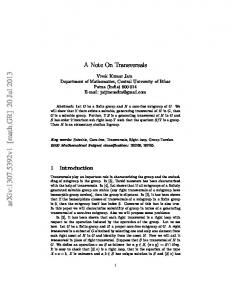
Notice that det ∇y ∈ W 1,∞ (Ω), Cof ∇y ∈ W 1,∞ (Ω; R3×3 ), (det ∇y)−1/(4t+3) ∈ L1 (Ω) but we see that ∇2 y 6∈ L1 (Ω; R3×3×3 ) which means that y 6∈ W 2,1 (Ω; R3 ). On the other hand, y ∈ W 1,p (Ω; R3 )∩ L∞ (Ω; R3 ) for every 1 ≤ p < 1 + t.

x2

x1

Figure 1: Deformed cube (green) in the frame of the reference domain (0, 1)3 as in Example 5.3 for t = 100. Therefore, the setting of gradient polyconvex materials is indeed more general than the standard approach used in non-simple materials involving the second gradient of the deformation.

19

Remark 5.4. (i) If n = 2 and F ∈ R2×2 then Cof F has the same set of entries as F (up to the minus sign at off-diagonal entries), so that J in (5.8) in fact depends on ∇2 y. (ii) If y : Ω → R3 is smooth and if ∇[Cof ∇y] = 0, almost everywhere in Ω ⊂ R3 then for almost all x ∈ Ω we have y(x) = Ax + b for some A ∈ R3×3 and b ∈ R3 , and vice versa. (iii) We recall that det ∇y and Cof ∇y measure volume and area changes, respectively, between the reference and the deformed configurations. Therefore, gradient polyconvexity ensures that these changes are not too “abrupt”. ˆ (∇y(x), ∇[Cof ∇y(x)], ∇[det ∇y(x)]) equals The principle of frame indifference requires that W ˆ (R∇y(x), ∇[Cof R∇y(x)], ∇[det R∇y(x)]) for every y : Ω → R3 as in Definition 5.1 and every W R ∈ SO(3). Since ∇[det R∇y] = ∇[det ∇y] and ∇[Cof (R∇y)] = ∇[Cof RCof ∇y] = ∇[RCof ∇y] = R∇[Cof ∇y], frame indifference translates to ˆ (F, ∆1 , ∆2 ) = W ˆ (RF, R∆1 , ∆2 ) W

(5.3)

for every F ∈ R3×3 , every ∆1 ∈ R3×3×3P , every ∆2 ∈ R3 , and every proper rotation R ∈ SO(3). We recall that componentwise [R∆1 ]ijk := 3m=1 Rim [∆1 ]mjk for all i, j, k ∈ {1, 2, 3}. Let us now turn to our existence theorems for gradient polyconvex energies. As already pointed out in Remark 5.2, we can do so, only when prescribing suitable coercivity conditions. We are ˆ does not actually going to assume, essentially, two types of growth conditions: In the first case, W depend on ∇[det ∇y], so that we assume that for some c > 0, and finite numbers p, q, r, s ≥ 1 it holds that ( p + |Cof F |q + (det F )r + (det F )−s + |∆ |q c |F | if det F > 0, 1 ˆ (F, ∆1 ) ≥ W (5.4) +∞ otherwise. Notice that even if the energy does not depend on ∇[det ∇y], we will be able to prove not only existence of minimizers but also H¨ older continuity of the Jacobian. This is due to the fact that for every invertible F ∈ Rn×n Cof F := (det F )F −> ∈ Rn×n .

(5.5)

det Cof F = (det F )n−1

(5.6)

and consequently

so that Hölder continuity of the cofactor also yields (local) Hölder√continuity for the determinant. Notice also that if F ∈ R3×3 with det F > 0 then F −> = Cof F/ det Cof F , so that Cof F fully characterizes F . Therefore, Proposition 5.1 is formulated in such a way that a locking constraint L(∇y) ≤ 0 is included. Setting L := 0 makes this condition void. ˆ depend additionally on the gradient of the Jacobian and assume In the second case, we let W that for some c > 0, and finite numbers p, q, r, s ≥ 1 it holds that ( if det F > 0, c |F |p + |Cof F |q + (det F )r + (det F )−s + |∆1 |q + |∆2 |r ˆ W (F, ∆1 , ∆2 ) ≥ (5.7) +∞ otherwise. This will allow us to broaden the parameter regime for q in Proposition 5.4 and still be able to prove existence of minimizers along with the locking constraint det F ≥ ε. 20

In the following existence theorems, we consider gradient polyconvex functionals that allow also for a linear perturbation. Assume that ` is a continuous and linear functional on deformations and that I defined in (5.1) is gradient polyconvex. Define for y : Ω → R3 smooth enough the following functional J(y) := I(y) − `(y) ,

(5.8)

where I is as in Definition 5.1. Proposition 5.1. Let Ω ⊂ R3 be a bounded Lipschitz domain, and let Γ = Γ0 ∪ Γ1 be a measurable partition of Γ = ∂Ω with H(Γ0 ) > 0. Let further ` : W 1,p (Ω; R3 ) → R be a linear bounded functional and J as in (5.8) with Z ˆ (∇y, ∇[Cof∇y])dx I(y) := W (5.9) Ω

being gradient polyconvex and such that (5.4) holds true. Let L : R3×3 → R be lower semicontinuous. p Finally, let p ≥ 2, q ≥ p−1 , r > 1, s > 0 and assume that for some given map y0 ∈ W 1,p (Ω; R3 ) the following set A : = {y ∈ W 1,p (Ω; R3 ) : Cof ∇y ∈ W 1,q (Ω; R3×3 ), det ∇y ∈ Lr (Ω), (det ∇y)−s ∈ L1 (Ω), det ∇y > 0 a.e. in Ω, L(∇y) ≤ 0 a.e. in Ω, y = y0 on Γ0 } is nonempty and that inf A J < +∞. Then the following holds: (i) The functional J has a minimizer on A, i.e., inf A J is attained. (ii) Moreover, if q > 3 and s > 6q/(q − 3) then there is ε > 0 such that for every minimizer y˜ ∈ A ¯ of J it holds that det ∇˜ y ≥ ε in Ω. Before continuing with the proof, we recall that the cofactor of an invertible matrix F ∈ R3×3 consists of all nine 2 × 2 subdeterminants of F ; cf. (5.5). If A ∈ R2×2 and |A| denotes the Frobenius norm of A, then the Hadamard inequality implies |A|2 . 2 Applying (5.10) to all nine 2 × 2 submatrices of F ∈ R3×3 we get |det A| ≤

3 |Cof F | ≤ |F |2 . 2

(5.10)

(5.11)

Since Cof F −1 =

F> = (Cof F )−1 , det F

(5.12)

we have 3 |(Cof F )−1 | ≤ |F −1 |2 . 2 3×3 It follows from (5.6) that if F ∈ R is invertible then det Cof F = det2 F = det F 2 ,

(5.13)

(5.14)

where det2 F := (det F )2 . Finally, we recall (cf. [21, Proposition 2.32], for instance) that F 7→ det F is locally Lipschitz and that there is d > 0 such that for every F1 , F2 ∈ R3×3 |det F1 − det F2 | ≤ d(1 + |F1 |2 + |F2 |2 )|F1 − F2 | . 21

(5.15)

Proof. We first prove the claim (i). Let {yk } ⊂ A be a minimizing sequence of J. We get that sup kyk kW 1,p (Ω;R3 ) + kCof ∇yk kW 1,q (Ω;R3×3 ) k∈N + kdet ∇yk kLr (Ω) + k(det ∇yk )−s kL1 (Ω) < C,

(5.16)

ˆ , (5.4), and Dirichlet boundary conditions on Γ0 . Standard for some C > 0 due to coercivity of W results on weak convergence of minors [16, Theorems 7.6-1 and 7.7-1] show that (for a non-relabeled) subsequence yk * y in W 1,p (Ω; R3 ), Cof ∇yk * Cof ∇y in Lq (Ω; R3×3 ) and det ∇yk * det ∇y in Lr (Ω) for k → +∞. By weak sequential compactness of bounded sets in W 1,q (Ω; R3×3 ) we also have that Cof ∇yk * H in W 1,q (Ω; R3×3 ) for some H ∈ W 1,q (Ω; R3×3 ). In particular, Cof ∇yk → H in Lq (Ω; R3×3 ). But this implies that H = Cof ∇y. Hence, there is a subsequence (not relabeled) such that Cof ∇yk → Cof ∇y pointwise almost everywhere in Ω for k → +∞. Formula (5.14) yields that det ∇yk → det ∇y pointwise almost everywhere in Ω for k → +∞, too. We must show that y ∈ A. Since det ∇yk > 0 almost everywhere, we have det ∇y ≥ 0 in the limit. Moreover, conditions (5.4), (5.16), and the Fatou lemma imply that Z Z 1 1 +∞ > lim inf J(yk ) + `(yk ) ≥ lim inf dx ≥ dx, s s k→+∞ k→+∞ Ω (det ∇yk (x)) Ω (det ∇y(x)) hence, inevitably, det ∇y > 0 almost everywhere in Ω and (det ∇y)−s ∈ L1 (Ω). Finally, the continuity of the trace operator shows that y ∈ A. By (5.5) we have (Cof ∇yk (x))> (∇yk (x))−1 = det ∇yk (x) and thus, for almost all x ∈ Ω (∇yk (x))−1 −→ (∇y(x))−1 .

(5.17)

Notice that, due to (5.13), for almost all x ∈ Ω 3 |∇yk (x)| = det ∇yk (x)|(Cof (∇yk (x))−> | ≤ det ∇yk (x)|(∇yk (x))−1 |2 < C(x) 2 for some C(x) > 0 independent of k ∈ N, i.e., we may select a (x-dependent) convergent subsequence of {∇yk (x)}k∈N called {∇ykm (x)}m∈N . Moreover, we have due to (5.13) for the fixed x ∈ Ω and m → +∞ ∇ykm (x) = det ∇ykm (x)(Cof (∇ykm (x))−> −→ det ∇y(x)(Cof (∇y(x))−> = ∇y(x), Now, as the limit is the same for all subsequences of {∇yk (x)}k∈N , namely ∇y(x), we get that the whole sequence converges pointwise almost everywhere. This also shows that for almost every x ∈ Ω we have L(∇y(x)) ≤ lim inf k→+∞ L(∇yk (x)) ≤ 0 because L is lower semicontinuous. Hence, y ∈ A. As the Lebesgue measure of Ω is finite, we get by the Egoroff theorem that ∇yk → ∇y in measure, see e.g. [27, Theorem 2.22]. ˆ and due to convexity of W ˆ (F, ·) we have by [27, Due to continuity and nonnegativity of W Corollary 7.9] that Z Z ˆ ˆ (∇yk (x), ∇[Cof ∇yk (x)]) dx. W (∇y(x), ∇[Cof ∇y(x)]) dx ≤ lim inf W (5.18) Ω

k→+∞

22

Ω

To pass to the limit in the functional `, we exploit its linearity. Hence, J is weakly lower semicontinuous along {yk } ⊂ A and y ∈ A is a minimizer of J. This proves (i). ¯ Let us prove (ii). If q > 3, the Sobolev embedding theorem implies that Cof ∇y ∈ C 0,α (Ω), where α = (q − 3)/q < 1. We first show that det ∇y > 0 on ∂Ω. Assume that there is x0 ∈ ∂Ω such that det ∇y(x0 ) = 0. We can, without loss of generality, assume that x0 := 0 and estimate for all ¯ x∈Ω 0 ≤ |Cof ∇y(x) − Cof ∇y(0)| ≤ C|x|α , where C > 0. Taking into account (5.14), (5.15), and the fact that Cof ∇y is uniformly bounded on Ω, we have for some K, d˜ > 0 that ˜ 0 ≤ det2 ∇y(x) = |det Cof ∇y(x) − det Cof ∇y(0)| ≤ d|Cof ∇y(x) − Cof ∇y(0)| ≤ K|x|α . (5.19) Altogether, we see that if |x| ≤ t then 1 1 ≥ . (det2 ∇y(x))s/2 K s/2 tαs/2 We have for t > 0 small enough Z Ω

1 dx ≥ (det ∇y(x))s

Z B(0,t)∩Ω

ˆ 3 1 Kt dx ≥ , (det2 ∇y(x))s/2 K s/2 tαs/2

(5.20)

ˆ 3 ≤ L3 (B(0, t) ∩ Ω) and K ˆ > 0 is independent of t for t small enough. Note that this is where Kt possible because Ω is RLipschitz and therefore it has the cone property. Passing to the limit for t → 0 in (5.20) we see that Ω (det ∇y(x))−s dx = +∞ because αs/2 = ((q − 3)/q)s/2 > 3. This, however, contradicts our assumptions and, consequently, det ∇y > 0 everywhere in ∂Ω. If we assume that there is x0 ∈ Ω such that det ∇y(x0 ) = 0 the same reasoning brings us again to a contradiction. It ¯ is compact and x 7→ det ∇y(x) is is even easier because B(x0 , t) ⊂ Ω for t > 0 small enough. As Ω ¯ This finishes the proof of (ii) continuous it is clear that there is ε > 0 such that det ∇y ≥ ε in Ω. if there is a finite number of minimizers. Assume then that there are infinitely many minimizers of J and assume that such ε > 0 does not ¯ such that exist, i.e., that for every k ∈ N there existed yk ∈ A such that J(yk ) = inf A J and xk ∈ Ω 2 det ∇yk (xk ) < 1/k. We can even assume that xk ∈ Ω because of the continuity of x 7→ det2 ∇yk (x). The uniform (in k) H¨ older continuity of x 7→ det2 ∇yk (x) which comes from (5.4) and from the fact that J(yk ) = inf A J implies that |det2 ∇yk (x) − det2 ∇yk (xk )| ≤ K|x − xk |α (with K independent of k) and therefore 0 ≤ det2 ∇yk (x) ≤ 1/k + K|x − xk |α . Take rk > 0 so small that B(xk , rk ) ⊂ Ω for all k ∈ N. Then s/2 Z Z Z k 2 −s/2 2 −s/2 inf J ≥ (det ∇yk (x)) dx ≥ (det ∇yk (x)) dx ≥ dx. α A Ω B(xk ,rk ) B(xk ,rk ) 1 + Kkrk The right-hand side is, however, arbitrarily large for k suitably large and rk suitably small because αs > 6. This contradicts inf A J < +∞. The proof of (ii) is finished.

23

Remark 5.5. A claim analogous to (ii) has already been proved by Healey and Kr¨ omer [32], who 2,p 3 showed it for deformations in W (Ω; R ) with p large enough so that the determinant is H¨ older continuous. We can ensure the latter even for gradient polyconvex materials, i.e., even though the integrability of second derivatives of the deformation is not guaranteed. Remark 5.6. (i) Using (5.14), (5.15), and [39, Thm. 1] we obtain that under the assumptions of Proposition 5.1 every y ∈ A satisfies det2 ∇y = det Cof ∇y ∈ W 1,r (Ω) where ( 3q/(9 − 2q) if 9/5 ≤ q < 3, r := q if q > 3. One cannot, however, infer any Sobolev regularity of det ∇y from this result because a 7→ locally Lipschitz on nonnegative reals; cf. [39, Thm. 1] for details.

√

a is not

(ii) Having y ∈ W 2,p (Ω; R3 ) we get from [39, Thm. 1] that Cof ∇y ∈ W 1,q (Ω; R3×3 ) where ( 3p/(6 − p) if 3/2 ≤ p < 3, q := p if p > 3. Remark 5.7. (i) The nonemptiness of A must be explicitly assumed because a precise characterization of the set of traces of Sobolev maps with positive determinant almost everywhere in Ω is not known. Thus, given a boundary datum y0 there is no more explicit way to assure that it is compatible with deformations of finite energy than the assumption that A is non-empty. We also refer to [12, Section 7] for more details on this topic. ˆ in its first component is not required in the existence (ii) Let us point out that convexity of W result in Proposition 5.1. This is, on one hand, not surprising since the energy depends (in parts) also on the second gradient. On the other hand, we know that boundedness of the second gradient may not be assured so that no compact embedding can be used to see that the minimizing sequence actually converges strongly in W 1,p (Ω; R3 ) to pass to the limit in the terms depending on ∇y(x). Actually our proof relies only on pointwise convergence that can be deduced from Cramer’s rule for the matrix inverse, cf. (5.5), so that it combines analytical and algebraic results. The technique of the proof of Proposition 5.1 can actually be used to show the following strong compactness result which might be of an independent interest. Different variants of the proposition are certainly available, too. Proposition 5.2. Let Ω ⊂ R3 , be a Lipschitz bounded domain and let {yk }k∈N ⊂ W 1,p (Ω; R3 ) for p > 3 be such that for some s > 0 sup kyk kW 1,p (Ω;R3 ) + kCof ∇yk kBV(Ω;R3×3 ) + k|det ∇yk |−s kL1 (Ω) < +∞. (5.21) k∈N

Then there is a (nonrelabeled) subsequence and y ∈ W 1,p (Ω; R3 ) such that for k → +∞ we have the following convergence results: yk → y in W 1,d (Ω; R3 ) for every 1 ≤ d < p, det ∇yk → det ∇y in Lr (Ω) for every 1 ≤ r < p/3, Cof ∇yk → Cof ∇y in Lq (Ω; R3×3 ) for every 1 ≤ q < p/2, and |det ∇yk |−t → |det ∇y|−t in L1 (Ω) for every 0 ≤ t < s. Moreover, if s > 3 then (∇yk )−1 → (∇y)−1 in Lα (Ω; R3×3 ) for every 1 ≤ α < 3s/(3s + 3 − s). 24

In the above proposition, BV(Ω; R3×3 ) stands for the space of functions of bounded variations. Proof. Reflexivity of W 1,p (Ω; R3 ) and (5.21) imply the existence of a subsequence of {yk } (which we do not relabel) such that yk * y in W 1,p (Ω; R3 ). Moreover, by the compact embedding of BV(Ω) to L1 (Ω), we extract a further subsequence satisfying Cof ∇yk → H in L1 (Ω; R3×3 ). Weak continuity of y 7→ det ∇y : W 1,p (Ω; R3 ) → Lp/3 (Ω) and of y 7→ Cof ∇y : W 1,p (Ω; R3 ) → Lp/2 (Ω; R3×3 ) [21] implies that H = Cof ∇y. The strong convergence in L1 yields that we can extract a further subsequence ensuring Cof ∇yk → Cof ∇y a.e. in Ω and in view of (5.6) also det ∇yk → det ∇y a.e. in Ω. By the Fatou lemma and the assumption (5.21) Z Z 1 1 +∞ > lim inf dx ≥ dx, s s k→+∞ Ω |det ∇yk (x)| Ω |det ∇y(x)| which shows that det ∇y 6= 0 almost everywhere in Ω. Reasoning analogously to the one in the proof of Proposition 5.1 results in the almost everywhere convergence ∇yk → ∇y for k → +∞. The Vitali convergence theorem (see e.g. [27, Theorem 2.24]) then implies that ∇yk → ∇y in Ld (Ω; R3×3 ) for every 1 ≤ d < p. This shows the strong convergence of yk → y in W 1,d (Ω; R3 ). The same argument gives the other strong convergences of the determinant and the cofactor. The standard embedding result [2] implies that supk∈N kCof ∇yk kL3/2 (Ω;R3×3 ) < +∞. As {(det ∇yk )−1 }k∈N ⊂ Ls (Ω) is uniformly bounded, too, the Hölder inequality and the Vitali convergence theorem imply the strong convergence of (∇yk )−1 → (∇y)−1 in Lα (Ω; R3×3 ). Let us finally mention that Proposition 5.1 can be easily generalized to integral functionals Z I(y) := W(x, y(x), ∇y(x), (∇y(x))−1 , ∇[Cof ∇y(x)]) dx (5.22) Ω

where W : Ω × R3 × R3×3 × R3×3 × R3×3×3 → R is such that W is a normal integrand (i.e., measurable in x ∈ Ω if the other variables are fixed and lower semicontinuous in the other variables if almost every x ∈ Ω is fixed) and W(x, yˆ, F, F −1 , ·) : R3×3×3 × R3 → [0, +∞] is convex for almost every x ∈ Ω, every yˆ ∈ R3 , and every F ∈ R3×3 . If, further, for some c > 0, s > 0, p, q, r ≥ 1, and g ∈ L1 (Ω) it holds that for almost all x ∈ Ω and all y˜ ∈ R3 , F ∈ R3×3 , and ∆1 ∈ R3×3×3 ( c |F |p + |Cof F |q + (det F )r + (det F )−s + |∆1 |q − g(x) if det F > 0, −1 W(x, yˆ, F, F , ∆1 ) ≥ +∞ otherwise (5.23) then we have the following result, which can be phrased not only for the physically most interesting case n = 3, but for arbitrary dimensions n ≥ 2. Proposition 5.3. Let Ω ⊂ R3 be a bounded Lipschitz domain, and let Γ = Γ0 ∪ Γ1 be a measurable partition of Γ = ∂Ω with H2 (Γ0 ) > 0. Let I be as in (5.22) and such that (5.23) holds true with p some g ∈ L1 (Ω). Let L : R3×3 → R be lower semicontinuous. Finally, let p ≥ 2, q ≥ p−1 , r > 1, 1,p 3 s > 0 and assume that for some given map y0 ∈ W (Ω; R ) the following set A : = {y ∈ W 1,p (Ω; R3 ) : Cof ∇y ∈ W 1,q (Ω; R3×3 ), det ∇y ∈ Lr (Ω), (det ∇y)−s ∈ L1 (Ω), det ∇y > 0 a.e. in Ω, L(∇y) ≤ 0 a.e. in Ω, y = y0 on Γ0 } 25

is nonempty and that inf A I < +∞. Then the following holds: (i) the functional I has a minimizer on A. (ii) Moreover, if q > 3 and s > 6q/(q − 3) then there is ε > 0 such that for every minimizer y˜ ∈ A ¯ of I it holds that det ∇˜ y ≥ ε in Ω. Sketch of proof. The proof follows the lines of the proof of Proposition 5.1. We can assume that a minimizing sequence {yk }k∈N ⊂ A converges in measure to y ∈ A due to the compact embedding of W 1,p (Ω; R3 ) into Lp (Ω; R3 ). Moreover, {∇yk }k∈N and {(∇yk )−1 }k∈N converge in measure, too; cf. (5.17). Then we again apply [27, Cor. 7.9] with v := ∇[Cof ∇y], u := (y, ∇y, (∇y)−1 ), f := W+g, E := Ω, and correspondingly for the sequences. ˆ depending also on the Let us now turn our attention to gradient polyconvex energies with W gradient of the Jacobian in a convex way as in (5.1). This setting allows for a stronger result with respect to the determinant constraint: Here, we only require the Sobolev index r related to the determinant to be larger than in the existence result but leave the Sobolev index q giving the regularity of the cofactor matrix the same, compare Propositions 5.1 and 5.4. Proposition 5.4. Let Ω ⊂ R3 be a bounded Lipschitz domain, and let Γ = Γ0 ∪ Γ1 be a measurable partition of Γ = ∂Ω with H(Γ0 ) > 0. Let further ` : W 1,p (Ω; R3 ) → R be a linear bounded functional and J as in (5.8) with I being gradient polyconvex and such that (5.7) holds true. Let L : R3×3 → R p be lower semicontinuous. Finally, let p ≥ 2, q ≥ p−1 , r > 1, s > 0 and assume that for some given 1,p 3 map y0 ∈ W (Ω; R ) the following set A : = {y ∈ W 1,p (Ω; R3 ) : Cof ∇y ∈ W 1,q (Ω; R3×3 ), det ∇y ∈ W 1,r (Ω), (det ∇y)−s ∈ L1 (Ω), det ∇y > 0 a.e. in Ω, L(∇y) ≤ 0 a.e. in Ω, y = y0 on Γ0 } is nonempty and that inf A J < +∞. Then the following holds: (i) The functional J has a minimizer on A. (ii) Moreover, if r > 3 and s > 3r/(r − 3) then there is ε > 0 such that for every minimizer y˜ ∈ A ¯ of J it holds that det ∇˜ y ≥ ε in Ω. Sketch of proof. We proceed exactly as in the proof of Proposition 5.1. If {yk }k∈N ⊂ A is a minimizing sequence for J we get by standard arguments [4, 16] that det ∇yk * det ∇y in Lr (Ω) for k → +∞. At the same time, we can assume that det ∇yk * δ in W 1,r (Ω) for some δ ∈ W 1,r (Ω). These two facts imply that δ = det ∇y. This shows (i). In order to prove (ii) we again argue by a ¯ such that det ∇y(x0 ) = 0. Let again x0 := 0, so that contradiction. Assume that there is x0 ∈ Ω det ∇y(0) = 0. Then we get from the Hölder estimate for almost every x ∈ Ω 0 ≤ det ∇y(x) = |det ∇y(x) − det ∇y(0)| ≤ K|x|α ,

(5.24)

where α = (r − 3)/r. Similar reasoning as in (5.20) implies the result.

Remark 5.8 (Global invertibility of deformations). A global (a.e.) invertibility condition, the socalled Ciarlet-Neˇcas condition [18], Z det ∇y(x) dx ≤ L3 (y(Ω)) (5.25) Ω

26

can be easily imposed on the minimizer if p > 3 and the proof proceeds exactly in the same way as in [18]. This means that there is ω ⊂ Ω, L3 (ω) = 0, such that y : Ω \ ω → y(Ω \ ω) is injective. As y satisfies Lusin’s N-condition, we also have that L3 (y(Ω \ ω)) = L3 (y(Ω)). If |∇y|3 /det ∇y ∈ L2+δ (Ω) for some δ > 0 and (5.25) holds then we even get invertibility everywhere in Ω due to [33, Theorem 3.4]. Namely, this then implies that y is an open map. Moreover, the 3 mapping even polyconvex and positive if F ∈ R3×3 and det F > 0, hence the R F 7→ |F3 | /det F is 2+δ term Ω (|∇y(x)| /det ∇y(x)) dx can be easily added to the energy functional and it preserves its weak lower semicontinuity, see [4, 16] for details. Open problem. Is it possible to construct y such that y ∈ A and y 6∈ W 2,1 (Ω; R3 ) if r and s ¯ ? are as in (ii) of Proposition 5.4 and det ∇y > 0 in Ω A partial negative answer can be obtained in the following case: consider Ω ⊂ R3 a bounded Lipschitz domain, F : Ω → R3×3 such that Cof F ∈ W 1,q (Ω; R3×3 ) for 3 > q ≥ 3/2, det F ≥ ε > 0 in Ω for some ε > 0, and det F ∈ W 1,r (Ω) for some r > 3. Then F ∈ W 1,3q/(6−q) (Ω; R3×3 ). Moreover, if 3 < q then F ∈ W 1,q (Ω; R3×3 ). Indeed, as det F ≥ ε we get that 1/det F = h(det F ), where h : R → (0, ∞) with ( 1/|a| if |a| ≥ ε, h(a) := 1/ε otherwise. Since h is a Lipschitz function, we get by [39, Thm. 1] that (det F )−1 ∈ W 1,r (Ω). In view of (5.5), [58, Thm. 1] and Cof F ∈ W 1,q (Ω; R3×3 ) we get that F −1 ∈ W 1,q (Ω; R3×3 ). Applying (5.5) to F −1 we get that F = det F (Cof F −1 )> whose regularity again follows from [39, Thm. 1] [58, Thm. 1]. It remains to apply the previous reasoning to F := ∇y to show that minimizers ∗ obtained in (ii) of Propositions 5.3 and 5.4 satisfy y ∈ W 2,min(p ,3q/(6−q)) (Ω; R3 ) if 3/2 ≤ q < 3 or ∗ y ∈ W 2,min(p ,q) (Ω; R3 ) if q > 3. In both cases:   if p < 3, 3p/(3 − p) ∗ p := arbitrary number ≥ 1 if p = 3,   +∞ if p > 3. In the next example we provide a modification of the well-known Saint Venant-Kirchhoff material that is gradient polyconvex. Example 5.9. Let ϕ : R3×3 → R be a stored energy density of an anisotropic Saint VenantKirchhoff material, i.e., 1 0 ≤ ϕ(F ) := C(F > F − Id) : (F> F − Id), 8 where C is the fourth-order and positive definite tensor of elastic constants, and “:” denotes the scalar product between matrices. Therefore, ϕ(F ) ≥ c(|F |4 − 1) for some c > 0 and all matrices F and ϕ(F ) = 0 if and only if F = Q for some (not necessarily proper) rotation Q. We define ( ϕ(F ) + α(|∆1 |q + (det F )−s ) if det F > 0, ˆ W (F, ∆1 ) := (5.26) +∞ otherwise ˆ is admissible for F ∈ R3×3 and ∆1 ∈ R3×3×3 , and for some α > 0, s > 0, and q = 2. Then W in Definition 5.1, and Proposition 5.1 can be readily applied with p = 4. We emphasize that ϕ is 27

widely used in engineering/computational community because it allows for an easy implementation of all elastic constants. On the other hand, ϕ is not quasiconvex which means that existence of minimizers cannot be guaranteed. Additionally, ϕ stays locally bounded even in the vicinity of nonˆ cures the invertible matrices and thus allows for non-realistic material behavior. The function W mentioned drawbacks and (5.26) offers a mechanically relevant alternative to the Saint Venantˆ does not admit any change of the orientation and W ˆ (F, ∆1 ) → +∞ if Kirchhoff model. Indeed, W det F → 0+ . Obviously, other gradient-polyconvex variants of (5.26) are possible, too. Let us remark that Propositions 5.1, 5.3 and 5.4 can be further used to get existence results for static as well as for rate-independent evolutionary problems describing shape memory materials, elasto-plasticity with non-quasiconvex energy densities, for instance, or for their mutual interactions as in [31] or [37], respectively. The main idea of the proofs remains unchanged, however. We also refer to [40] for a thorough review of mathematical results on rate-independent processes with many applications to materials science. Acknowledgment: This work was partly conducted when MK held the Giovanni-Prodi Chair in the Institute of Mathematics, University of W¨ urzburg. The invitation, hospitality, and support are gratefully acknowledged. We thank Jan Valdman for providing us with Figure 1, Nicola Fusco for mentioning his interest in the general functional (5.22), Stefan Krömer for interesting discussions, and two anonymous referees for very valuable comments. This research was also supported by the ˇ grant 17-04301S, by the DAAD–AVCR ˇ project DAAD 16-14 and PPP 57212737 with funds GACR from BMBF.

References [1] Alicandro, R., Lazzaroni, G., Palombaro, M.: On the effect of interactions beyond nearest neighbours on nonconvex lattice systems. Calc. Var. PDE 56 (2017), 42. [2] Ambrosio, L., Fusco, N., Pallara, D.: Functions of Bounded Variation and Free Discontinuity Problems. Oxford Mathematical Monographs, Oxford, The Claredon Press / Oxford University Press, 2000. [3] Balder, E.J.: A general approach to lower semicontinuity and lower closure in optimal control theory. SIAM J. Control Optim. 22 (1984), 570–598. [4] Ball, J.M.: Convexity conditions and existence theorems in nonlinear elasticity. Arch. Rational Mech. Anal. 63 (1977), 337–403. [5] Ball, J.M.: Some open problems in elasticity. In Geometry, Mechanics, and Dynamics, pp. 3–59, Springer, New York, 2002. [6] Ball, J.M., Crooks, E.C.M.: Local minimizers and planar interfaces in a phase-transition model with interfacial energy. Calc. Var. PDE 40 (2011), 501–538. [7] Ball, J.M., Currie, J.C., Olver, P.L.: Null Lagrangians, weak continuity, and variational problems of arbitrary order. J. Funct. Anal. 41 (1981), 135–174. [8] Ball, J.M., James, R.D.: Fine phase mixtures as minimizers of energy. Archive Rational. Mech. Anal. 100 (1988), 13–52. [9] Ball, J.M., Mora-Corral, C.: A variational model allowing both smooth and sharp phase boundaries in solids. Communications on Pure Appl. Anal. 8 (2009), 55–81.

28

[10] Beneˇsov´ a, B., Kampschulte, M.: Gradient Young measures generated by quasiconformal maps in the plane. SIAM J. Math. Anal. 47 (2015), 4404–4435. [11] Beneˇsov´ a, B., Kruˇz´ık, M.: Characterization of gradient Young measures generated by homeomorphisms in the plane. ESAIM Control Optim. Calc. Var. 22 (2016), 267–288. [12] Beneˇsov´ a, B., Kruˇz´ık, M.: Weak lower semicontinuity of integral functionals and applications. SIAM Review 59 (2017), 703–766. [13] Bhattacharya, K.: Microstructure of martensite. Why it forms and how it gives rise to the shape-memory effect. Oxford Univ. Press, New York, 2003. [14] Carbone, L., DeArcangelis, R.: Unbounded Functionals in the Calculus of Variations: Representation, Relaxation, and Homogenization. CRC Press, Boca Raton, 2001. [15] Champion, T., De Pascale, L.: Homogenization of Dirichlet problems with convex bounded constraints on the gradient. Zeit. Anal. ihre Anwendungen 22 (2003), 591–608. [16] Ciarlet, P.G.: Mathematical Elasticity Vol. I: Three-dimensional Elasticity, North-Holland, Amsterdam, 1988. [17] Ciarlet, P.G., Neˇcas, J.: Unilateral problems in nonlinear, three-dimensional elasticity. Arch. Rational Mech. Anal. 87 (1985), 319–338. [18] Ciarlet P.G., Neˇcas, J.: Injectivity and self-contact in nonlinear elasticity. Arch. Rational Mech. Anal. 97 (1987), 171–188. [19] Conti, S., Dolzmann, G.: On the theory of relaxation in nonlinear elasticity with constraints on the determinant. Arch. Rational Mech. Anal. 217 (2015), 413–437. [20] Conway, J.B.: A Course in Functional Analysis. 2nd ed., Springer, New York, 1997. [21] Dacorogna, B.: Direct Methods in the Calculus of Variations. 2nd ed., Springer, Berlin, 2008. [22] De Arcangelis, R., Zappale, E.: The relaxation of some classes of variational integrals with pointwise continuoustype gradient constraints. Appl. Math. Optim. 51 (2005), 251–277. [23] Dell’Isola, F., Sciarra, G., Vidoli, S.: Generalized Hooke’s law for isotropic second gradient materials. Proc. R. Soc. Lond. A 465 (2009), 2177–2196. [24] Demengel, F., Suquet, P.: On locking materials. Acta Applicandae Mathematicae 6 (1986), 185–211. [25] Duerinckx, M., Gloria, A.: Stochastic homogenization of nonconvex unbounded integral functionals with convex growth. Arch. Rational Mech. Anal. 221 (2016), 1511–1584. [26] Ekeland, I., Temam, R.: Convex Analysis and Variational Problems. SIAM Philadelphia, 1999. [27] Fonseca, I., Leoni, G.: Modern Methods in the Calculus of Variations: Lp Spaces. Springer, New York, 2007. [28] Forest, S.: Micromorphic approach for gradient elasticity, viscoplasticity, and damage. J. Engrg. Mech. 135 (2009), 117. https://doi.org/10.1061/(ASCE)0733-9399(2009)135:3(117). [29] Fosdick, R., Royer-Carfagni, G.: The constraint of local injectivity in linear elasticity theory. Proc. R. Soc. Lond. A 457 (2001), 2167–2187. [30] Golay, F., Seppecher, P.: Locking materials and the topology of optimal shapes. European Journal of Mechanics - A/Solids 20 (2001), 631–644. [31] Grandi, D., Stefanelli, U.: A phenomenological model for microstructure-dependent inelasticity in shapememory alloys Meccanica 49 (2014), 2265–2283.

29

[32] Healey, T.J., Kr¨ omer, S.: Injective weak solutions in second-gradient nonlinear elasticity. ESAIM Control Optim. Calc. Var. 15 (2009), 863–871. [33] Hencl, S., Koskela, P.: Lectures on Mappings of Finite Distortion, LNM 2096, Springer, Cham, 2014. [34] Kinderlehrer, D., Pedregal, P.: Characterization of Young measures generated by gradients. Arch. Rat. Mech. Anal. 115 (1991), 329–365. [35] Kinderlehrer, D., Pedregal, P.: Gradient Young measures generated by sequences in Sobolev spaces. J. Geom. Anal. 4 (1994), 59–90. [36] Koumatos, K., Rindler, F., Wiedemann, E.: Orientation-preserving Young measures. Q. J. Math. 67 (2016), 439–466. [37] Kruˇz´ık, M., Zimmer, J.: A model of shape memory alloys accounting for plasticity. IMA J. Appl. Math. 76 (2011), 193-216. [38] Lazzaroni, G., Palombaro, M., Schl¨ omerkemper, A.: A discrete to continuum analysis of dislocations in nanowire heterostructures. Commun. Math. Sci. 13 (2015), 1105–1133. [39] Marcus, M., Mizel, V.: Complete characterization of functions which act, via superposition, on Sobolev spaces. Trans. AMS 251 (1979), 187–218. [40] Mielke, A., Roub´ıˇcek, T.: Rate-Independent Systems: Theory and Applications. Springer, New York, 2015. [41] Mielke, A., Roub´ıˇcek, T.: Rate-independent elastoplasticity at finite strains and its numerical approximation. Math. Models Methods in Appl. Sci. 26 (2016), 2203–2236. [42] Morrey, C.B.: Multiple Integrals in the Calculus of Variations. Springer, Berlin, 1966. [43] M¨ uller, S.: Variational models for microstructure and phase transitions. Lecture Notes in Mathematics 1713, Springer Berlin, 1999 pp. 85–210. [44] M¨ uller, S.: A sharp version of Zhang’s theorem on truncating sequences of gradients. Trans. AMS 351 (1999), 4585–4597. [45] Panagiotopoulos, P.D.: Inequality Problems in Mechanics and Applications. Birkh¨ aser, Boston, 1985. [46] Pedregal, P.: Parametrized Measures and Variational Principles. Birk¨ auser, Basel, 1997. [47] Phillips, A.: The theory of locking materials. Transactions of The Society of Rheology 3 (1959), 13–26. [48] Podio-Guidugli, P.: Contact interactions, stress, and material symmetry, for nonsimple elastic materials. Theor. Appl. Mech. 28–29 (2002), 26—276. [49] Prager, W.: On ideal locking materials. Transactions of The Society of Rheology, 1, (1957), 169–175. [50] Rajagopal, K.R.: Non-linear elastic bodies exhibiting limiting small strain. Math. Mech. Solids 16 (2011), 122–139. [51] Roub´ıˇcek, T.: Relaxation in Optimization Theory and Variational Calculus. W. de Gruyter, Berlin, 1997. [52] Roub´ıˇcek, T.: Nonlinear Partial Differential Equations with Applications. 2nd ed., Birkh¨ aser, Basel, 2013. [53] Schuricht, F.: Locking constraints for elastic rods and a curvature bound for spatial curves. Calc. Var. PDE 24 (2005), 377–402. ˇ [54] Silhav´ y, M.: Phase transitions in non-simple bodies. Arch. Rational Mech. Anal. 88 (1985), 135–161. [55] Toupin, R.A.: Elastic materials with couple-stresses. Arch. Rational Mech. Anal. 11 (1962), 385–414.

30

[56] Toupin, R.A.: Theory of elasticity with couple-stress. Arch. Rational. Mech. Anal. 17 (1964), 85–112. [57] Valadier, M.: Young measures. In: Methods of Nonconvex Analysis (A.Cellina, ed.) Lecture Notes in Math. 1446, Springer, Berlin, 1990, pp. 152–188. [58] Valent, T.: A property of multiplication in Sobolev spaces. Some applications. Rend. Sem. Mat. Univ. Padova 74 (1985), 63–73. [59] Wagner, M.: Smoothness properties of the lower semicontinuous quasiconvex envelope. Zeit. Anal. u. ihre Anwendungen 29 (2010), 377–400. [60] Wagner, M.: On the lower semicontinuous quasiconvex envelope for unbounded integrands (I). ESAIM: Contr. Optim. Calc. Var. 15 (2009): 68–101. [61] Wagner, M.: Quasiconvex relaxation of multidimensional control problems with integrands f (t, ξ, v). ESAIM: Contr. Optim. Calc. Var. 17 (2011): 190–221. [62] Young, L.C.: Generalized curves and the existence of an attained absolute minimum in the calculus of variations. Comptes Rendus de la Société des Sciences et des Lettres de Varsovie, Classe III 30 (1937), 212–234. [63] Zhang, K.: A construction of quasiconvex functions with linear growth at infinity, Ann. Scuola Norm. Sup. Pisa 19 (1992), 313–326.

31

A note on locking materials and gradient polyconvexity

A note on locking materials and gradient polyconvexity

Suggest Documents

A NOTE ON THE GRADIENT PROJECTION

A note on gradient Einstein-type manifolds

A note on gradient elasticity and nonsingular crack fields

A Note on Reduced Strain Gradient Elasticity

A note on the nonlinear conjugate gradient method - LSEC

A NOTE ON THE GRADIENT PROJECTION ... - Semantic Scholar

On the relation between polyconvexity and rank-one ... - Springer Link

A Note On Transversals

A Note on Tubes

A note on equipartition

Gradient materials with internal constraints - Mathematical Sciences ...

Gradient composition sol-gel materials - CiteSeerX

Gradient composition sol-gel materials - CiteSeerX

A note on a critical problem with natural growth in the gradient

New tool materials with a structural gradient for milling ... - IMWF

On Synchronization and Phase Locking in Strongly

Beat-note locking in dual-polarization lasers submitted to frequency ...

Shape gradient and classical gradient of curvatures: driving forces on

Structure and properties of the gradient tool materials of ... - CiteSeerX

Structure and properties of the gradient tool materials of ... - CiteSeerX

1 Gradient image processing Edit materials and lighting

A NOTE ON THE INVARIANT AND FOLIATIONS

A note on spacelike and timelike compactness

A Note on Interfacing Object Warehouses and