ods [18, 15] to reduce the effect of state explosion. The best known .... else if t.colour = white then. 10 ... Figure 3 assigns one of four colours to each state:.
A Note on On-The-Fly Verification Algorithms Stefan Schwoon and Javier Esparza Institut f¨ ur Formale Methoden der Informatik, Universit¨ at Stuttgart {esparza,schwoosn}@informatik.uni-stuttgart.de Abstract. The automata-theoretic approach to verification of LTL relies on an algorithm for finding accepting cycles in the product of the system and a B¨ uchi automaton for the negation of the formula. Explicit-state model checkers typically construct the product space “on the fly” and explore the states using depthfirst search. We survey algorithms proposed for this purpose and propose two improved algorithms, one based on nested DFS, the other on strongly connected components. We compare these algorithms both theoretically and experimentally and determine cases where both algorithms can be useful.
1
Introduction
The model-checking problem for finite-state systems and linear-time temporal logic (LTL) is usually reduced to checking the emptiness of a B¨ uchi automaton, i.e. the product of the system and an automaton for the negated formula [23]. Various strategies exist for reducing the size of the automaton. For instance, symbolic model checking employs data structures to compactly represent large sets of states. This strategy combines well with breadth-first search, leading to solutions whose worst-case time is essentially O(n2 ) or O(n log n), if n is the size of the product. A survey of symbolic emptiness algorithms can be found in [8]. Explicit-state model checkers, on the other hand, construct the product automaton ‘on the fly’, i.e. while searching the automaton. Thus, the model checker may be able to find a counterexample without ever constructing the complete state space. On-the-fly verification can be combined with partial order methods [18, 15] to reduce the effect of state explosion. The best known on-the-fly algorithms use depth-first-search (DFS) strategies to explore the state space; their running time is linear in the size of the product automaton (i.e. the number of states plus the number of transitions). These algorithms can be partitioned into two classes: Nested DFS, originally proposed by Courcoubetis et al [5], conducts a first search to find and sort the accepting states. A second search, interleaved with the first, checks for cycles around accepting states. Holzmann et al’s modification of this algorithm [15] is widely regarded as the state-of-the-art algorithm for on-the-fly model checking and is used in Spin [14]. The advantage of this algorithm is its memory efficiency. On the downside, it tends to produce rather long counterexamples. Recently, Gastin et al [10] proposed two modifications to [5]: one to find counterexamples faster, and another to find the minimal counterexample. Another problem with Nested DFS is that its extension to generalised B¨ uchi automata creates significant additional effort, see Subsection 5.2. The other class can be characterised as SCC-based algorithms. Clearly, a counterexample exists if and only if there is a strongly connected component (SCC) that is reachable from the initial state and contains at least one accepting state and at least one transition. SCCs can be identified using, e.g.,
Tarjan’s algorithm [21]. Tarjan’s algorithm can easily accomodate generalised B¨ uchi automata, but uses much more memory than Nested DFS. Couvreur [6] and Geldenhuys and Valmari [11] have proposed modifications of Tarjan’s algorithm, whose common feature is that they recognize an accepting cycle as soon as all transitions on the cycle are explored. Thus, the search may explore a smaller part of the automaton and tends to produce shorter counterexamples. In this paper, we survey existing algorithms of both classes and discuss their relations to each other. This discussion leads to the following contributions: – We propose an improved Nested-DFS algorithm. The algorithm finds counterexamples with less exploration than [15] and [10] and needs less memory. – We analyse a simplified version of Couvreur’s algorithm [6] and show that it has advantages over the more recently proposed algorithm from [11]. We make several other interesting observations about this algorithm that were missed in [6]. With these, we reinforce the argument made in [11], i.e. that SCC-based algorithms are competitive with Nested DFS. – As a byproduct, we propose an algorithm for finding SCCs, which, to the best of our knowledge, has not been considered previously. This algorithm can be used to improve model checkers for CTL. – Having identified one dominating algorithm in each class, we discuss their relative advantages for specialised classes of automata. It is known that model checking can be done more efficiently for automata with certain structural properties [2]. Our observations sharpen the results from [2] and provide a guideline on which algorithms should be used in which case. – We suggest a modification to the way partial-order reduction can be combined with depth-first search. – Finally, we back up our findings by experimental results. We proceed as follows: Section 2 establishes the notation used to present the algorithms. Sections 3 and 4 discuss nested and SCC-based algorithms, respectively. Section 5 takes a closer look at the pros and cons of both classes, while Section 6 discusses the combination with partial order methods. Section 7 reports experiments on some examples, and Section 8 contains the conclusions and an open question.
2
Notation
The accepting cycle problem can be stated in many different variants. For now, we concentrate on its most basic form in order to present the algorithms in a simple and uniform manner. Thus, our problem is as follows: Let B = (S, T, A, s0 ), where T ⊆ S × S, be a B¨ uchi automaton (or just automaton) with states S and transitions T . We call s0 ∈ S the initial state, and A ⊆ S the set of accepting states. A path is a sequence of states s1 · · · sk , k ≥ 1, such that (si , si+1 ) ∈ T for all 1 ≤ i < k. Let dB denote the length of the longest path of B in which all states are different. A cycle is a path with s1 = sk ; the cycle is accepting if it contains a state from A. An accepting run (or counterexample) is a path s0 · · · sk · · · sl , l > k, where sk · · · sl forms an accepting cycle. The cycle detection problem is to determine whether a given automaton B has an accepting run.
1 2
procedure nested dfs () call dfs blue(s0 );
3 4 5 6 7 8 9 10
procedure dfs blue (s) s.blue := true; for all t ∈ post(s) do if ¬t.blue then call dfs blue(t); if s ∈ A then seed := s; call dfs red(s);
11 12 13 14 15 16 17
procedure dfs red (s) s.red := true; for all t ∈ post(s) do if ¬t.red then call dfs red(t); else if t = seed then report cycle;
Fig. 1. The Nested-DFS algorithm from [5].
Extensions of the problem, such as generalised B¨ uchi automata, production of counterexamples (as opposed to merely reporting that one exists), partialorder reduction, and exploiting additional knowledge about the automaton are discussed partly along with the algorithms, and partly in Sections 5 and 6. All algorithms presented below use depth-first-search strategies and are designed to work ‘on the fly’, i.e. B can be constructed during the search. In the presentation of all algorithms, we make the following assumptions: – – – –
3
Initially, the state s0 is known. Given a state s, we can compute the set post(s) := { t | (s, t) ∈ T }. For each state s, s ∈ A can be decided (in constant time). The statement report cycle ends the algorithm with a positive answer. When the algorithm ends normally, no accepting run is assumed to exist.
Algorithms based on Nested DFS
The Nested-DFS algorithm was proposed by Courcoubetis, Vardi, Wolper, and Yannakakis [5]. It can be said to consist of a blue and a red search procedure, both of which can visit any state at most once. It requires two bits per state, one for each of the searches. We assume that when a state is generated by post for the first time, both bits are false. The algorithm is shown in Figure 1. The first procedure, dfs blue, conducts a depth-first search from its argument state. The blue bit is set on all states encountered by the procedure. When the search from an accepting state s finishes, dfs red is invoked from s. This procedure sets the red bit on all the states it encounters and avoids visiting states twice. If dfs red finds that s can be reached from itself, an accepting run is reported. 3.1
Known improvements on Nested DFS
The Nested-DFS algorithm can be improved to find counterexamples earlier under certain circumstances. Consider the automaton shown in Figure 2 (a). To find the counterexample, the blue DFS must first reach the accepting state s 1 , and then the red DFS needs to go from s1 to s0 and back again to s1 , even though an accepting run is already completed at s0 . A modification suggested by Holzmann, Peled, and Yannakakis [15] eliminates this situation: As soon as a red DFS initiated at s finds a state t such that t is on the call stack of the blue DFS, the search can be terminated, because t is obviously guaranteed to reach s.
To check in constant time whether a state is on the call stack, one additional bit per state is used (or, alternatively, a hash table containing the stack states).
(b)
(a) s0
s1
s0
s1
Fig. 2. Two examples for improvements on the Nested-DFS algorithm.
Another improvement on Nested DFS was recently published by Gastin, Moro, and Zeitoun [10], who suggested the following additions: 1. The blue DFS can detect an accepting run if it finds an edge back to an accepting state that is currently on the call stack. Consider Figure 2 (b): In [15], both the blue and the red search need to search the whole automaton to find the accepting cycle. With the suggestion in [10], the cycle is found without entering the red search. We note that this improvement can be slightly generalized to include the case where the current search state is accepting and finds an edge back to a state on the stack. 2. States are marked black during the blue DFS if they have been found not to be part of an accepting run. Thus, the red search can ignore black states. However, the computational effort required to make states black is asymptotically as big as the effort expended in the red search: one additional visit to every successor state. Moreover, the effort is necessary for every blue state, even if the state is never going to be touched by the red search. Therefore, the use of black states is not necessarily an improvement.1 The algorithm from [10] requires three bits per state. 3.2 A new proposal We now formulate a version of Nested DFS that includes the improvements for early detection of cycles from [15, 10], but without the extra memory requirements. This is based on the observation that, out of the eight cases that could be encoded in [15] with the three bits blue, red, and stack, four can never happen: – A state with its blue and red bit false cannot have its stack bit set to true (obvious). – By induction, we show that no state can have its red bit set to true and its blue bit set to false, independently of its stack bit: When the red search is initiated, all successors of seed have appeared in the blue search. Later, if the red search encounters a blue state t with non-blue successor u, we can conclude that t has not yet terminated its blue search. Thus, t must be on the call stack, and the improvement of [15] will cause the red search to terminate before considering u. – The case where a state has both its red and stack bit set need not be considered: With the improvement from [15], the red search terminates as soon as it encounters a state with the stack bit. 1
The authors of [10] also propose an algorithm for finding a minimal counterexample, which has exponential worst-time complexity, and for which the black search can provide useful preprocessing. Since the scope of this paper is on linear-time algorithms, the minimization algorithm is not considered here.
1 2 3 4 5 6 7 8 9 10 11
procedure new dfs () call dfs blue(s0 ); procedure dfs blue (s) s.colour := cyan; for all t ∈ post(s) do if t.colour = cyan ∧ (s ∈ A ∨ t ∈ A) then report cycle; else if t.colour = white then call dfs blue(t); if s ∈ A then
12 13 14 15 16 17 18 19 20 21 22
call dfs red(s); s.colour := red ; else s.colour := blue; procedure dfs red (s) for all t ∈ post(s) do if t.colour = cyan then report cycle; else if t.colour = blue then t.colour := red ; call dfs red(t);
Fig. 3. New Nested-DFS algorithm.
The remaining four cases can be encoded with two bits. The algorithm in Figure 3 assigns one of four colours to each state: – white: We assume that states are white when they are first generated by a call to post. – cyan: A state whose blue search has not yet terminated. – blue: A state that has finished its blue search and has not yet been reached in a red search. – red: A state that has been considered in both the blue and the red search. The seed state of the red search is treated specially: It remains cyan during the red search and is made red afterwards. Thus, it matches the check at line 18, and the need for a seed variable is eliminated. Like in the other algorithms based on Nested DFS, the counterexample can be obtained from the call stack at the time when the cycle is reported.
4
Algorithms based on SCCs
The algorithms in this class are based on the notion of strongly-connected components (SCCs). Formally, an SCC is a maximal subset of states C such that for every pair s, t ∈ C there is a path from s to t and vice versa. The first state of C entered during a depth-first search is called the root of C. An SCC is called trivial if it consists of a single state, and if this single state does not have a transition to itself. An accepting run exists if and only if there exists a non-trivial SCC that contains at least one accepting state and whose states are reachable from s0 . In the following we present the main ideas behind three SCC-based algorithms. These explanations are not intended as a full proof, but should serve to explain the relationship between the algorithms. Tarjan [21] first developed an algorithm for identifying SCCs in linear time in the size of the automaton. His algorithm uses depth-first search and is based on the following concepts: Every state is annotated with a DFS number and a lowlink number. DFS numbers are assigned in the order in which states appear in the DFS; we assume that the DFS number is 0 when a state is first generated by post. The lowlink number of a state s is the lowest DFS number of a state t in the same SCC as s such that t was reachable from s via states that were not yet explored when the search reached s. Moreover, Tarjan maintains a set called
Current to which states are added when they are first detected by the DFS. A state is removed from Current when its SCC is completely explored, i.e. when the DFS of its root concludes. Current is represented twice, as a bit-array and as a stack. The following properties hold: (1) Current contains only states from partially explored SCCs whose roots are still on the call stack. Thus, every state in Current has a path to a state on the call stack (e.g., its root). (2) Therefore, if t is in Current when the DFS at state s detects a transition to t, t has a path to its root, from there to s, so both are in the same SCC. (3) Roots have the lowest DFS number within their SCC and are the only states whose DFS number equals their lowlink number. (4) A root r is the first state of its SCC to be added to Current. At the time when the DFS at r concludes, all other SCCs reachable from r have been completely explored and removed from Current. Thus, the nodes belonging to the SCC can be identified by removing nodes from the stack representation of Current until r is found. At the same time, one can check whether the SCC is non-trivial and contains an accepting state. For the purpose of finding accepting cycles, Tarjan’s algorithm has several drawbacks compared to Nested-DFS algorithms: It uses more memory per state (one bit plus two integers as opposed to two bits), and a larger stack: In Nested DFS, the stack may grow as large as dB whereas in Tarjan’s algorithm Current may at worst contain all states, even if dB is small. Moreover, Tarjan’s algorithm may need longer to find a counterexample: An SCC is not checked for acceptance until itself and all SCCs reachable from it have been completely explored. In Nested DFS, a red search may be started even before an SCC has been completely explored. Figure 4 illustrates this: Nested-DFS algorithms may find the cycle s0 s1 s0 and stop without examining the right part of the automaton provided that edge (s0 , s1 ) is explored before (s0 , s2 ); Tarjan’s algorithm is bound to explore the whole automaton regardless of the order of exploration.
s1
s0
s2
large subgraph without cycles
Fig. 4. Nested DFS may outperform Tarjan’s algorithm on this automaton.
Recent developments, however, have shown that Tarjan’s algorithm can be modified to eliminate or reduce some of these disadvantages, and that SCC-based algorithms can be competitive to Nested DFS. Two modifications are presented below. Their common feature is that they can detect a counterexample as soon as all transitions along an accepting run have been explored. In other words, their amount of exploration is minimal (i.e., minimal among all DFS algorithms that follow the search order given by post). 4.1 The Geldenhuys-Valmari algorithm The algorithm recently proposed by Geldenhuys and Valmari [11] extends Tarjan’s algorithm with the following idea: Suppose that the DFS starts exploring
an accepting state s. At this point, all states in Current (including s) have a path to s (property (1)). Moreover, the states that are in Current at this point can be distinguished from those that are added later by the fact that their lowlink number is less than or equal to the DFS number of s. Thus, to find a cycle including s, we need to find a state with such a lowlink number in the DFS starting at s. In [11], this is accomplished by making s a ‘target’ during the subsequent DFS. When a cycle is found, the search can be terminated immediately. An implementation of the algorithm is shown in Appendix A. The memory consumption of the Geldenhuys-Valmari algorithm is slightly higher than that of Tarjan’s due to the extra argument in the recursion. However, if a counterexample exists, the algorithm may find it earlier than Nested DFS. 4.2
Couvreur’s algorithm
Couvreur [6] proposed (in his own words) “a simple variation of the Tarjan algorithm” that solves the accepting cycle problem on generalised automata (see Subsection 5.2), but where acceptance conditions are associated with transitions. This algorithm has the advantage of detecting counterexamples early, as in [11]. Here, we translate and simplify the algorithm for the problem stated in Section 2 and then show that it has a number of additional benefits that were not considered in [6]. The following ideas, which improve upon Tarjan’s algorithm, are relevant for the algorithm: – The stack representation of Current is unnecessary. By property (4), when the DFS of a root r finishes, all other SCCs reachable from the root have already been removed from Current. Therefore, the SCC of r consists of all nodes that are reachable from r and still in Current. These can be found by a second DFS starting at r, using the bit-array representation of Current. – Lowlink numbers can be avoided. The purpose of lowlink numbers is to test whether a given state is a root. However, the DFS number already contains partial knowledge about the lowlink: it is greater than or equal to it. Couvreur’s algorithm maintains a stack (called Roots) of potential roots to which a state is added when it appears on the call stack. Recall property (2): When the DFS sees a transition from s to t after the DFS of t, and t is still in Current, then s and t are in the same SCC. A root has the lowest DFS number in its SCC. Thus, all states in the call stack with a DFS number greater than that of t cannot be roots and are removed from Roots. Moreover, these states are part of a cycle around s; if one of them is accepting, then a counterexample exists. Finally, a node r can now be identified as a root by checking whether r is still in Roots when its DFS finishes. At this point, r can also be removed from Roots. Figure 5 presents the algorithm. Even though we believe the transformation from the algorithm in [6] to be faithful, it uses different notation and solves a slightly different problem. Therefore, we provide a new proof in Appendix B. The issue of generating an actual counterexample was not considered in [6]. Fortunately, adding this is relatively easy: At line 18, the call stack plus the transition (s, t) provide a path from s0 via u to t. To complete the cycle, we
1 2 3 4 5 6 7 8 9 10 11
12 13 14 15 procedure remove (s): 16 if ¬s.current then return; 17 s.current := false; 18 for all t ∈ post(s) do remove(t); 19 20 procedure couv dfs(s): 21 count := count + 1; 22 s.dfsnum := count; push(Roots, s); s.current := true; 23
procedure couv () count := 0; Roots := ∅; call couv dfs(s0 );
for all t ∈ post(s) do if t.dfsnum = 0 then call couv dfs(t); else if t.current then repeat u := pop(Roots); if u ∈ A then report cycle; until u.dfsnum ≤ t.dfsnum; push(Roots, u); if top(Roots) = s then pop(Roots); call remove(s);
Fig. 5. Translation of Couvreur’s algorithm.
need a path from t to u, which can be found with a simple DFS within the nonremoved states starting at u (the current bit can be abused to avoid exploring states twice in this DFS). Alternatively, we could search for any state on the call stack of the DFS whose number is at least t.dfsnum, which may lead to slightly smaller counterexamples, but requires an additional ‘on stack’ bit for each state. 4.3 Comparison The algorithms presented in Subsections 4.1 and 4.2 report a counterexample as soon as all the transitions belonging to it have been explored. (For the full proofs, see [11] and Appendix B, resp.) Thus, they find the same counterexamples with the same amount of exploration. However, Couvreur’s algorithm has several advantages to those of both Tarjan and Geldenhuys and Valmari: – It needs just one integer per state instead of two. – Current is a superset of the call stack and contains at worst all the states ([11] mentions the use of stack space as a drawback). The Roots stack, however, is only a subset of the call stack. This eliminates one disadvantage of SCCbased algorithms when compared to Nested DFS. – Couvreur’s algorithm can be easily extended to multiple acceptance conditions. This is explained in greater detail in Subsection 5.2. It is not clear how such an extension could be done with the algorithm of [11]. Note that the first two advantages are not pointed out in [6]. It seems that this has caused Couvreur’s algorithm to remain largely unappreciated (as evidenced by the fact that [11] does not seem to be aware of [6]). On the downside, Couvreur’s algorithm may need two calls to post per state whereas the others need only one. 4.4 On identifying strongly connected components The algorithm in Figure 5 can be easily transformed into an algorithm for identifying the SCCs of the automaton. All that is required is to remove line 18 and to output the nodes as they are processed in the remove procedure. To the best of our knowledge, this algorithm is superior to previously known algorithms for identifying SCCs: The advantages over Tarjan’s algorithm [21] have already been pointed out; Gabow [9] avoids computing lowlink numbers, but
still uses the stack representation of Current. Nuutila and Soisalon-Soininen [17] reduce stack usage in special cases only, and still use lowlink numbers. Sharir’s algorithm [19] has none of these drawbacks, but requires reversed edges. Surprisingly, the issue of detecting SCCs was not considered in [6]. Compared to the algorithms that use a stack representation of Current, the new algorithm traverses edges twice, whereas the others traverse edges only once. This might be a disadvantage if the calls to post are computationally expensive. However, the algorithm remains linear in the size of B, and the memory savings can be significant (see Section 7). In the model-checking world, SCC decomposition is used in CTL for computing the semantics of the EG operator [4] or for adding fairness constraints [3]. Therefore, this algorithm can benefit explicit-state CTL model checkers.
5
Nested DFS vs SCC-based algorithms
In Sections 3 and 4 we have shown that the new Nested-DFS algorithm (Figure 3) and the modification of Couvreur’s algorithm (Figure 5) dominate the other algorithms in their class. Of these two, the nested algorithm is more memoryefficient: While the difference in stack usage, where the SCC algorithm consumes at most twice as much as the nested algorithm, is harmless, the difference in memory needed per state can be more significant: the nested algorithm needs only two bits, the SCC algorithm needs an integer. Nested DFS therefore remains the best alternative for combination with the bitstate hashing technique [13], which allows to analyse very large systems while potentially missing parts of the state space. If traditional, lossless hashing techniques are used, the picture is different: State descriptors even for small systems often include dozens of bytes, so that an extra integer becomes negligible. In addition, this small disadvantage of the SCC algorithm is offset by its earlier detection of counterexamples: the SCC algorithm always detects a counterexample as soon as all transitions on a cycle have been explored (i.e. with minimal exploration), while the nested algorithm may take arbitrarily longer. For instance, assume that in the automaton shown in Figure 6, the path from s1 back to s0 is explored before the subgraph starting at s2 . Then, the SCC algorithm reports a counterexample as soon as the cycle is closed, without visiting s2 and the states beyond. The nested search, however, needs to explore the large subgraph before the second DFS can start at s1 and detect the cycle.
s0
path of non−accepting states
s1
s2
large subgraph
Fig. 6. SCC-based algorithm outperforms Nested DFS on this automaton.
In Subsection 5.1, we examine how this advantage of the SCC-based algorithm is influenced by structural properties of the automaton. It turns out that for an important class of automata (namely weak automata), nested DFS avoids
the aforementioned disadavantage (and can in fact be replaced by a simple, non-nested DFS). 5.1
Exploiting structural properties ˇ In [2], Cern´ a and Pel´anek defined the following structural hierarchy of B¨ uchi automata (see also [16, 1]): – Any B¨ uchi automaton is an unrestricted automaton. – A B¨ uchi automaton is weak if and only if its states can be partitioned into sets Q1 , . . . , Qn such that each Qi , 1 ≤ i ≤ n is either contained in the set of accepting states or disjoint from it; moreover, if there is a transition from a state in Qi to a state in Qj then i ≤ j. – A weak automaton is terminal if and only if the partitions containing accepting states have no transitions into other partitions. The automata encountered in LTL model checking are the products of a system and a B¨ uchi automaton specifying some (un)desirable property. Clearly, if the specification automaton is weak or terminal, then so is its product with the system. Thus, the type of the product can be safely approximated by the type of the specification automaton, which is usually much smaller. Any run on an automaton eventually gets stuck in one of the partitions. Accepting runs of weak automata have the property that their cycle parts consist exclusively of accepting states. We now prove that the nested DFS algorithm (Figure 3) will discover (and report) an accepting run in procedure blue dfs as soon as all of its transitions have been explored: Assume that no counterexample has been completely explored so far, that the blue DFS is currently at state s, and that (s, t) is the last transition in the counterexample that has not been explored. We can assume that (s, t) is in the ‘cycle’ part of the counterexample (otherwise a complete reachable cycle would have been explored before, which violates the assumption). Therefore, both s and t must be accepting states. Then, the blue DFS will report a counterexample at line 8 if and only if t is cyan when (s, t) is explored. We prove that t is cyan by contradiction: Being an accepting state, t cannot be blue; if t is white, then discovering (s, t) will not close a cycle; and if t is red, then by construction t is not be part of a counterexample. A consequence of this is that the nested algorithm, when processing a weak automaton, always finds cycles in line 8 (when they exist). Thus, when examining weak automata, the algorithm of Figure 3 can be improved by disabling the red search (if an accepting state reaches line 11, it is not part of an accepting cycle, because such a cycle would have been found during the blue search). Thus, ˇ we end up with a simple, non-nested DFS. Cern´ a and Pel´anek [2] previously proposed simple DFS on weak systems because of its efficiency; we have shown that it also finds counterexamples with minimal exploration. Weak automata are important because they can represent (the negation of) many ‘popular’ properties, e.g. invariants (G p), inevitability (F p), progress (G F p), or response (G(p → F q)). In fact, [2] claims that 95% of the formulas in a well-known specification patterns database lead to weak automata, and propose a method that generates weak automata for a suitably restricted subset
of LTL formulas. Somenzi and Bloem [20] propose an algorithm for unrestricted formulas that attempts to produce automata that are ‘as weak as possible’. For terminal automata, [2] proposes to use simple reachability checks. For correctness, this requires the assumption that every state has a successor. For unrestricted automata, the new nested-DFS algorithm can be combined with the changes proposed by Edelkamp et al [7], which further exploit structural properties of the system and allow to combine the approach with guided search. 5.2 Handling Generalised B¨ uchi automata The accepting cycle problem can also be posed for generalised B¨ uchi automata, in which A is replaced by a set of acceptance sets A ⊆ 2S . Here, a cycle is accepting if it intersects all sets A ∈ A. Generalised B¨ uchi automata arise naturally during the translation of LTL into B¨ uchi automata (see, e.g., [12, 6]). Moreover, fairness constraints of the form G F p can be efficiently encoded with acceptance sets. Generalised B¨ uchi automata can be translated into (normal) B¨ uchi automata, but checking them directly may lead to more efficient procedures. The following paragraph briefly reviews the solutions proposed for this method: Let n be the number of acceptance sets in A. For nested DFS, Courcoubetis et al [5] proposed a method with at worst 2n traversals of each state. Tauriainen’s solution [22] reduces the number of traversals to n + 1. Couvreur’s algorithm [6] works directly on generalised automata; the number of traversals is at most 2, independently of n. This is accomplished by implementing the elements of Roots as tuples (state, set), where set contains the acceptance sets represented in the SCC of state; these sets are merged during pop sequences. Thus, Couvreur’s algorithm has a clear edge over nested DFS in the generalised case: It can detect accepting runs with minimal exploration and with less runtime overhead. 5.3 Summary The question of optimised algorithms for specialised classes of B¨ uchi automata has been addressed before in [2], as pointed out in Subsection 5.1. Likewise, [6] and [11] previously raised the point that SCC-based algorithms may be faster than nested DFS, but without addressing the issue of when this was the case. Our results show that these issues are related, which leads to the following picture: – For weak automata, simple DFS should be used by default: it is simpler and more memory-efficient than SCC algorithms and finds counterexamples with minimal exploration. – For unrestricted automata, an SCC-based algorithm should be used unless bit hashing is required. The memory overhead of Couvreur’s algorithm (Figure 5) is not significant, and it can find counterexamples with less exploration than nested DFS (and often shorter ones, see Section 7). If post is computationally expensive, Geldenhuys and Valmari’s algorithm may be preferable. – The improved nested DFS algorithm (Figure 3) should be used for unrestricted automata if bitstate hashing is needed. Note also that when generalised B¨ uchi automata can be used, the balance shifts in favour of Couvreur’s algorithm.
6
Compatibility with partial order reduction
DFS-based model checking may be combined with partial-order reduction to alleviate the state explosion problem. This technique tries not to explore all successors of a state, but only a subset matching certain conditions. In the practical approach of Peled [18], several candidate subsets of successors are tried until one is found that matches the conditions. Crucially, the chosen subset at a state s depends on the DFS call stack at s. For correctness, one must ensure that each call to post(s) choses the same subset. This can be done by (i) ensuring that the call stack is always the same for any given state, or (ii) remembering the chosen successor set, which costs extra memory. Holzmann et al [15] describe memory-efficient methods for (ii), which, however, constrain the kinds of candidate successor sets that can be used. We show that there is an alternative solution for both nested DFS and SCC-based algorithms that does not require to remember successor sets, and that does not constrain the candidate sets. Note first that the nested DFS algorithms do not have property (i); the call stack in the red DFS may differ from the one in the blue DFS. In [6], Couvreur claims that his algorithm satisfies property (i). However, adding counterexample generation destroys this property: a state can be entered with a different call stack during the extra DFS needed for generating a counterexample, see Subsection 4.2. In both cases, the methods from [15] can be used as a remedy. The alternative solution is a simple idea based on the following observations: The red search of the new nested algorithm (Figure 3) only explores cyan or blue states. The extra DFS in the SCC-based algorithm touches only states in the explored, but unremoved part of the automaton. Thus, if the partial-order reduction produces an unexplored successor during these searches, that successor can be discarded, because it cannot have been generated during the first search. In other words, the partial-order reduction may simply generate all successor states and then discard those that have not been explored before. As this solution does not impose constraints on candidate successor sets, it could lead to larger reductions at a (probably small) run-time price. We have not yet tried whether this leads to improvements in practice. No partial-orderrelated precautions are required when simple DFS is used for weak automata (see Section 5.1), as was already observed in [2].
7
Experiments
For experimental comparisons, we replicated two of the three variants from Geldenhuys and Valmari’s example [11], a leader election protocol with extinction for arbitrary networks. In both variants, the election starts over after completion; in Variant 1, the same node wins every time, in Variant 2, each node gets a turn at becoming the leader. Like in [11], the network specified in the model consisted of three nodes. Both variants were modelled in Promela. Spin [14] was used to generate the complete product state space (with partial-order reduction), and the result was given as input to our own implementation of the algorithms. All related files are at http://www.fmi.uni-stuttgart.de/szs/people/schwoon/dfs.tar.gz.
The results are summarized in Table 1. The first two sections of the table contain the results for the instances in which accepting cycles were found (for nested and SCC-based algorithms, resp.), whereas the third section contains the examples that did not contain accepting cycles. In all tables, φ indicates the LTL properties that were checked; these are again the same as in [11]. The ‘weak’ column indicates whether the resulting automaton was weak or not, ‘states’ is the total number of states in the product, and ‘trans’ the total number of transitions. (Note that the exact numbers differ from [11] because we used our own models of the algorithms). The algorithms that were compared were: – – – – –
HPY: the algorithm of Holzmann et al [15]; GMZ: the algorithm of Gastin et al [10]; New: the new nested algorithm from Figure 3; Couv: the simplified version of Couvreur’s algorithm [6], see Figure 5; GV: the algorithm of Geldenhuys and Valmari [11].
To ensure comparable results, the order of successors given by post was the same in all algorithms and was always followed. The following (implementationindependent) statistics are provided: Columns marked ‘st’ indicate the number of distinct states visited during the search; ‘tr’ indicates how many transitions were generated by calls to post, i.e. individual transitions may count more than once. ‘dp’ indicates the maximal depth of the call stack. The length of counterexamples was almost always equal to the value of ‘dp’, and only slightly less otherwise. For the SCC-based algorithms, we also provide the maximal size of their explicit state stacks. In the last section, the whole graph is explored, therefore the only differences are in the transition count, and the size of the explicit state stacks. Even though these are just a few examples, they suffice to demonstrate the most important observations made in the theoretical discussion of the algorithms. In particular, we can see the following: – The new nested-DFS algorithm finds counterexamples faster than the other nested algorithms in three cases. In those cases, the counterexamples are found as fast as in the SCC algorithms, but that is just a lucky coincidence. – The GMZ algorithm was never faster than the new algorithm, i.e. its extra black search did not provide an advantage. – The SCC-based algorithms found counterexamples earlier than HPY and GMZ on all weak automata, and earlier than the new nested algorithm in three cases. In all cases, earlier detection of counterexamples also translated to shorter counterexamples, but this is not guaranteed in general. – The Roots stack of Couvreur’s algorithm is often much smaller than the Current stack of the GV algorithm; in return, it may touch transitions twice.
8
Conclusions
We have portrayed and compared a number of algorithms for finding accepting cycles in B¨ uchi automata. A new nested-DFS algorithm was proposed, which was experimentally shown to perform better than existing ones. Moreover, we have presented an adaptation of Couvreur’s SCC-based algorithm and shown that it has important advantages, some of which were not previously observed. Thus,
Ex. w/ cycles (nested) φ weak states B E H I
no yes no no
A B E G H
no 42564 no 49256 yes 14115 yes 28126 no 111094
HPY
trans
16685 31405 4849 6081 29564 46059 29564 46059 77358 93765 17794 37457 181559
st
tr
GMZ dp
385 409 386 129 130 130 17658 21769 582 17658 21769 582 7218 16485 740 721 746 722 367 368 368 3982 4589 1040 33128 53575 906
Ex. w/ cycles (SCC) φ weak
states
trans
B E H I
no yes no no
16685 4849 29564 29564
31405 6081 46059 46059
A B E G H
no no yes yes no
42564 77358 49256 93765 14115 17794 28126 37457 111094 181559
Ex. w/o cycles
st
dp
215 130 328 328
5786 557 439 440 367 368 3982 1040 15259 798
tr
states
depth
HPY
GMZ
A C D F G
13057 3925 8964 8964 4849
312 113 312 312 312
30554 9372 20822 20822 6081
41600 9372 31868 31868 12162
C D F I
3925 27323 27323 83658
113 825 825 900
9372 66522 64512 173557
9372 100724 96704 247748
New Variant 1 30554 9372 20822 20822 6081 Variant 2 9372 66522 64512 173557
dp
214 215 215 129 129 130 17658 21769 582 17658 21769 582
740 708 368 1040 906
5786 13398 557 439 440 440 367 367 368 3982 4588 1040 33128 53575 906 GV
|Roots|
Variant 1 215 129 38249 38249 Variant 2 13398 440 367 4588 36791
tr
372 130 582 582
tr
|Current|
129 129 129 129
215 129 20009 20009
214 129 4825 4825
367 354 367 379 367
6983 440 367 4588 18998
561 439 367 3982 14091
Couv
GV
|Roots|
|Current|
41600 9372 31868 31868 12162
20800 4686 15394 15394 6081
129 113 129 129 129
4825 113 4825 4825 4825
9372 100724 96704 247748
4686 50362 48352 123874
113 367 367 367
113 14091 14091 14091
transitions explored
φ
st
Couv
dp
214 129 16132 16132
tr
Variant 1 371 392 129 129 17658 42916 17658 42916 Variant 2 7218 16498 707 729 367 367 3982 8130 33128 106364
Couv/GV st
New
stack size
Table 1. Experimental results on leader election example.
we believe that both nested DFS and SCC algorithms have their place in LTL verification; the one uses less memory, the other finds counterexamples faster. Moreover, we provide a refined judgement that takes into account structural properties of the B¨ uchi automaton. There remains an interesting open question: Is there a linear-time algorithm that combines the advantages of nested DFS and SCC-based algorithms, i.e. one
that finds counterexamples with minimal exploration and uses only a constant number of bits per state?
References 1. R. Bloem, K. Ravi, and F. Somenzi. Efficient decision procedures for model checking of linear time logic properties. In CAV’99, LNCS 1633, pages 222–235, 1999. ˇ 2. I. Cern´ a and R. Pel´ anek. Relating hierarchy of linear temporal properties to model checking. In Proc. of MFCS, LNCS 2747, pages 318–327, 2003. 3. E. Clarke, A. Emerson, and P. Sistla. Automatic verification of finite-state concurrent systems using temporal logic specifications. TOPLAS, 8:244–263, 1986. 4. E. M. Clarke, O. Grumberg, and D. A. Peled. Model Checking. MIT Press, 1999. 5. C. Courcoubetis, M. Y. Vardi, P. Wolper, and M. Yannakakis. Memory-efficient algorithms for the verification of temporal properties. Formal Methods in System Design, 1(2/3):275–288, 1992. 6. J.-M. Couvreur. On-the-fly verification of linear temporal logic. In Proc. Formal Methods, LNCS 1708, pages 253–271, 1999. 7. S. Edelkamp, A. Lluch-Lafuente, and S. Leue. Directed explicit-state model checking in the validation of communication protocols. STTT, 2004. 8. K. Fisler, R. Fraer, G. Kamhi, M. Y. Vardi, and Z. Yang. Is there a best symbolic cycle-detection algorithm? In Proc. of TACAS, LNCS 2031, pages 420–434, 2001. 9. H. N. Gabow. Path-based depth-first search for strong and biconnected components. Information Processing Letters, 74(3–4):107–114, 2000. 10. P. Gastin, P. Moro, and M. Zeitoun. Minimization of counterexamples in SPIN. In Proc. 11th SPIN Workshop, LNCS 2989, pages 92–108, 2004. 11. J. Geldenhuys and A. Valmari. Tarjan’s algorithm makes on-the-fly LTL verification more efficient. In Proc. of TACAS, LNCS 2988, pages 205–219, 2004. 12. R. Gerth, D. A. Peled, M. Y. Vardi, and P. Wolper. Simple on-the-fly automatic verification of linear temporal logic. In Proc. of PSTV, pages 3–18. IFIP, 1996. 13. G. J. Holzmann. An analysis of bitstate hashing. Formal Methods in System Design, 13(3):289–307, 1998. 14. G. J. Holzmann. The Spin Model Checker: Primer and Reference Manual. AddisonWesley, 2003. 15. G. J. Holzmann, D. A. Peled, and M. Yannakakis. On nested depth first search. In Proc. 2nd SPIN Workshop, pages 23–32, 1996. 16. O. Kupferman and M. Y. Vardi. Freedom, weakness, and determinism: From linear-time to branching-time. In Proc. of LICS, pages 81–92. IEEE, 1998. 17. E. Nuutila and E. Soisalon-Soininen. On finding the strongly connected components in a directed graph. Information Processing Letters, 49:9–14, 1994. 18. D. A. Peled. Combining partial order reductions with on-the-fly model-checking. Formal Methods in System Design, 8(1):39–64, January 1996. 19. M. Sharir. A strong-connectivity algorithm and its applications in data flow analysis. Computers and Mathematics with Applications, 7(1):67–72, 1981. 20. F. Somenzi and R. Bloem. Efficient B¨ uchi automata from LTL formulae. In Proc. of CAV, LNCS 1855, pages 248–263, 2000. 21. R. Tarjan. Depth-first search and linear graph algorithms. SIAM Journal on Computing, 1(2):146–160, 1972. 22. H. Tauriainen. Nested emptiness search for generalized B¨ uchi automata. Technical Report A79, Helsinki University of Technology, July 2003. 23. M. Y. Vardi and P. Wolper. Automata theoretic techniques for modal logics of programs. Journal of Computer and System Sciences, 32:183–221, 1986.
Appendix For convenience, this appendix provides additional information on some of the algorithms. This material is not intended for publication in the proceedings.
Appendix A Figure 7 shows a representation of the Geldenhuys-Valmari algorithm [11]. The bottom symbol (⊥) indicates that no accepting state has appeared on the call stack so far. Notice that this presentation differs from the one in [11] inasmuch as the latter is iterative instead of recursive and uses slightly different data structures. However, the differences are minor, and the presentation in Figure 7 is better suited for comparison with other algorithms. 1 2 3 4 5 6 7 8 9 10 11 12 13 14 15 16 17 18 19 20 21 22
procedure gv () count := 0; current := ∅; if s0 ∈ A then call gv dfs(s0 , s0 ); else call gv dfs(s0 , ⊥); procedure gv dfs (s, goal ) count := count + 1; s.dfsnum := count; s.lowlink := count; push(Current, s); s.current := true; for all t ∈ post(s) do if t.dfsnum = 0 then if t ∈ A then call gv dfs(t, t) else call gv dfs(t, goal ); if t.current then s.lowlink := min{s.lowlink , t.lowlink }; if goal 6= ⊥ ∧ s.lowlink ≤ goal .dfsnum then report cycle; if s.lowlink = s.dfsnum then repeat t := pop(Current); t.current := false; until s = t; Fig. 7. The Geldenhuys-Valmari algorithm.
Appendix B This appendix contains a proof of the adaptation of Couvreur’s algorithm. The proof follows the ideas from [6], but is adapted to the presentation in Figure 5 and provides more detailed explanations. We distinguish two specific parts of the automaton: – The explored part: This is the subgraph consisting of the states and the transitions that have been considered in the for-loop at line 12. – The removed part: This is the subgraph induced by the states on which the remove procedure has been called. To show that the algorithm is correct, we prove that the following three properties are invariant at line 12:
(1) Roots contains a subsequence of the call stack of the couv dfs procedure. (2) The removed part contains exactly the non-accepting SCCs of the explored part that cannot reach any of the states on the call stack. (3) All states in Roots are roots of non-accepting SCCs of the explored part. If Stack = s0 s1 . . . sn , then the SCC containing si consists of the unremoved states with numbers between si .dfsnum and si+1 .dfsnum − 1, for 0 ≤ i < n, and the SCC containing sn consists of the unremoved states with numbers greater than or equal to sn .dfsnum. It is straightforward to see that all three properties hold when line 12 is first reached in the call to couv dfs(s0 ). When a transition from s to t is considered, we distinguish the following cases: – Either t is a fresh state. In that case, t forms a new (trivial) SCC in the explored part. The procedure is now called recursively on t and t is pushed onto the stack before line 12 is reached next (in the call on t), and thus properties (1)–(3) are re-established. – Or t is in the removed part, i.e. t.in current is false in line 15. Then, due to property (2), t belongs to a non-accepting SCC and cannot reach s. Therefore, neither t nor any of its descendants can be part of an accepting cycle, and t can be ignored for the rest of the search. – Or t has been explored but not yet removed. Let r be the highest-numbered state in Roots such that r.num ≤ t.num. Then, due to property (3), r and t are in the same SCC, i.e. r can be reached from t. Because of property (1), r can reach s. Thus, we have found a cycle, and all unremoved states between r.num and count form an SCC. To re-establish property (3), we must remove all states up to, but not including, r from Roots. This is done between lines 16 and 20. Doing so preserves property (1). Due to property (3), all previous SCCs were non-accepting. Therefore, the newly agglomerated SCC is accepting if and only if one of the previous SCCs was trivial, consisting of a single accepting state. Thus the new, agglomerated SCC is accepting if and only if one of the previous roots was accepting. This condition is tested in line 18. Finally, we need to consider the actions taken when all the outgoing transitions from s have been exhausted. Because of property (1), s is either at the top of Roots or not contained in Roots at all. In the first case, s is part of an SCC whose root is higher up on the call stack, and no action needs to be taken to preserve properties (1)–(3). Otherwise, due to property (3), s is the root of a non-accepting SCC of the explored part. We need to show that s is in fact a root of the whole automaton, i.e. no states other than those mentioned in property (3) can belong to the same DFS as s: – No currently unexplored state can belong to the same DFS because all descendants of s have been explored, – No unremoved state with a lower DFS number than s can belong to the same DFS because no descendant of s could reach them (otherwise s would have been removed from Roots earlier). – No removed state can be in the same DFS because of property (2).
Thus, s is removed Roots to preserve (1) and (3). All states reachable from s have been explored, i.e. all states explored by the algorithm in the future are not reachable from s. Thus, to preserve property (2), the SCC containing s needs to be removed, which is done in line 4.2. We conclude that the algorithm is correct and detects a counterexample as soon as all of its transitions are explored because properties (2) and (3) are maintained after each processed transition: The algorithm continues only if the explored part consists exclusively of non-accepting SCCs.