where Ï(x) is the digamma function, i.e. the logarithmic derivative of the gamma function. .... Let us recall some trigonometric formulas: we have cos (arctan(x)) =.
A note on simple approximations of Gaussian type integrals with applications Christophe Chesneaua , Fabien Navarrob a LMNO,
University of Caen, France ENSAI, France
b CREST,
Abstract In this note, we introduce new simple approximations for Gaussian type integrals. A key ingredient 2 is the approximation of the function e−x by sum of three simple polynomial-exponential functions. Five special Gaussian type integrals are then considered as applications. Approximation of the Voigt error function is investigated. Keywords: Exponential approximation, Gauss integral type function, Voigt error function.
1. Motivation Gaussian type integrals play a central role in various branches of mathematics (probability theory, statistics, theory of errors . . . ) and physics (heat and mass transfer, atmospheric science. . . ). The most Ry 2 famous example of this class of integrals is the Gauss error function defined by erf(y) = √2π 0 e−x dx. As for the erf(y), plethora of useful Gaussian type integral have no analytical expression. For this reason, a lot of an approximations have been developed, more or less complicated, with more or less precision (for the erf(y) function, see [4] and the references therein). In this paper, we aim to provide acceptable and simple approximations for possible sophisticated Gaussian type integrals. We follow the simple approach of [1] which consists in expressing the 2 function e−x as a finite sum of N functions having a more tractable polynomial-exponential form: N P 2 αn |x|n e−βn |x| , where αn and βn are real numbers and n ∈ {0, . . . , N }, i.e. e−x ≈ αn |x|n e−βn |x| . n=0 2
The challenge is to chose α0 , . . . , αN and β0 , . . . , βN such that the rest function �(x) = e−x − N P αn |x|n e−βn |x| is supposed to be small: |�(x)| −1, µ ≥ 0 and p ≥ 0. We consider the following coefficients: √ α1,p = 4θ p,
α0,p = 1,
α2,p = 4θ2 p,
√ β0,p = 4θ p, 2
in such a way that our previous approximation gives: e−px ≈
√ β1,p = 3θ p, N P
√ β2,p = 2θ p,
αn,p |x|n e−βn,p |x| . Then we have
n=0
the following approximations, provided chosen ν, µ and p such that they exist: Integral approximation I. Using our approximation and [3, Case 3, Subsection 5.3], we have Z
+∞
ν −µx −px2
x e
e
dx ≈
0
2 X
αn,p
n=0
Γ(n + ν + 1) . (βn,p + µ)n+ν+1
Integral approximation II. Using our approximation and [3, Case 7, Subsection 5.5], we have +∞
Z
2
xν ln(x)e−px dx ≈
0
2 X n=0
αn,p
Γ(n + ν + 1) [ψ(n + ν + 1) − ln(βn,p )] , (βn,p )n+ν+1
where ψ(x) is the digamma function, i.e. the logarithmic derivative of the gamma function. Integral approximation III. Using our approximation and [3, Case 12, Subsection 5.3], we have Z
+∞
2 ν −µ x −px
x e
e
dx ≈
0
2 X
� αn,p 2
n=0
µ βn,p
�(ν+n+1)/2 Kn+ν+1 (2
p
µβn,p ),
where Ka (x) is the modified Bessel function of the second kind with parameter a. Integral approximation IV. Using our approximation and [3, Case 7, Subsection 7.3], we have +∞
Z
2
xν cos(υx)e−µx e−px dx ≈
0 2 X
� � � �−(n+ν+1)/2 αn,p Γ(n + ν + 1) (βn,p + µ)2 + υ 2 cos (ν + n + 1) arctan
n=0
υ βn,p + µ
�� . (2)
Let us remark that if we take υ = 0, we rediscover Integral approximation I. Integral approximation V. Using our approximation and [3, Case 8, Subsection 8.3], we have Z
+∞
2
xν sin(υx)e−µx e−px dx ≈
0 2 X
� � � � 2 2 −(n+ν+1)/2 αn,p Γ(n + ν + 1) (βn,p + µ) + υ sin (ν + n + 1) arctan
n=0
υ βn,p + µ
�� . (3)
These approximations can be useful in many domains of applied mathematics. In the next section, we illustrate the approximations (2) and (3) by investigate approximation of the Voigt error function, also 2 considered in [1] for comparison. Note that given the approximation of e−x , one can also compute Fresnel integrals, and similar related functions as well, such as other complex error functions.
3
3. Application to the Voigt error function The Voigt error function can be defined as w(x, y) = K(x, y) + iL(x, y) where Z ∞ Z ∞ t2 t2 1 1 K(x, y) = √ e− 4 e−yt cos(xt)dt, L(x, y) = √ e− 4 e−yt sin(xt)dt. π 0 π 0 Clearly, K(x, y) and L(x, y) belongs to the family of Gaussian type integrals. Further details on the Voigt error function and its numerous applications are given in [5] and [1]. It follows from the approximation (2) with the notations : p = 41 , µ = y and υ = x, that � �� � � � 1 1 � x 2 2 −2 K(x, y) ≈ √ (y + 2θ) + x cos arctan y + 2θ π !−1 � � �� � �2 x 3 + 2θ cos 2 arctan y + θ + x2 2 y + 32 θ � � �� � � 3 x 2 2 2 −2 + 2θ (y + θ) + x cos 3 arctan y+θ and, by the approximation (3), we have the same expression for L(x, y) but with sin instead of cos : � � �� � �− 1 x 1 � L(x, y) ≈ √ (y + 2θ)2 + x2 2 sin arctan y + 2θ π !−1 � �2 � � �� 3 x 2 + 2θ y+ θ +x sin 2 arctan 2 y + 23 θ � � �� � �− 3 x + 2θ2 (y + θ)2 + x2 2 sin 3 arctan . y+θ Let us recall some trigonometric formulas: we have cos (arctan(x)) = cos (3 arctan(x)) = 2
x(3−x ) 3
(1+x2 ) 2
1−3x2 3
(1+x2 ) 2
, sin (arctan(x)) =
√ x , 1+x2
√ 1 , 1+x2
sin (2 arctan(x)) =
cos (2 arctan(x)) = 2x 1+x2 ,
1−x2 1+x2 ,
sin (3 arctan(x)) =
. Using these formulas in the previous approximations of K(x, y) and L(x, y), we obtain :
� � (y + 32 θ)2 − x2 1 y + 2θ (y + θ)2 − 3x2 2 √ K(x, y) ≈ + 2θ � �2 + 2θ (y + θ) 3 �2 π (y + 2θ)2 + x2 ((y + θ)2 + x2 ) y + 32 θ + x2 and � � � 1 x 3 L(x, y) ≈ √ + 4θ y + θ � 2 π (y + 2θ)2 + x2
� 2 2 x 2 x(3(y + θ) − x ) �2 + 2θ 3 . �2 ((y + θ)2 + x2 ) y + 32 θ + x2
Let us denote by Kapp2 (x, y) and Lapp2 (x, y) the approximation above for K(x, y) and L(x, y) respectively. On the other side, we denote by Kapp1 (x, y) and Lapp1 (x, y) the approximation for K(x, y) and L(x, y) respectively proposed by [1]. The errors of the obtained approximations can be evaluated using the absolute differences for the real and imaginary parts of the complex error function defined by ∆Re∗ = |Kapp∗ (x, y) − K(x, y)|, ∆Im∗ = |Lapp∗ (x, y) − L(x, y)|. As references for K(x, y) and L(x, y) functions we used [2] which provide highly accurate results. In order to have a visual overview of the behaviour of these error functions, the curves of ∆Re∗ and ∆Im∗ are given in Figure 2. For both approximation error functions, the maximal discrepancy is observed at y = 0, more precisely, we have: max(∆Re1 ) ≈ 0.0337, max(∆Im1 ) ≈ 0.0349 and max(∆Re2 ) ≈ 0.0168, max(∆Im2 ) ≈ 0.0138. Therefore, the approximation we propose is about twice as accurate as the one proposed in [1] while maintaining its simplicity and computational advantages. 4
10 -3
0.03
15
0.02
10
0.01
5
4
4
5 2
5 2
0 0
-5
0 0
-5
10 -3
0.03
12 10 8 6 4 2
0.02 0.01
4
4
5 2 0
5 2
0 -5
0 0
-5
Figure 2: Graphical comparison of ∆Re∗ and ∆Im∗ .
[1] Abrarov, S. M. and Quine, B. M. (2018). A simple pseudo-Voigt/complex error function, arXiv:1807.09426v1. [2] Johnson, S. G. (2012). Faddeeva Package, available from http://ab-initio.mit.edu/wiki/ index.php/Faddeeva_Package. [3] Polyanin, A. and Manzhirov, A. (2008). Handbook of Integral Equations. Chapman and Hall/CRC. [4] Soranzo, A. and Epure, E. (2014). Very simply explicitly invertible approximations of normal cumulative and normal quantile function, Applied Mathematical Sciences, 8(87), 4323-4341. [5] Srivastava, H.M. and Miller, E.A. (1987). A unified presentations of the Voigt functions, Astrophys. Space Sci., 135, 111-118.
5