A Novel Algorithm for Automatic Brain Structure Segmentation from MRI Qing He, Kevin Karsch, and Ye Duan Department of Computer Science, University of Missouri-Columbia, Columbia, MO, USA, 65211 {qhgb2,krkq35}@mizzou.edu,
[email protected]
Abstract. This paper proposes an automatic segmentation algorithm that combines clustering and deformable models. First, a k-means clustering is performed based on the image intensity. A hierarchical recognition scheme is then used to recognize the structure to be segmented, and an initial seed is constructed from the recognized region. The seed is then evolved under certain deformable model mechanism. The automatic recognition is based on fuzzy logic techniques. We apply our algorithm for the segmentation of the corpus callosum and the thalamus from brain MRI images. Depending on the specific features of the segmented structures, the most suitable recognition schemes and deformable models are employed. The whole procedure is automatic and the results show that this framework is fast and robust. Keywords: Segmentation, deformable models, clustering, corpus callosum, thalamus.
1 Introduction Medical image segmentation has become crucial to the practice of medicine, but accurate, fully automatic segmentation of medical images continues to be an open problem. Two types of segmentation algorithms have appeared in previous research. One is region-based approach such as clustering, which assigns membership to pixels according to homogeneity statistics. Since there is no easier way to distinguish boundaries and interior pixels of the object, this method can lead to noisy boundaries and holes in the interior. The other class of methods is boundary-based technique such as snakes [1]. It attempts to align an initial deformable boundary with the object boundary by minimizing an energy functional which quantifies the gradient features near the boundary. The main drawback of these methods is their sensitivity to the initial conditions. To avoid being trapped in local minima, most of these algorithms require the model to be initialized near the solution or supervised by high-level guidance, which makes the automation of these methods difficult. Many model based segmentation methods have attempted to make use of substantial prior knowledge of the anatomical structures, such as shape, orientation, symmetry, and relationship to neighboring structures. Several examples can be found in [2-4]. Most of these methods however requires significantly user interaction to incorporate prior knowledge into deformable models. Recently McInerney et al. [5] G. Bebis et al. (Eds.): ISVC 2008, Part I, LNCS 5358, pp. 552–561, 2008. © Springer-Verlag Berlin Heidelberg 2008
A Novel Algorithm for Automatic Brain Structure Segmentation from MRI
553
proposed a impressive deformable organism for medical image analysis that combined deformable models and the concepts in artificial life. These organisms are endowed with intelligent sensors and aware of their behaviors during the segmentation process. A subgroup of boundary-based methods is based on active shape models [6] and active appearance models [7], which incorporate prior information to constrain shape and image appearance by learning their statistical variations. These methods are automatic, but as pointed out in [5], the effectiveness of model constraints is still dependent on appropriate initialization, and the models may latch onto nearby spurious features. Some examples can be found in [8, 9]. Several approaches [10-15] have integrated region-based and boundary-based techniques into one framework which can offer greater robustness than each technique alone. Among them, Jones and Metaxas [14] proposed a hybrid approach based on fuzzy affinity clustering. Object boundaries are estimated based on fuzzy affinity metric of multiple image features. These estimations are recursively used to guide the deformable models and updated by the new model fit. They later [15] extended the work in [14] by an automatic initialization for multiple objects. In this paper, we propose an automatic algorithm for segmenting brain structures such as the corpus callosum (CC) and the thalamus from MRI based on the integration of deformable models with region-based clustering. Our algorithm is inspired by [14,15] and follows the same spirit. However the detailed implementation is significantly different. For example, our clustering and deformable models are two sequential procedures, while they perform region-based estimation and deformable models recursively. Although we all used concepts from fuzzy logic, we use it for the purpose of recognition while they used it for affinity clustering. Our seed initialization and deformable models are also different from [14, 15]. Our framework can be summarized as follows. 1. 2. 3.
A k-means clustering is performed based on the image intensity. A hierarchical recognition scheme is used to recognize the structure to be segmented, and an initial seed is constructed from the recognized region. The seed is evolved under certain deformable model mechanism.
2 Integration of Deformable Models and Clustering We perform a k-means clustering using the following distance metric:
D =|| I ( x1 , y1 ) − I ( x 2 , y 2 ) ||
(1)
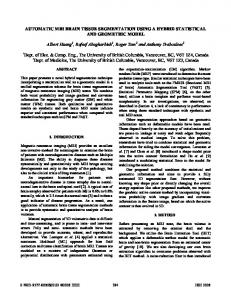
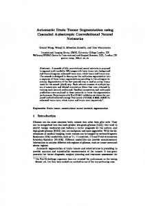
where I is the image intensity function. Pixel locations can also be used in the distance metric together with intensity, but intensity alone seems good enough for our purpose. Other clustering methods can also be used and we choose k-means because it is simple. We use eight clusters for all the CC images and two clusters for thalamus images because it fits our recognition algorithms as well as the object’s grayscale. A series of recognition schemes are then performed to recognize the interested objects from the clustering results. This results in an initial seed region whose boundary is very close to the object to be segmented. Fig. 1 and Fig. 2 show the segmentation procedures of the CC and the thalamus. More details will be discussed later.
554
Q. He, K. Karsch, and Y. Duan
(a)
(b)
(c)
(d)
Fig. 1. (a) part of an original image (b) recognition result (c) initial seed (d) final contour
(a)
(b)
(c)
(d)
Fig. 2. (a) ~ (d) are defined the same as in Fig. 1
Different deformable models are used for CC and thalamus. The boundary of the CC on the sagittal MR image is well defined by the gradient, but the existence of the fornix often makes a single active contour fail because it is almost the same brightness as the CC. We develop a fornix detection scheme in the next section which requires explicit representation of the boundary contour, thus the snake is used for deformation. The explicit contour C(p,t) evolves according to the following partial differential equation [24]:
r ∂ C ( p , t ) / ∂ t = F n , C ( p ,0 ) = C 0 ( p )
(2)
r
where n is the unit normal vector of C(p,t), F is the speed function, and t can be considered as the time parameter. The speed function is defined as:
r F = (v + εk ) g − γ (∇g • n )
(3)
where k is the curvature, v is a constant, ε , γ are coefficients, and g is a decreasing function of the image gradient. Since the seed contour is very close to the boundary and free of fornix, a simple snake can guide it to the boundary very well. The parameters in (3) need to be carefully selected in order to obtain the best performance of snakes. However, we find that one set of parameters can work for all MRI data acquired under the same condition. In our experiment, v =2, ε =0.2 and γ =0.1. On the contrary, the thalamus on the axial view usually has a simple oval shape, but the boundary is often blurred. We employ a simplified version of the level set equation in [23], which is a variation of the Mumford-Shah functional.
∂φ / ∂t = μ∇(∇φ / | ∇φ |) − λ1 (u 0 − c1 ) 2 + λ 2 (u 0 − c 2 ) 2
φ is the level set function, ∇(∇φ / | ∇φ |)
(4)
u0 is the original image, c1 and c2 are the mean intensities of the two regions, and μ , λ1 , λ 2 are is the mean curvature,
A Novel Algorithm for Automatic Brain Structure Segmentation from MRI
555
parameters. This formula allows the level set to converge using the pixel intensity inside and outside of the level set instead of gradient, which is well suited for the case of the thalamus boundary. Similar to the snakes, the local minima of level set can also be avoided because of the close-to-boundary initialization, and one set of parameter values can serve well for data with the same type. We set μ = 0.5, λ1 = 1, λ2 = 1 in our experiment.
3 Automatic Model Initialization In order to find the initial region for the deformable models from the clustering results, we design a hierarchical recognition scheme which searches the interested object from coarse level to fine level, and then an initial seed for the deformable model is generated from the recognition results. Since CC and thalamus are quite different in intensity and shape features, direct and indirect schemes are designed to recognize CC and thalamus respectively, but they both follow the same pipeline. 3.1 Coarse-Level Recognition In the coarse-level recognition, the goal is to find an interested cluster from all clusters generated by k-means. Since the intensity of the CC is higher than most other parts of the image, we can leave out the clusters with relatively low intensity. In order to take into account the image noise which can have higher intensity than the CC, we first select the top three clusters with highest intensities, and then select the one with the largest area (number of pixels) as the CC cluster, because we observe that the noise regions are usually very small compared with the CC. Fig.3(a) shows the selected cluster which contains the CC. Since the intensity of the thalamus is not distinguished from other parts of the image, it’s difficult to directly recognize the cluster that contains it. However, we notice that the ventricle (Fig.2(a)) is always on top of each thalamus, which has the lowest intensity in the image. We come up with an indirect recognition scheme which infers the position of each thalamus from each ventricle. Therefore, only two clusters are needed in the k-means clustering since the intensity of the ventricles is very low, and there are no other dark regions connected to the ventricles. The cluster recognition is thus reduced to finding the cluster with the lower intensity. 3.2 Fine-Level Recognition The cluster in Fig. 3(a) also includes other parts of the image which need to be removed. We first split the cluster into numerous sub-clusters by connected components algorithm [16], so that each sub-cluster is a connected component. The goal of this level is to find a sub-cluster which contains the structure to be segmented. Fuzzy information granulation [17] is applied here, which is a powerful tool for multi-criteria decision making, such as in [18]. Granulation can partition an object into a collection of granules. The granules are associated with fuzzy attributes, and the attributes have fuzzy values. For each attribute, we define a membership function [19–21] to calculate its fuzzy values. The membership function μ A ( x ) lies in the range [0,1] indicating the degree to which x belongs to the fuzzy set A. In [17], the intersection
556
Q. He, K. Karsch, and Y. Duan
( ∧ ) of two fuzzy sets is defined as the minimum value of the two sets. The goal is to find a granule with the highest intersection of the fuzzy values of all the attributes. CC Recognition: In the recognition of the CC sub-cluster, the granules are the subclusters, and we measure three fuzzy attributes for each granule: area, length, width. The length and width are measured on the oriented bounding rectangle of each subcluster. These three attributes can well characterize the shape distinction of the CC. Fig. 3(a) shows the bounding rectangles of two sub-clusters; one contains the CC and the other is a noise region. A trapezoid membership function is constructed for each attribute in the training phase, with the parameters being the mean and standard deviation of each attribute. The recognized CC sub-cluster is shown in Fig. 1(b). Ventricle Recognition: We notice that the two ventricles are almost symmetric, so we recognize them together based on the symmetry. The granules are all pairs of subclusters, and we construct five attributes for each granule based on five measurements of each single region. Besides the three measurements used above, the orientation and the center of the bounding rectangle are also measured (Fig. 3(b)), because the two ventricles almost have the same angle with the vertical line and their centers lie on the same horizontal line. Except the center of the bounding rectangle, we define each of the other four attributes as the ratio of the corresponding measurements of the two regions. Ratios greater than 1 are inversed so that they lie in [0,1]. The difference of the two centers in the vertical direction is normalized by the average length of the two regions, and subtracting the normalized difference from 1 is the last attribute. Any negative values are chopped to 0 so that they are also within [0,1]. A linear membership function passing the origin with slope 1 is used for all attributes since they are already in [0,1]. The intersection of the five fuzzy sets is defined as a weighted mean instead of the minimum value, because the similarities between the two ventricles are not equal in the five measurements. There can be larger difference in their shape and size than in their orientation and altitude, so we set higher weights for the angle and the center, and lower weights for the other three. The recognized ventricle sub-cluster is shown in Fig. 2(b).
(a)
(b)
(c)
Fig. 3. (a) the CC cluster (black) and the oriented bounding rectangles of the CC and a noise region (b) the ventricle cluster (black) and the additional measurements of one ventricle (c) three distinct points on the fornix (A,B,C)
A Novel Algorithm for Automatic Brain Structure Segmentation from MRI
557
3.3 Seed Initialization This section describes how to construct an initial seed from the recognized sub-cluster for the initialization of the deformable model. CC Initialization: Since explicit active contour is to be used for CC segmentation, a boundary contour is extracted from the recognized CC sub-cluster using 2D marching cube [25], and a Laplacian smoothing is performed on the contour. Before contour extraction, we first dilate the region a certain number of steps based on the image size and then erode it the same number of steps using standard mathematical morphology in order to fill the holes inside the region. The extracted CC contour may contain the fornix, because in most cases the fornix is grouped into the same connected component as the CC. Inspired by [4], we detect the two points connecting the fornix and the CC (A, B in Fig. 3(c)) and then connect them to remove the fornix, but our detection scheme is different from [4]. Fuzzy information granulation is again used for this task, and the granules are the points on the contour. Similar to the boundary landmark detection in [22], we measure x, y coordinates and curvature of each point, which constitute three fuzzy attributes. The coordinates are translated to the coordinate system based on the bounding rectangle (Fig. 3(c)), and normalized by the length and width of the rectangle respectively. There may be many candidates with full membership of A, because the curvature of A is not as distinct as B. We design an inference scheme which uses the point correlation to infer the next point based on the detected points. B and C are first detected separately based on the three fuzzy attributes. Point A is then inferred after we find B and C. Two additional attributes are used besides the above three attributes. One is the arc length between A and C, and the other is that A is always to the left of B, which is represented by a crisp set. The intersection of the five fuzzy sets is used as the score to select point A. In case there is no fornix connected to the CC, the score of every point will be very low. We set a minimum threshold (0.2 in our experiment) for the score and if all scores are less than the threshold, we believe there is no fornix. The final seed contour (Fig.1(c)) is constructed by connecting A and B. We record the positions of A and B before contour deformation. Any new points generated during the deformation which are in between the two positions are set inactive, so that the contour will not be attracted to the fornix again. Thalamus Initialization: A point inside the thalamus is recognized indirectly from the ventricle. We trace down a certain distance from the center of each ventricle to locate a seed point inside each thalamus. The distance can be equal to the length or the height of the ventricle, and either way can usually make the point inside the thalamus. We perform k-means again with eight clusters, and the cluster that the seed point is in is the thalamus cluster. Because the intensity of the thalamus is not distinct from the intensities of its neighboring structures, the resulting cluster may leak out of the thalamus boundary. To overcome this, we shrink the cluster using a sequence of morphology iterations interlaced with connected components. The root node for the connected components algorithm at each iteration is the seed point. Thus, during erosion, the cluster converges to the seed point while removing parts of the cluster that are not part of the thalamus. In our implementation, the number of morphology iterations is based on the size of the image. To complete the seed, we dilate the cluster
558
Q. He, K. Karsch, and Y. Duan
the same number of steps to grow the seed back to a larger percentage of its original size (Fig. 2(c)).
4 Results and Discussion We perform our algorithms on different sagittal MR images for CC segmentation and axial images for thalamus segmentation. Fig. 4 shows some final results. The image intensity varies a lot among these images, but it does not affect the results since our algorithm is independent of the image brightness. We use the measurements in [4] to quantitatively evaluate our segmentation results. We denote the correct segmentation result as Ctrue , our segmentation result as Cseg , and | • | as the area enclosed within the result. The following measurements are calculated. 1) False negative fraction (FNF), which indicates the fraction of structure included in the true segmentation but missed by our method:
FNF =| Ctrue − C seg | / | Ctrue | 2) False positive fraction (FPF), which indicates the amount of structure falsely identified by our method as a fraction of true segmentation:
FPF =| C seg − C true | / | C true |
3) True positive fraction (TPF), which indicates the fraction of the total amount of structure in the true segmentation that is overlapped with our method:
TPF =| C seg ∩ C true | / | C true | 4) Dice similarity:
Dice = 2× | C seg ∩ C true | /(| C true | + | C seg |) 5) Overlap coefficient:
overlap =| C seg ∩ C true | / | C true ∪ C seg | The last two measurements range from 0 to 1 with 1 indicating a perfect agreement between Ctrue and Cseg . We use the results of manual segmentation by a trained expert as the ground truth ( Ctrue ), and compare our results ( Cseg ) with the ground truth. The experiment is performed on 16 CC images and 5 thalamus images (10 thalami), and the mean and standard deviation of each measurement on the CC and the thalamus are listed in Table 1. The results on CC are comparable with the results in [4], but our algorithm does not require careful user initialization as in [4]. Overall, this algorithm has a better performance on CC than on thalamus because the CC boundary is more distinguishable, but the both results can show high accuracy of this algorithm. The algorithm may fail in some rare cases of CC images, where the fornix appears very unusual. Fig.5 shows one example where the fornix is unusually connected to the posterior most. Since the location of the fornix falls out of the normal range, our algorithm can hardly find a correct fornix. In this case the user has to click the points A and B (Fig.3(c)) to locate the fornix.
A Novel Algorithm for Automatic Brain Structure Segmentation from MRI
559
Table 1. Quantitative validation results CC FNF FPF Dice TPF overlap
Mean 0.08 0.01 0.92 0.90 0.84
Std 0.06 0.09 0.05 0.06 0.08
Thalamus Mean Std 0.10 0.09 0.05 0.11 0.90 0.07 0.89 0.09 0.77 0.10
Fig. 4. Final results on different images (top: CC; bottom: thalamus)
Fig. 5. The case when the algorithm fails to detect the fornix
5 Conclusion We have described an automatic segmentation algorithm which combines deformable models and k-means clustering. By using a hierarchical recognition scheme, we are able to produce a seed that is more adapted to our target shape. This close-to-target seed can greatly improve the speed and robustness of deformable models, while the clustering and recognition procedures add only 2-3 seconds on modern CPUs. Results are shown by the examples of the corpus callosum and the thalamus, and the quantitative validation shows the accuracy of our algorithm. The only failure case is the unusual appearance of the fornix, which is very rare. In the future, we plan to incorporate more object features in our recognition scheme, in order to make it more robust. Furthermore, we will extend this framework to dealing with 3D segmentation. Acknowledgments. This work is supported in part by a NIH pre-doctoral training grant for Clinical Biodetectives, Thompson Center Research Scholar fund, Department of Defense Autism Concept Award, NARSAD Foundation Young Investigator Award.
560
Q. He, K. Karsch, and Y. Duan
References 1. Kass, M., Witkin, A., Terzopoulos, D.: Snakes: Active contour models. International Journal of Computer Vision 1(4), 321–331 (1988) 2. Liang, J., McInerney, T., Terzopoulos, D.: United snakes. Medical Image Analysis 10, 215–233 (2006) 3. McInerney, T., Sharif, M.R.: Sketch initialized snakes for rapid, accurate and repeatable interactive medical image segmentation. In: 3rd IEEE International Symposium on Biomedical Imaging: Nano to Macro, pp. 398–401 (2006) 4. He, Q., Duan, Y., Miles, J., Takahashi, N.: A Context-Sensitive Active Contour for 2D Corpus Callosum Segmentation. International Journal of Biomedical Imaging 2007, Article ID 24826, 8 pages (2007) 5. McInerney, T., Hamarneh, G., Shenton, M., Terzopoulos, D.: Deformable organisms for automatic medical image analysis. Medical Image Analysis 6, 251–266 (2002) 6. Cootes, T., Cooper, D., Taylor, C., Graham, J.: Active shape models—their training and application. Computer Vision and Image Understanding 61(1), 38–59 (1995) 7. Cootes, T., Beeston, C., Edwards, G., Taylor, C.: A Unified Framework for Atlas Matching Using Active Appearance Models. In: Proc. Image Processing in Medical Imaging Conf., Visegrad, Hungary, pp. 322–333 (1999) 8. Taron, M., Paragios, N., Jolly, M.P.: Uncertainty-driven non-parametric knowledge-based segmentation: the corpus callosum case. In: VLSM, pp. 198–207 (2005) 9. Stegmannac, M.B., Daviesb, R.H., Ryberg, C.: Corpus callosum analysis using MDLbased sequential models of shape and appearance. In: Proceedings of SPIE, vol. 5370, pp. 612–619 (2004) 10. Chakraborty, A., Duncan, J.S.: Integration of boundary finding and region-based segmentation using game theory. In: Bizais, Y., et al. (eds.) Information Processing in Medical Imaging, pp. 189–201. Kluwer, Dordrecht (1995) 11. Chakraborty, A., Worring, M., Duncan, J.S.: On multifeature integration for deformable boundary finding. In: Proc. Intl. Conf. on Computer Vision, pp. 846–851 (1995) 12. Ronfard, R.: Region-based strategies for active contour models. Intl. J. of Computer Vision 13(2), 229–251 (1994) 13. Zhu, S.C., Lee, T.S., Yuille, A.L.: Region competition: Unifying snakes, region growing, and bayes/mdl for multiband image segmentation. In: Proc. Intl. Conf. on Compute Vision, pp. 416–423 (1995) 14. Jones, T.N., Metaxas, D.N.: Segmentation Using Deformable Models With Affinity-Based Localization. CVR Med. (1997) 15. Jones, T.N., Metaxas, D.N.: Image Segmentation based on the Integration of Pixel Affinity and Deformable Models. In: Proceedings of the IEEE Computer Society Conference on Computer Vision and Pattern Recognition, June 23-25, p. 330 (1998) 16. Ronsen, C., Denijver, P.A.: Connected components in binary images. In: The detection problem, Research Studies Press (1984) 17. Zadeh, L.A.: Toward a theory of fuzzy information granulation and its centrality in human reasoning and fuzzy logic. Fuzzy Sets Syst. 90, 111–127 (1997) 18. Hata, Y., Kobashi, S., Hirano, S., Kitagaki, H., Mori, E.: Automated Segmentation of Human Brain MR Images Aided by Fuzzy Information Granulation and Fuzzy Inference. IEEE Transactions on Systems, Man, and Cybernetics—PART C: applications and reviews 30(3) (2000) 19. Kandel, A.: Fuzzy Expert Systems. CRC, Boca Raton (1992) 20. Pedrycz, W.: Control and Fuzzy Systems. Research Studies Press Ltd., London (1993)
A Novel Algorithm for Automatic Brain Structure Segmentation from MRI
561
21. Kruse, R., Gebhardt, J., Klawonn, F.: Foundations of Fuzzy Systems. Wiley, New York (1994) 22. Bello, M., Ju, T., Carson, J., Warren, J., Chiu, W., Kakadiaris, I.A.: Learning-based segmentation framework for tissue images containing gene expression data. IEEE Transactions on Medical Imaging 26(5) (2007) 23. Chan, T.F., Vese, L.A.: Active Contours without Edges. IEEE Transactions on Image Processing 10(2) (2001) 24. Belyaev, A.G., Anoshkina, E.V., Yoshizawa, S., Yano, M.: Polygonal curve evolutions for planar shape modeling and analysis. International Journal of Shape Modeling 5(2), 195– 217 (1999) 25. Lorensen, W.E., Cline, H.E.: Marching Cubes: A High Resolution 3D Surface Construction Algorithm. In: Proceedings of SIGGRAPH 1987, vol. 21(4), pp. 163–1694 (1987)