Estimation of the optimal order of reduced models in exist- ing macromodeling techniques is a challenging task and is often based on heuristics. In this paper, a ...
A Novel Algorithm for Optimum Order Estimation of Reduced Order Macromodels Behzad Nouri, Michel S. Nakhla, and Ramachandra Achar Department of Electronics, Carleton University, Ottawa, Ontario, Canada K1S 5B6 {sbnouri, msn, achar}@doe.carleton.ca Abstract
tion 5 presents the conclusions.
Estimation of the optimal order of reduced models in existing macromodeling techniques is a challenging task and is often based on heuristics. In this paper, a new algorithm is described for estimating the minimum acceptable order for reduced models of linear systems to ensure accurate as well as efficient transient behavior. The precise determination of the optimum order for a reduced system is based on evaluation of the number of false nearest neighbors.
2 Background and preliminaries
1
Introduction
Model reduction (MOR) algorithms are now well-established for compact modeling and analysis of linear circuits and systems. Initial interest in model reduction (MOR) techniques stemmed from efforts to improve the simulation efficiency by reducing the circuit complexity while producing a good approximation for input-output behavior of large structures. Hence, MOR is specifically useful when a compact macromodel is required to represent the signal behavior at the ports of the linear block in a higher level simulation. Presently, a rich body of literature is available covering the linear MOR techniques [1, 2]. Among the reported techniques, there are several numerically stable methods based on implicit moment matching and congruence transformation [3–7]. An important and practical common problem in prominently used order-reduction techniques is that of “selection of order“ for the reduced model. The proper choice of order for macromodel based approximation is important in terms of achieving the pre-defined accuracy, while not over-estimating the order, which otherwise can lead to inefficient transient simulations. Current techniques for predicting an optimum order for approximation a-priori is generally heuristic in nature. In this paper, we propose a novel algorithm to obtain an optimally minimum order for the compact reduced model. The proposed methodology is based on the idea of monitoring the behavior of the projected trajectory in the reduced state-space. To serve this purpose, a mathematical algorithm is devised to observe the behavior of near neighboring points, lying on the projected trajectory, when increasing the dimension of the reducedmodel. The order is determined such that the projected trajectory is unfolded properly in the reduced space, while monitoring the count of the ”False Nearest Neighbor (FNN)” points on the projected trajectory. The reduced model in this optimally reduced state-space preserves the major dynamical properties of the original system. The rest of the paper is organized as follows. Section 2 provides fundamental concepts and preliminary formulations. Section 3 describes the development of the proposed algorithm. Section 4 demonstrates the validity, accuracy, and performance of the proposed algorithm through numerical examples. Sec-
978-1-4577-0467-3/11/$26.00 ©2011 IEEE
In this section, we first review a summary of the linear projection framework, as the core of the existing subspace projectionbased model reduction techniques. Given a linear time-invariant (LTI) dynamical system Ψ, its state-space dynamics for time t > 0, can be accurately captured by a set of first-order coupled linear ordinary differential equations (ODEs) [8]. For electrical networks these equations are directly obtained using the modified nodal analysis (MNA) matrix formulation [9] as d (1a) C x(t) + Gx(t) = Bu(t) Ψ : dt y(t) = Lx(t) , (1b) where C and G ∈ Rn×n are susceptance and conductance matrices, respectively, x ∈ Rn denotes the vector of internal variables (the nodal voltages and some branch currents) of the circuit in time t. B ∈ Rn×q is the input matrix, u(t) ∈ Rq is the vector of stimuli at inputs, and q is the number of input terminals. Similarly, L ∈ Rp×n is the output matrix and y(t) ∈ Rp is the time-domain output response of the system at its p outputs.
Next, the necessary concepts of state space, trajectory and reduced-order modeling, that are relevant to the proposed algorithm are briefly discussed. 2.1
State-Space Trajectory
Let the solution of (1a) using initial condition x(0) be denoted as x(t) = {xi (t); i = 1, 2, . . . , n} (∈ Rn ). Definition 1. {x1 (t), x2 (t), . . . , xn (t)} are used as a canonical coordinate system in an n-dimensional space called state space.
Definition 2. x(t) describes a time-parameterized path in the multidimensional state space, and referred to as trajectory curve. As illustrated in Fig. 1, each point on this path is defining the states of the dynamical system at the corresponding time instance. Trajectory of linear dynamical systems, for any given initial condition, is known to exist and lead to a unique solution [10]. Accordingly, trajectories should have a unique pass at any given point in the phase space and can not cross each other. Typical trajectories of linear systems will either go to infinity as time approaches infinity (unstable) or stay in a bounded area forever (stable), which is the case of interest here. Trajectory for stable linear dynamical system leads to a unique steady-state (asymptotic) solution regardless of the initial conditions.
33
x3(t) x3(t1)
defined as “neighbors“ in the n-dimensional space if the Euclidian distance between them (dn (`, ν)), as defined below is sufficiently small.
A N T E F
x(0)
x1(t1)
x2(t1)
x2(t)
x1(t) Figure 1: Any state corresponding to a certain time instance can be represented by a point (A) on the trajectory curve (T) in the state space. 2.2 Linear Projection Framework for MOR and Block Krylov Subspaces The key idea in subspace projection-based model order reduction techniques is to project the original n-dimensional state space to a mth order (e.g.: Krylov) subspaces, where practically m � n. This reduction process requires creation of a projection operator Q = [q1 , q2 , . . . , qm ] ∈ Rn×m such that the trajectory in state space can be properly projected to a reduced subspace as z(t) , QT x(t). The block Krylov subspace based projection method [4, 6, 11] is the most commonly used method in model order reduction. The orthogonal projection matrix that maps the n-dimensional state space of (1) into a m-dimensional subspace is constructed as follows: spancolumn{Q } = Km (A, R) (2) � m−1 = span R, AR, . . . , A R ,
where A = −G−1 C, R = G−1 B. A linear system which is of much smaller order is derived by multiplying QT on both sides of the differential matrix equations of reduced variables. PRIMA is one such well-known method for reducedorder modeling of RLC networks, which was developed based on a direct extension of the block Arnoldi technique [7]. 3
Proposed Methodology for Order Estimation of Reduced-Models
In this section, details of the new algorithm are presented. The proposed method is to decide the optimum dimension m for the reduced subspace such that, a faithful representation of the original state space is obtained. To serve this purpose in the proposed method, the “false nearest neighbors (FNN)” [12, 13], a concept based on computational geometry [14] is adopted. The key idea in this approach is to observe the behavior of near neighboring points, that are lying on the modeled (projected) trajectory, while changing the dimension of the reduced model. Let x(t) be the trajectory of an n-dimensional linear system (original system), evaluated at all consecutive time points (in the time-series data) within the time range of interest (ti ∈ Λ = [0, tmax ]). Definition 3. Any two points on the trajectory curve, x(`) and x(ν), corresponding to the time instances, ` and ν (∈ Λ) are
34
v u n uX 2 (xi (`) − xi (ν)) (3) dn (`, ν) = kx(`) − x(ν)k = t i=1
Definition 4. The neighboring points on the trajectory in the state space of the original system are referred to as “true neighbors“. Let z(t) be the projection of the state trajectory to a mdimensional space, where m < n. Also, consider the two points z(`) and z(ν) on the projected path to be a map of the two corresponding points on the original trajectory curve, x(`) and x(ν), respectively. Definition 5. The points z(`) and z(ν) which are neighbors in the reduced space are defined as “false neighbors“ if x(`) and x(ν) are not neighbors in the original state space. The above facts are depicted in Fig. 2, from a geometrical perspective. It is to be noted that, when the m-dimensional subspace is too small to unfold the trajectory, not all points that lie ˆ F ˆ and E) ˆ are true neighbors. A close to one another (e.g. A, ˆ false neighbor point (e.g. F) on the path of the trajectory in the ˆ solely because reduced space is close to a candidate point (A) we are viewing the path in a dimension that is too small. Crossover sections in the projection process, is also created due to the lack of sufficient dimensionality, that results in false neighˆ and E) ˆ on the projected trajectories boring points [12] (e.g. A ˆ (T). Hence, a lower bound on order m (m < n) is defined
z2(t) ˆ Eˆ A,
ˆ N Fˆ
Tˆ z(0) z1(t)
Figure 2: Illustration of false nearest neighbor (FNN), where ˆ is the projection of T in Fig.1. The set of neighbors for A ˆ T ˆ also contains false neighbors F ˆ and other than true neighbor N ˆ Also, due to the lack of dimensionality T ˆ is cross-folded. E. as the order of a reduced space such that it has sufficient dimensionality to attract (embed) the projected paths, as singlevalued paths without cross-folding them. From the geometrical perspective, this requires realization of a one-to-one correspondence between original and modeled trajectories within the projection process from original state space to the reduced subspace. This is achieved only when the minimum order for
subspace ensures all neighbors of every point on the projected trajectory are true neighbors, as they are neighbors in the original state space. Further increasing the order will not help in unfolding the model trajectory but only adds to the inefficiency of the macromodel.
of the original system by ensuring a one-to-one and onto relationship between two projected and original trajectories in their subspaces.
The following corollary establishes the central idea in the proposed method. Consider the trajectory x(t) as a solution of the original dynamic equations (1a) to any arbitrary bandlimited input with a rich frequency spectrum up to any desire frequency. Also, let z(t) be the projection of the original trajectory x(t) onto a reduced subspace of order m using an orthonormal transformation as z(t) = QT x(t).
In this section, the proposed method for estimating the optimum order for the compact reduced model is examined and validated by performing experiment on an interconnect structure. For simplicity and without loss of generality, we consider a lossy transmission line with the length of 20cm shown in Fig. 3. The transmission line is discretized using conventional lumped segmentation [15] and modeled by 1000 lumped RLGC π-sections in cascade. The MNA formulation constructed for the network has an order of 3005.
Corollary 1. 00 m00 is an optimally minimum reduction order if increasing the order of the reduced subspace to higher than m does not lead to revealing any false nearest neighboring points on the modeled trajectory z(t). The proposed algorithm directly uses the time series data from the projected trajectory {zi (·) : zi ∈ z(t)}. The steps of the proposed algorithm are as follows. (a) First, obtain the projection of the original trajectory x(·) using the corresponding projection matrix Q. Obtaining the trajectory of the original system requires one-time initial transient simulation of the circuit with an appropriately selected training signal at sufficient time instances. Initial Q is formed with any arbitrarily selected (small) initial number of m Krylov basis. The modeled trajectory is obtained initially for an mdimensional subspace as z(·) = QT x(·). (b) Next, a search algorithm is utilized to find a set of nearest neighbors for each point on the projected trajectory. Then, in going from dimension m to dimension m+1, the next (m+1)th Krylov base q(m+1) is calculated. The extended dimension for the projected trajectory, in a (m + 1)-dimensional subspace, is obtained by computing z(m+1) (·) = qT(m+1) x(·). (c) In the resulting (m + 1)-dimensional projected trajectory, the displacement between the neighboring points in the sets is monitored as ∆
m→(m+1)
(`, ν) = zm+1 (`) − zm+1 (ν) .
(4)
If the displacement between these neighbors when increasing the order is not negligible compared to their Euclidean distance dm (`, ν) in the m-order subspace, they are indicated as false nearest neighbors. (d) By repeating the process of increasing the order, explained above, the projected trajectory in the reduced subspace is unfolded into higher dimensions. Ultimately, at some order, the count of false nearest neighbors drops to zero, such that, further increasing the order does not lead to revealing any new false nearest neighbors. Then only the points which are true neighbors on the original trajectory will stay neighbors on the projected trajectory in reduced space. According to Corollary 1 this order is designated as the optimum minimal dimension for the reduced subspace. The reduced model in this optimally reduced state-space preserves the dominant dynamical properties
4 Numerical Example
d 20 cm
Rnear
Rfar
Vnear
Vfar
(a) Rnear
Ls
Rs
GP/2
Cp
Ls
Rfar
Rs
Vnear Cp/2
GP
Cp
GP
Cp/2
GP/2
Vfar
seg.#1000
seg.#1
(b)
Figure 3: (a) A lossy transmission line as a 2-port network, (b) Modeled by 1000 lumped RLGC π-sections in cascade. It is to be noted that, revealing the dominant dynamical behavior of the system requires all the dynamical modes of the system to be excited by the stimuli at the input terminals. Since the higher-order modes/poles are not excited when the inputs to the network are changing slowly, fast changing band-limited signals with rich frequency contents in their spectrum should be applied to the inputs. For this purpose, the inputs Vnear (t) and Vf ar (t) are set to be Gaussian voltage pulses with 60dB bandwidth at the upper frequency limit of interest, while the current entering to the terminals are the outputs of interest. By applying the proposed methodology (section 3) to the network in Fig. 3; Fig. 4 shows the count of the false nearest neighbors that are lying on the modeled (projected) trajectory, while the dimension of the model is changed from m to m + 1. Here, the vertical axis represents the ratio (%), (total count of FNN)/(total count of neighbors in the sets of neighbors for all points). The FNNs are detected based on the examining the change in distance of the nearest neighbors in m dimension when the component zm+1 (·) is added to the vectors as a new co-ordinates of the subspace. As seen from Fig. 4, a reduced model with m = 30 yields a good representation of the original system, and hence, m = 30 is selected as the optimum order. This means that the trajectory in a m = 30 dimensional subspace has been fully unfolded and adding new dimensions does not help to detect any false neighbors. To further validate the selected optimum order m = 30 (obtained from the proposed methodology), Fig. 5 shows the sample comparison from PRIMA reduced model of order m = 30 and the response from the original network. As seen from the plots, the results are in excellent agreement.
35
100
FNN (%) 90
[2] S. X.-D. Tan and L. He, Advanced Model Order Reduction Techniques in VLSI Design. Cambridge, Massachusetts: Cambridge Univ. Press, 2007.
False NN (%)
80
[3] P. Feldmann and R. Freund, “Efficient linear circuit analysis by pade approximation via the lanczos process,” IEEE Transactions on Computer-Aided Design of Integrated Circuits and Systems, vol. 14, no. 5, pp. 639–649, May 1995.
70 60 50 40
[4] R. W. Freund, “Krylov-subspace methods for reducedorder modeling in circuit simulation,” Journal of Computational and Applied Mathematics, vol. 123, no. 1-2, pp. 395–421, 2000.
30 20 10 0
5
7
9
11 13 15 17 19 21 23 25 27 29 31 3334
Dimension Figure 4: The percentage of the false nearest neighbors among 1000 data points on the projected trajectory ORG PRIMA
0.8 0.7
[5] R. Freund, “SPRIM: structure-preserving reduced-order interconnect macromodeling,” in IEEE/ACM International Conference on Computer-Aided Design, 2004. ICCAD-2004., Nov. 2004, pp. 80–87. [6] L. Miguel Silveira, M. Kamon, and J. White, “Efficient reduced-order modeling of frequency-dependent coupling inductances associated with 3-d interconnect structures,” IEEE Transactions on Components, Packaging, and Manufacturing Technology, Part B: Advanced Packaging, vol. 19, no. 2, pp. 283 –288, May 1996.
i
far
(t)
0.6
[7] A. Odabasioglu, M. Celik, and L. Pileggi, “PRIMA: passive reduced-order interconnect macromodeling algorithm,” IEEE Transactions on Computer-Aided Design of Integrated Circuits and Systems, vol. 17, no. 8, pp. 645– 654, Aug. 1998.
0.5 0.4 0.3 0.2
[8] R. A. Rohrer, Circuit Theory: An introduction to state variable approach. McGraw-Hill, 1970.
0.1 0 −0.1 0
1
2
3
Time (sec.)
4
5 −9
x 10
[9] C.-W. Ho, A. Ruehli, and P. Brennan, “The modified nodal approach to network analysis,” IEEE Transactions on Circuits and Systems, vol. 22, no. 6, pp. 504–509, Jun. 1975.
Figure 5: Transient response of the current entering to the farend of the line when the reduced model is of order m = 30
[10] L. Perko, Differential Equations and Dynamical Systems, 3rd ed., J. E. Marsden, L. Sirovich, and M. Golubitsky, Eds. New York: Springer-Verlag, 2000.
5
[11] M. Celik, L. Pileggi, and A. Odabasioglu, IC Interconnect Analysis. Boston, Massachusetts: Kluwer, 2002.
Conclusion
The proper choice of the order in a reduction process is very important to achieve both efficiency and accuracy of the reduced macromodel. In this paper, an efficient algorithm is presented to determine the optimal order for reduced models, while ensuring that, it can inherit the dominant dynamical characteristics of the original system. Another advantage of the proposed methodology is that, it can also identify the redundant states from first-level reduction techniques such as PRIMA and can thus provide vital information for a second-level reduction using techniques such as TBR. References [1] A. C. Antoulas, Approximation of Large-Scale Dynamical Systems. Philadelphia: Society for Industrial and Applied Mathematics (SIAM), 2005.
36
[12] M. B. Kennel, R. Brown, and H. Abarbanel, “Determining embedding dimension for phase-space reconstruction using a geometrical construction,” Phys. Rev. A, Gen. Phys., vol. 45, p. 34033411, 1992. [13] H. Kantz and T. Schreiber, Nonlinear Time Series Analysis. Cambridge, Massachusetts: Cambridge Univ. Press, 1997. [14] K. Burns and M. Gidea, Differential Geometry and Topology With a View to Dynamical Systems. FL: Chapman & Hall/CRC, 2005. [15] C. Paul, Analysis of Multiconductor Transmission Lines. New York: Wiley, 1994.