P. Kumar, S. R. Giri, G. R. Hegde and K. Verma / IJECCT 2012, Vol. 2 (2)
27
A Novel Algorithm to Extract Connected Components in a Binary Image of Vehicle License Plates Prakash Kumar1, Saumya Ranjan Giri1, Ganesh Rama Hegde2, Kanchan Verma1 1
IL&FS Technologies, Bhubaneswar International Institute of Information Technology Bhubaneswar, Bhubaneswar, 751003, India Email:
[email protected],
[email protected],
[email protected],
[email protected] 2
Abstract: This paper presents a simple and a novel sequential algorithm to find connected components in a binary image of vehicle license plate. Many classical algorithms have used the approach of equivalence classes and labels to find connected components that are both fast and efficient. Our algorithm extracts the connected components with 100% accuracy using “tree” data structure. The extraction is accomplished by forward scanning only.
Keywords - Image processing; connected components; forward scanning; 2D binary image; sequential algorithm; tree data structure, vehicle license plate
I.
INTRODUCTION
Image Segmentation is a vital step for character extraction in the popular and widely used License Plate Recognition System for vehicles. Thresholding, edge detection, connected components labeling and watershed transformations form the widely used categories in image segmentation. Out of this connected component analysis is a relatively simple approach to isolate regions of interest in an image. Medical Imaging and Industrial applications widely use this approach to identify dark objects in an image against a dark background. Coloured digital images can be converted into a binary form that shall retain all the essential details. We assume that the regions of interest are denoted as dark regions (black pixels or logical 0) against a white background (white pixels or logical 1).The regions of interest if extracted accurately from a binary image can be used further for pattern recognition and analysis. Given a binary image with two connected components as shown in Figure 1, our objective is to find two subimages that contain the individual connected components as shown in Figure 1 on the bottom.
Figure 1. Input binary image with two connected components (top) and the separated connected components (bottom).
We make a general statement as follows: Input: Given a 2D binary image with N connected components. Output: N images with reduced dimensions containing each connected component as in the input. Each image can further be analyzed using optical character recognition. To elucidate further mathematically, consider a segmented binary image M of r disjoint regions Mi as in Equation (1). M consists of foreground objects and a background. We denote the background as the set of white pixels and the foreground as the set of black pixels where the superscript ‘c’ denotes the complement set of .Thus we have,
P. Kumar, S. R. Giri, G. R. Hegde and K. Verma / IJECCT 2012, Vol. 2 (2)
To find the connected components, we define the pixel connection in terms of neighbourhoods. The neighbourhood of a pixel is the set of pixels in an image that it touches. Consider pixel P1 as shown below in Figure 2 with its eight neighbors P2, P3……P9.The equivalent 2D matrix coordinates in shown at the bottom of Figure 2. Thus we can define set Ф of pixels to be a connected component if there is at least one path in Ф that joins every pair {u, v} of pixels in Ф. The path must contain pixels in Ф. The paper is divided into following sections. Section II highlights some of the previous work done on connected components. Section III and Section IV discuss the illustration of our proposed algorithm and the algorithm respectively. Section V discusses the conclusion and future work possible.
28
The Neighbors-scan labeling approach also requires a single pass through the image [9].This approach can also capture essential characteristics of the connected components like size, position and bounding rectangle. The labeling algorithms also resolve label equivalences on a region when merging with the neighbors of interest as described in [11]. A majority of these algorithms give great results in terms of accuracy and faster execution time. Our endeavour has been to give another simple and accurate approach to find connected components in a binary image for the application of License Plate Recognition System using “tree” data structure. We call our algorithm “SAGAP” which means a “fishing net” in Itbayaten language spoken in Western Philippines. We are interested in netting all black pixels from the image ‘sea’ that make a connected component! III. ILLUSTRATION OF SAGAP ALGORITHM
Figure 3. Two dimensional Image in matrix form with connected components Figure 2. 8-neighbourhood of pixel P1 (top) and equivalent 2D matrix coordinate representation (bottom).
II.
PREVIOUS WORK DONE ON CONNECTED COMPONENTS
A lot of work has be done successfully in this area over the past four decades starting with the classic connected components labeling algorithm [1,2].It required O(n3) time to sequentially label regions in a binary image tworaster scan passes through the image [11]. FPGA implementation has been well established using a preprocessing step without buffering the image and using a stream based processing [10].This process is a parallel algorithm requiring two passes while the singlepass FPGA [2] implementation uses a single-pass only. Single pass algorithms focus on merging regions of interest and relabeling in the same step to avoid the second pass.
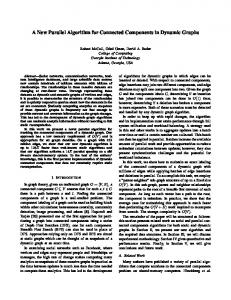
Figure 3 represents two different connected components as black pixels in a binary image along with their co-ordinates. The dashed arrows show the direction of scanning. Connected component-1 consists of black pixels at (7, 3), (8, 3), (7, 4) and (9, 4) co-ordinates. Connected component-2 consists of black pixels at (3, 4), (3, 5) and (4, 5) co-ordinates. A. Generation of tree While scanning we hit the first black pixel at coordinate (7, 3). So we create a node and store the corresponding row and column value i.e. 7 and 3.
P. Kumar, S. R. Giri, G. R. Hegde and K. Verma / IJECCT 2012, Vol. 2 (2)
29
Figure 4. Node for co-ordinate (7, 3)
Then we find all the 8-neighbourhood pixels of the current black pixel i.e. (7, 3). The neighbourhood pixels are (8,3) and (7,4). So we create two nodes and store the row and column values in the nodes. The nodes are linked with the current pixel node i.e. (7,3) as shown in figure 5. Figure 6.Linking of previous and current nodes for connected component-1
Figure 7.Tree containing all black pixels as nodes
Figure 5. The black pixels of connected component-1 in node format
Finally the tree is constructed. Now the next step is to group together all connected pixels. Let us name the nodes as demonstrated in figure 8.
We continue scanning in the same direction and hit the second black pixel (8, 3). Similarly we create a node for this pixel and link all the neighbourhood pixels with the pixel (8, 3). Finally we link the previous node with the current node as shown in figure 6.Similarly we create nodes for every black pixel, link them with their neighbourhood pixels and link them with each other. The final tree will be as depicted in figure 7. Figure 8. Nomenclature of nodes in the tree
First of all, compare Bottom of Current node with all Top nodes except Current. Thus we compare (8, 3) i.e. Bottom of (7,3) with Next of Current i.e. (8,3). Since it is equal, we merge Next of Current node with Current.
P. Kumar, S. R. Giri, G. R. Hegde and K. Verma / IJECCT 2012, Vol. 2 (2)
Then delete the node (8, 3) because it is a duplicate node. Duplicate nodes are removed before joining. Then compare all the Bottom nodes of Current including Top node of Current with all the nodes of Next of Current. When two nodes match, delete the node from Next of Current and there is no need to compare the same node of Current with other nodes of Next of Current. Thus the comparison is done as follows: (7, 3) – (7, 3) -> Matched. Thus delete (7,3) from Next of Current (8, 3) – (7, 4) -> Unmatched. So do not delete (7, 4) from Next of Current (8, 3) – (9, 4) -> Unmatched. So do not delete (9, 4) from Next of Current (7, 4) – (7, 4) -> Matched. Thus delete (7, 4) from Next of Current At the end, node (9, 4) is left in Next of Current. Now join (9, 4) with Current and update Bottom to Next of Bottom as shown in the following figure 9.
30
Figure 10.Final Tree structure for the connected components
These two sets represent two independent connected components. Now construct two separate images for these two sets. B. How to Create Separate Images with new co-ordinate values a) Find the minimum row and column values for Current. b) Find the maximum row and column values Current.
Figure 9. The intermediate tree
for
For this example max_row = 9, max_col = 4, min_row = 7 and min_col = 3. Create a 2D matrix of dimension [max_row – min_row +1] [max_col – min_col +1]. a) For a given co-ordinate (x,y) the new co-ordinate values will be [x – min_row + 1][y –min_col + 1] as shown in Figure 11.
Now compare Bottom of Current i.e. (7, 4) with Top node of Next of Current i.e. (3, 4). Since it is not matched, compare with next Top node i.e. (7, 4). It is matched. Do similar operations as explained before. When Bottom of Current reaches to Null, shift Current to Next of Current and set Next of Current. Do comparison as explained before. The final tree will be as shown in Figure 10.
Figure 11. New co-ordinates for the connected components
P. Kumar, S. R. Giri, G. R. Hegde and K. Verma / IJECCT 2012, Vol. 2 (2)
Now these new co-ordinate values will be filled with black pixels and a new image will be created from that matrix. Similarly a new image will be constructed for the second connected component. The final result will be in the form of two separate images as shown below.
Figure 12. The separated connected components
III. The SAGAP Algorithm The final algorithm of SAGAP to find the connected components in a binary image is presented below. 1. 2. 3. 4.
Read the binary image and store it in a matrix. Set Start node= Null. Set Root = Null. Read the matrix either row wise or column wise. If (black pixel found) a. Create a node (Top node) and store corresponding row and column value in that Top node. b. Set Bottom node = Top node.
31
column value of the neighbourhood black pixel. II. Set Bottom.Down = Temp node. III. Set Bottom node = Temp node. e. Repeat from Step- 4(c) to Step- 4(d) for every 8-neighbourhood black pixel. 5. End if 6. If (Start node = null) Set Start node = Top node. Set Root = Top node. Else Set Start. Right = Top node. Set Start node= Top node. 7. End if 8. Repeat from Step-3 to Step-6 until every black pixel of the matrix is visited. 9. Set Current = Root. 10. Set Bottom = Current. Down. 11. Set Next = Current. Right. 12. Do If (Bottom.row = Next.row) AND (Bottom.col = Next.col) a. Set Temp = Next. Set Next = Next. Down. Set Current. Right= Next. Set Next. Right=Temp.Right. Delete node Temp. b. Compare all nodes of Current with all nodes of Next. c. If (matched) d. Delete the duplicate node from Next and link accordingly. e. Join the remaining nodes (unmatched) of Next with Bottom and Set Current. Right=Next. Right. Else
Figure 13: Input image for SAGAP
Figure 14: Individual output sub-images from SAGAP
c. d.
Search for all 8-neighbourhood black pixels of the Top node. If (neighbourhood black pixel found) I. Create a new node (Temp) and store the corresponding row and
Set Next=Next. Right. 13. Set Bottom=Bottom. Down. Set Next = Current. Right. 14. Repeat Step 11 and Step 12 till Bottom reaches to Null. 15. Set Current=Current.Right.Set Bottom=Current. Down. Set Next=Current. Right. 16. Repeat from Step 11 to Step 14 until Next reaches to Null. V CONCLUSIONS AND FUTURE WORK We have developed a lucid and a novel algorithm called SAGAP to find connected components in a binary image of vehicle license plate. We have tested the
P. Kumar, S. R. Giri, G. R. Hegde and K. Verma / IJECCT 2012, Vol. 2 (2)
algorithm on fifty binary images of vehicles in Indian conditions of dimensions 3648 X 2736 pixels with connected components and found the algorithm to be 100% accurate with the average execution time of 1 to 1.5 seconds. The testing was done using a Intel® Core™2 Duo CPU with speed 2.20 GHz having 3GB RAM. The algorithm is a tad slower than some algorithms but nonetheless gives outstanding results. In the future we are interested to make the execution time faster so that it can be exploited further not only for this applications but also for other real-time applications in image processing. REFERENCES [1]
[2]
[3]
A. Rosenfeld and J. Plaftz, “Sequential operations in digital picture processing”, Journal of the ACM, 13(4), 471- 494 (1966). Christopher T Johnston and Donald G Bailey, “FPGA Implementation of a Single Pass Connected Components Algorithm”, 4th IEEE International Symposium on Electronic Design, Test & Applications,229-231 (2008). Fu Chang and Chun-Jen Chen, "A Fast Method for Labeling Connected Components in an image",16th IPPR Conference on Computer Vision, Graphics and Image Processing (CVGIP 2003).
32
Rafael C. Gonzalez and Richard E. Woods, “Digital Image Processing”, Second Edition , Prentice Hall India,2006. [5] Milan Sonka, Vaclav Hlavac and Roger Boyle, “Digital Image Processing and Computer Vision”,Cengage Learning, India Edition,2008 [6] Alasdair McAndrew, “Introduction to Digital Image Processing with MATLAB®”, Cengage Learning, India Edition,2004. [7] Yang, X.D., “An Improved Algorithm for Labeling Connected Components in a Binary Image,” TR 89-981,March 1989. [8] Tetsuo Asano and Hiroshi Tanaka, "In-place Algorithm for Connected Components Labeling", Journal of Pattern Recognition Research 1 (2010) 10-22. [9] Akmal Rakhmadi,N.Z.S Othman,Abdullah Bade,Mohd Shafry Mohd Rahim and Ismail Mat Amin, "Connected Component Labeling Using Components Neighbors-Scan Labeling Approach",Journal of Computer Science 6 (10):1070-1078,2010. [10] Jablonski, M., Gorgon, and M., "Handel-C implementation of classical component labelling algorithm", in Euromicro Symposium on Digital System Design (DSD 2004), Rennes, France, 387-393 (2004). [11] Jung-Me, P., C.G. Looney and C. Hui-Chuan, 2000, "Fast connected component labeling algorithm using a divide and conquer technique", Proceeding of the Conference on Computers and their Applications, Mar. 29-31, ISCA, New Orleans, USA., pp: 373-376. [4]