> TGRS-2015-01025.R2
1
A Novel Cluster Kernel RX Algorithm for Anomaly and Change Detection Using Hyperspectral Images Jin Zhou, Chiman Kwan, Senior Member, IEEE, Bulent Ayhan, and Michael Eismann
Abstract— The Reed-Xiaoli (RX) algorithm has been
widely used as an anomaly detector for hyperspectral images. Recently, kernel RX (KRX) has been proven to yield high performance in anomaly detection and change detection. In this paper, we present a generalization of KRX algorithm. The novel algorithm is called cluster kernel RX (CKRX), which becomes KRX under certain conditions. The key idea is to group background pixels into clusters and then apply a fast eigen-decomposition algorithm to generate the anomaly detection index. Both global and local versions of CKRX have been implemented. Application to anomaly detection using actual hyperspectral images is included. In addition to anomaly detection, the CKRX algorithm has been integrated with other prediction algorithms for change detection. Spatially-registered visible and near-infrared (VNIR) hyperspectral images collected from a tower-based geometry have been used in the anomaly and change detection studies. Receiver operating characteristics (ROC) curves and actual computation times were used to compare different algorithms. It was demonstrated that CKRX has comparable detection performance as KRX, but with much lower computational requirements. Index Terms— anomaly detection, change detection algorithms, hyperspectral imaging, RX, kernel RX, cluster kernel RX, ROC
I. INTRODUCTION
H
YPERSPECTRAL images have gained popularity in recent years. NASA’s Hyperion [1] has been operational since 2000. Moreover, NASA is also planning the HyspIRI mission [2], which will cover the whole Earth. Comparing to color (GeoEye) [3] and multi-spectral imagers in LANDSAT [4] that have only 3-10 bands, the hyperspectral Paper received on October 3, 2015, revised on January 5, 2016 and March 29, 2016, accepted on June 12, 2016. This work was supported in part by the Air Force Office of Scientific Research (AFOSR) under contract FA9550-09C-0162. J. Zhou is with Google, Inc., Mountain View, CA 80305 USA (e-mail: ferryzhou@ google.com). C. Kwan is with Signal Processing, Inc., Rockville, MD 20850 USA (email:
[email protected]). B. Ayhan is with Signal Processing, Inc., Rockville, MD 20850 USA (email:
[email protected]). M. Eismann is with the Air Force Wright Patterson Lab., Dayton, OH 45433 USA (e-mail:
[email protected]).
imagers offer hundreds of spectral bands. As a result, the discrimination power using hyperspectral imagers is significantly better than multi-spectral counterparts. Anomaly detection using hyperspectral images is important in many applications such as anomaly detection [5]-[7],[15][20], target detection [21],[22], change detection [10][13],[24],[25], rescue and search operations [14],[23], etc. A pixel is considered anomalous if it is different from its neighbors. A well-known anomaly detector is the Reed-Xiaoli (RX) algorithm [5]. There are several variants of the RX algorithms. Global RX uses statistics of background pixels in the whole image whereas local RX uses statistics from a small neighborhood of the test pixel. There is also the subspace RX (SSRX) where only certain principal eigenvectors are retained in the covariance matrix of the background pixels. A comparative study of various anomaly detection algorithm was given in [7]. A tutorial review on anomaly detection was provided in [8]. In [6], a new kernel RX (KRX) algorithm was proposed, which yielded excellent performance in anomaly detection as compared to both local and global RX. One limitation of KRX is that it is highly computationally demanding, which may limit its scope in real-time applications such as search and rescue operations. In this paper, we propose a fast generalization of KRX. The novel algorithm is called cluster kernel RX (CKRX), which becomes KRX under certain conditions. The key idea is to group background pixels into clusters and then apply a fast eigen-decomposition algorithm to generate the anomaly detection index. Both global and local versions of CKRX have been implemented. In addition to anomaly detection, the CKRX algorithm has been integrated with other prediction algorithms for change detection. Actual experimental data from a tower-based VNIR hyperspectral sensor were used in the detection studies. They were spatially-registered across collected images to allow change detection processing without the need for spatial registration pre-processing. Receiver operating characteristics (ROC) curves and actual computation times were used to compare different algorithms. It was demonstrated that CKRX has comparable detection performance as KRX, but with much lower computational requirements. Our paper is organized as follows. Section II first reviews RX and KRX. CKRX is then introduced. The complexity of CKRX is analyzed and an example is used to illustrate its performance and computational efficiency. Section III describes the application of CKRX to anomaly detection and it is shown that CKRX has comparable detection performance as KRX. In Section IV, a thorough comparative study is
> TGRS-2015-01025.R2
2
summarized for change detection using hyperspectral images. Change detection is cast as a two-stage process: prediction and anomaly detection. Several methods were compared in both the prediction and detection parts. It has been demonstrated that CKRX yielded comparable performance as that of KRX. Throughout this paper, a set of hyperspectral images collected by the US Air Force was used in our studies. These images have been used in [14]. For completeness, those images are summarized in the Supplementary Materials section.
1.
Construct
2.
Set μˆ b = μ = Kw where w is an M × 1 matrix with
ij
ˆ is the background covariance matrix estimated from where C b the reference background clutter data, and μˆ b is the estimated background clutter sample mean. Basically, the RX detector is based on the Mahalanobis distance between the pixel under test r and the background. In KRX, every pixel is transformed to a high dimensional space via a nonlinear transformation. The kernel representation for the dot product in feature space between two arbitrary vectors xi and x j is expressed as
k ( x i , x j ) = Φ ( x i ), Φ ( x j ) = Φ ( x i )iΦ ( x j ) A commonly used kernel is the Gaussian radial basis function (RBF) kernel k ( x, y ) = exp
(( − x − y ) / c ) 2
(2)
where c is a constant, x and y are spectral signatures of two pixels in a hyperspectral image. The above kernel function is the well-known kernel trick that avoids the actual computation of high dimensional features and enables the implementation of KRX.
i
j
each element w i = 1 / M . 3.
ˆ = K − μeT − eμ T + ew T μeT Set K
where e is an
M × 1 vector with ei = 1 .
4.
Perform singular ˆ = VDV T . K
5.
Cut D and V to a length of t. D = D(1 : t ,1 : t ) ,
II. CLUSTER KERNEL RX A. RX and KRX Given a single hyperspectral pixel as the observation test vector, the RX-algorithm is given by [6] T ˆ −1 ( r − μˆ ) RX(r ) = ( r − μˆ b ) C (1) b b
kernel matrix where K, K = k ( x , x ) and k is the kernel function (2).
value
decomposition
(SVD).
V = V (:,1 : t ) where D (t + 1, t + 1) < D (1,1) × 10
−8
T
6.
Set μ = μ − ew μ
7.
Set γ = γ − ew γ where γ i = k ( x i , r )
8.
Set v = D V
T
−1
T
( γ − μ)
2
The basic idea of CKRX is to first cluster background pixels and then replace each pixel with its cluster’s center. After replacement, the number of unique pixels is the number of clusters, which can be very small comparing to the original pixel set. Although the total number of pixels does not change, the computation of the anomaly value can be simplified using only the unique cluster centers, which improves the speed by several orders of magnitudes. The foundation behind this simplification is the following proposition. Proposition: Given a data set X which consists of disjoint clusters Sk ’s (k =1, 2, . . . ,m), each with cluster size |Sk | and cluster representative zk . For any two points xi ∈ Sp and xj ∈ Sq , the kernel evaluation k(xi , xj ) is approximated by using the corresponding cluster representatives as k(xi , xj )= k(zp, zq ). Now a block-wise constant matrix W is given by
Wij = k ( z p , z q ) , x i ∈ S p , x j ∈ S q , 1 ≤ i , j ≤ n , 1 ≤ p , q ≤ m (3)
B. CKRX KRX [6] is a generalization of the RX algorithm. When the kernel distance function is defined as the dot product of two vectors instead of (2), KRX is the same as RX. While KRX is more flexible than RX, it is significantly slower than RX. In this paper, we propose a novel algorithm which can perform fast approximation of KRX. The algorithm is based on clustering of background pixels. As a matter of fact, CKRX is a generalization of KRX, i.e. CKRX is reduced to KRX under some particular settings. To introduce CKRX, we start with KRX. The following description summarizes the KRX in details. Algorithm KRX Input: Given M background pixels: X b = [ x1 , x 2 , ⋯ , x M ] , a testing pixel r Output: The anomaly value v Algorithm:
Then ~ φ (i ) = φ (k ) , ∀xi ∈ S k
(4)
where φ (i ) is the i element of the eigenvector of W and ~ ɶ with φ (k ) is the kth element of eigenvector of the matrix W th
Wɶij = k ( z p , z q ) sq
(5)
where sq is the size of cluster Sq . That is, φ is obtained by repeating the kth entry of φɶ (1 ≤ k ≤ m )
sq times and then
concatenating them together. The proof of this proposition can be found in [9]. Based on this proposition, we propose the CKRX algorithm as follows: Algorithm CKRX Input: Background Xb = [ x1 , x 2 , ⋯ , x M ] , a testing pixel r Output: The anomaly value v Algorithm:
> TGRS-2015-01025.R2
3
1.
Perform clustering on Xb and get a set of clusters
2.
are center and size of ith cluster, respectively. Set v = WKRX ( C, r ) .
C = {( z1 , s1 ) , ( z 2 , s 2 ) , ⋯ , ( z m , s m )} where z i and si
WKRX is called weighted KRX and the algorithm is given by: Algorithm WKRX Input: Weighted points C = {( z1 , s1 ) , ( z 2 , s 2 ) , ⋯ , ( z m , s m )} , a testing point r Output: The anomaly value v Algorithm: 1. Construct kernel matrix K , where K ij = k ( z i , z j ) and k is the kernel function. m
2. Set μˆ b = μ = Kw where wi = si /
∑s
where m is the number of clusters. Suppose the original pixel number is n times of the cluster number, then the speed 3
boosting is n . To illustrate the computational efficiency and performance, Fig. 1 shows an example of CKRX applied to a synthetic data set. The data model is a mixture of Gaussians and there are 1000 points. The kernel is a Gaussian kernel. The color in the image corresponds to the log of the anomaly value. The results using KRX, KRX with sub-sampling, and CKRX are shown in (a), (b) and (c) respectively. The number of the original data points is 1000 and the data point number in both sub-sampled KRX and CKRX is 50. From the image, we can see that the CKRX provides better approximation than sub-sampled KRX. We also compared the speed of these three algorithms and the result is shown in Table 1. The eigen-decomposition of the kernel matrix in CKRX is about 1/2000 of that in original KRX, which is a huge speed improvement. Note this number is larger than theoretical 1/8000. This might be due to the CPU caching or compiler optimization issues.
i
i =1
ˆ = K − μeT − eμT + ew T μeT where e is an m × 1 3. Set K vector with ei = 1 .
ˆ 4. Perform eigen-decomposition. KSV = VD where S is ˆ is a diagonal matrix with Sii = si . Note that KS ɶ in the proposition. asymmetric which is similar to W 5. Cut D and V to a length of t. D = D(1 : t ,1 : t ) ,
V = V (:,1 : t ) where D(t + 1, t + 1) < D (1,1) × 10
−8
T
6. Set μ = μ − ew μ
Algorithm
T
8. Set v = D V
T
( γ − μ)
2
Construct Kernel Eigen-decomposition Anomaly detection
.
In the fourth step of WKRX, the eigenvalues and eigenvectors can be computed based on the following ˆ : transformation due to the asymmetric nature of KS ˆ KSV = VD 1
1
1
1
ˆ 2 S 2 V = S 2 VD ⇒ S 2 KS
(6)
ˆ 'V ' = V 'D ⇒K
Comparing WKRX with KRX, we can see that KRX is a special case of WKRX with si = 1 . We can also regard KRX as a special case of CKRX when each pixel is a cluster. In addition, we can treat KRX with background sub-sampling [18] as a special case of CKRX, in which each sampled point is the cluster center and each cluster has the same size. The complexity of CKRX is Ockrx = max(Oc , Owkrx ) (7) where Oc is the complexity of clustering and Owkrx is the complexity of WKRX. (8) Owkrx = O m 3
( )
Table 1: Comparison of the speed of KRX, KRX with sub-sampling, and CKRX. Time (s)
7. Set γ = γ − ew γ where γ i = k ( z i , r ) −1
(a) (b) (c) Fig. 1. Comparison of detection results using KRX, KRX with sub-sampling of background pixels, and CKRX. (a) shows the result of KRX using all data points, (b) shows the KRX results using 50 points, and (c) shows the results using CKRX results with 50 clusters. It can be seen that the results of CKRX is closer to KRX than that of KRX with sub-sampling, meaning that CKRX gives better detection.
KRX (1000 points)
KRX (50 points)
CKRX (50 clusters)
0.1590 4.6511 6.82
0.0038 0.0018 0.62
0.0030 0.0023 0.61
III. APPLICATION TO ANOMALY DETECTION In the Supplementary Materials section, which is also studied in [14], there are two images collected in October: one without targets and one with two small targets. For completeness and readability, we include the October image with targets in Fig. 2. We applied our CKRX algorithm to the October image with targets and also compared the anomaly detection results with KRX. The October image is preprocessed with Principal Component Analysis (PCA) transformation and only 10 bands are kept. More than 10 bands will not help the anomaly detection, as 10 bands already capture almost all the information content in the original hyperspectral data cube. Fig. 4 shows the comparison of KRX with background subsampling (2x2) and CKRX. The sub-sampling process is to speed up the KRX computations. Sub-sampling is also combined with a block pixel concept [18] where a block of 3x3 pixels share the same set of background pixels. The idea is that, instead of using a unique background for each single pixel, the block pixel method uses the same background for a block of pixels to compute the Mahalanobis distances, as Fig. 3 shows. Assuming the block pixel size is b x b, a further b2 time reduction can be achieved for both KRX and CKRX. A
> TGRS-2015-01025.R2
4
smoothing filter was used to smooth out the detection results. From Fig. 4, we can see that CKRX performs better than KRX with background sub-sampling while the speed of CKRX is even faster.
IV. APPLICATION TO CHANGE DETECTION A. RX and KRX Change detection involves two images [11][12]. Fig. 5 shows a simplified view of change detection, which has two parts: 1) Prediction/Transformation. Transform the original reference image (R) and testing image (T) to new space as PR and PT. 2) Change Evaluation. Evaluate the difference between the transformed image pair and output a single band detection image.
Fig. 2. Oct 14 image with 2 small targets inside the red circles.
Fig. 3. Illustration of using the same background for a block of pixels. The gray pixels are used as buffer between background pixels (yellow) and block pixels (red).
Fig. 5. Illustration of change detection between two images. R and T denote reference and test images, respectively.
B. Prediction Methods Prediction is important as the image contents between R and T may change significantly due to lighting conditions, weather conditions, seasonal changes, etc. Prediction will significantly improve the overall change detection performance. There are many prediction algorithms. Here, we include the following methods: 1. CC: Chronochrome [13] 2. CE: Covariance Equalization [10] 3. NN: Neural network (nonlinear approach) 4. Local methods: Local CC, CE, and NN.
krx krx
(a) ROC. X-axis denotes the false alarm rate and y-axis denotes the correct detection rate. Smooth means a 3x3 smoothing filter is applied to the detection results.
Algorithm CC [13] 1. Compute mean and covariance of R and T as mR ,
krx
2. 3.
C R , mT , CT Compute cross-covariance between R and T as CTR Do transformation. PR (i ) = CTR C R−1 (R (i ) − m R ) + mT , PT = T
Algorithm CE [10] 1. Compute mean and covariance of R and T as m R ,
C R , mT , CT
(b) Computational times comparison. Y-axis is time in seconds. “1” is the time using KRX and “2” is using CKRX. Fig. 4. Comparison of KRX with background subsampling (2x2) and CKRX. Both CKRX and KRX incorporated block pixel concept with a size of 3x3.
2.
Do eigen-decomposition (or SVD). C R = VR D RVRT ,
3.
CT = VT DT VTT Do transformation. PR (i ) = V R D R−1 / 2V RT (R (i ) − m R ) , PT (i ) = VT DT−1 / 2VTT (T (i ) − mT )
> TGRS-2015-01025.R2 Neural Network (NN) Similar to CC and CE, NN is used to capture the relationship/mapping between the reference and the testing image. We are the first ones to apply NN to capture the transformation between pixels in R and T for change detection. The NN is a standard two layer neural network with one layer of neurons and one layer of output weights. Since each pixel has a dimension of 10, there are 10 inputs and 10 outputs in the neural network. There is only one parameter in the neural network function: neuron_count. When neuron_count is 0, there is no hidden layer and the coefficient matrix dimension is 10 x 10. In this case, the neural network is a linear mapping and has similar performance as CC or CE. When neuron_count is non-zero, there is one hidden layer and one output layer. Therefore, the NN with hidden neutron layer can be considered as a nonlinear generalization of CC or CE methods. The coefficient matrix for the hidden layer is neuron_count × 10 and the coefficient matrix for the output layer is 10 × neuron_count. Each neuron is represented by a tansig function which is shown in Fig. 6.
Fig. 6. The function of a neuron.
Here we first summarize the local prediction algorithm. Fig. 7 illustrates the algorithm. Algorithm Local Prediction: Input: Reference image, testing image, block size b and window size w, a prediction function Output: Prediction image Algorithm: • Iterate over each non-overlapped block • Pick the corresponding window from reference image and testing image. Note that the prediction window size is larger than the non-overlapped block. • Perform prediction within the window • Fill the block in the predicting image. See Fig. 7.
Fig. 7. Local prediction idea.
5
C. Change Detection Methods After prediction, a residual image will be formed. Change detection will be carried by detecting the anomalies in the residual image. We have evaluated the following change detection algorithms: 1. ED: Euclidean distance fe ( v1 , v2 ) = v1 − v2 2.
AAD: Absolute f a ( v1 , v2 ) = avg ( v1 − v2 )
3.
VA: Vector angle. f v ( v1 , v2 ) = arccos
4.
NED: Normalized f n ( v1 , v2 ) = ( v1 − v2 ) / σ
5. 6. 7.
average
difference.
v1 × v2 T
v1 v2
Euclidean distance. where σ i is the variance
of the ith band of the difference image. RX [5]: Anomaly detection on the difference image. KRX [6]: Kernel RX (nonlinear anomaly detection algorithm) CKRX: Cluster KRX; faster than KRX
D. Post-processing to Generate Anomaly Detection Results After anomaly detection, there is an optional step, which is to smooth out the detection results so that false alarms may be reduced. We usually apply a simple 3x3 averaging filter. It will be seen in Section E that smoothing can help improve probability of detection and reduce false alarms. E. Change Detection Results Here, similar to Section 3, 10-band PCA transformed images were used for evaluation. Details about the hyperspectral images can be found in [14] and also in the Supplementary Materials section. One October image contains two small anomalies as shown in Fig. 2. The other images do not contain small anomalies. We can form 4 pairs: AugustOctober, September-October, October-October, and November-October. The window size in Fig. 7 is 21x21 and block size is 11x11. There are 4 rows in each one of Fig. 8, Fig. 9, and Fig. 10 with Aug indicating the Aug-Oct pair, Sept indicating the Sept-Oct pair, Oct indicating the Oct-Oct pair, and Nov indicating the Nov-Oct pair. Each row has 3 columns showing the residuals of 3 prediction methods: global, segmented, and local. Segmented means that the image is segmented into many sub-images and a global method is applied to each sub-image. This method was described in [14]. It can be seen from the figures, local prediction using CC, CE, and NN yields better performance (smaller residuals) as compared to their global counterparts. Dark pixels indicate smaller residuals in the figures. Fig. 11 shows change detection results using Local CC as the prediction algorithm and various detectors as the anomaly detection methods. There are 151 pixels on the two targets. The goal is to detect all the pixels. The image size is 800 x 1024. From the ROC curve shown in Fig. 11, we can see that about 10 false alarm pixels were picked up. All of the four AF image pairs in the Supplementary Materials section were used.
> TGRS-2015-01025.R2
6
As shown in Fig. 11, KRX and CKRX yielded the best performance. In particular, for a false alarm rate of 10-4, KRX and CKRX achieved more than 98% of probability of detection. Both local prediction and anomaly detection play important roles in change detection but the roles are different. Local prediction’s role is to detect non-changed pixels so that nonchanged pixels will not be interpreted as changed pixels. Anomaly detection’s role is to detect actual changed regions. Similar to prediction and anomaly detection, smoothing is also important. It is a post processing step and helps all methods. The smoothing can filter out noise, reduces false alarms, and thus improves the change detection results. From Fig. 11, it should be noted that even without smoothing, CKRX and KRX perform much better than RX.
Global NN (5 neurons)
Local NN (3 neurons)
Aug
Smaller residuals Sept
Oct
Nov Global CC
Segmented CC
Local CC
Aug
Smaller residuals
Fig. 10. Prediction residuals of global NN and local NN. First row: Aug and Oct image pair; Second row: Sept and Oct image pair; Third row: Oct and Oct image pair; Fourth row: Nov and Oct image pair. Blue pixels means small error and bright pixels means large errors. Local NN is better than global NN.
Sept
egmented CC
Oct
KRX and CKRX results
Nov
Fig. 8. Prediction residuals of global CC, segmented CC [14], and local CC. First row: Aug and Oct image pair; Second row: Sept and Oct image pair; Third row: Oct and Oct image pair; Fourth row: Nov and Oct image pair. Blue pixels means small error and bright pixels means large errors. Local CC has the smallest residuals as compared to global CC and segmented CC results. Global CE
Segmented CE
Local CE
Aug
Smaller residuals
Fig. 11. Comparison of ROC curves using different algorithms (KRX, CKRX, RX, etc.) Smooth means the detection results are smoothed by a 3x3 averaging filter. All methods are local in this plot. Local CC was used in the prediction step. X-axis: false alarm rate; y-axis: correct detection rate.
Sept
V. CONCLUSION
gmented CE Oct
Nov
Fig. 9. Prediction residuals of global CE, segmented CE [14], and local CE. First row: Aug and Oct image pair; Second row: Sept and Oct image pair; Third row: Oct and Oct image pair; Fourth row: Nov and Oct image pair. Blue pixels means small error and bright pixels means large errors. Local CE has the smallest residuals as compared to global CE and segmented CE results.
Although local KRX has much better performance local RX, its computation complexity limits its usage in real-time applications. A novel anomaly detector known as cluster kernel RX (CKRX) is proposed for processing hyperspectral images. The background pixels are grouped into clusters and the cluster centers are used in the anomaly detection process. The speed improvement is significant with almost no loss of detection performance. CKRX can be seen as a generalization of KRX from two perspectives. First, CKRX becomes KRX if every pixel is treated as a cluster. Second, since KRX is computationally intensive, background sub-sampling is normally applied to speed up the processing. KRX with background sub-sampling can be regarded as a special case of CKRX where each sampled point is a cluster and the cluster size is always fixed. Extensive evaluations have been performed to demonstrate the performance of CKRX in
> TGRS-2015-01025.R2 anomaly and change detection using actual hyperspectral images. ACKNOWLEDGMENT The imagery was provided by the Air Force Research Laboratory. The authors would also like to thank the anonymous reviewers who provided very detailed and constructive comments, which significantly improved the readability of our paper. REFERENCES [1] Hyperion, https://en.wikipedia.org/wiki/Earth_Observing-1 [2] HyspIRI, https://hyspiri.jpl.nasa.gov/ [3] GeoEye, https://en.wikipedia.org/wiki/GeoEye [4] Landsat, http://landsat.usgs.gov/ [5] I. S. Reed and X. Yu, “Adaptive multiple-band CFAR detection of an optical pattern with unknown spectral distribution,” IEEE Trans. Acoust., Speech Signal Process., vol. 38, no. 10, pp. 1760–1770, Oct. 1990. [6] H. Kwon, N.M. Nasrabadi, “Kernel RX-algorithm: A nonlinear anomaly detector for hyperspectral imagery,” IEEE Transactions on Geoscience and Remote Sensing, Vol.43, No.2, Feb 2005. [7] D. Borghys, I. Kasen, V. Achard, and C. Perneel, "Hyperspectral anomaly detection: Comparative evaluation in scenes with diverse complexity," Journal of Electrical and Computer Engineering, Special Issue on "Algorithms for Multispectral and Hyperspectral Image Analysis, 2012. [8] S. Matteoli, M. Diani, and G. Corsini, “A tutorial overview of anomaly detection in hyperspectral imagery,” IEEE Aerospace and Electronic Systems Magazine, Part 3: Tutorials, vol. 21, no. 3, June 2010. [9] K. Zhang and J. T. Kwok, “Density-weighted Nystrom method for computing large kernel eigen-systems,” Neural Comput. v21 i1. 121146. [10] A. Schaum and A. Stocker, “Hyperspectral change detection and supervised matched filtering based on covariance equalization,” Proc. SPIE, vol. 5425, pp. 77-90, 2004. [11] M. J. Carlotto, “Nonlinear background estimation and change detection for wide area search,” Opt. Eng., vol. 39, no. 5, pp. 1223–1229, [12] A. A. Nielsen, “The Regularized Iteratively Reweighted {MAD} Method for Change Detection in Multi- and Hyperspectral Data,” IEEE Transactions on Image Processing, vol. 16, No. 2, pp. 463-478, 2007. [13] A. Schaum and A. Stocker, “Long-interval chronochrome target detection,” presented at Int. Symp. Spectral Sens. Res., 1997. [14] J. Meola, Analysis of Hyperspectral Change and Target Detection as Affected by Vegetation and Illumination Variations (Masters Thesis, University of Dayton, Dayton, OH, 2006). [15] J. Zhou, C. Kwan, and B. Ayhan, “A High Performance Missing Pixel Reconstruction Algorithm for Hyperspectral Images,” 2nd. International Conference on Applied and Theoretical Information Systems Research, Taipei, Taiwan, December 27-29, 2012. [16] B. Ayhan, C. Kwan, X. Li, and A. Trang, “Airborne Detection of Land Mines Using Mid-wave Infrared (MWIR) and Laser-illuminated-near Infrared Images with the RXD Hyperspectral Anomaly Detection Method,” Fourth International Workshop on Pattern Recognition in Remote Sensing, Hong Kong, August 26, 2006. [17] L. He, J. Luo, H. Qi, and C. Kwan, “A Comparative Study of Several Unsupervised Endmember Extraction Algorithms to Anomaly detection in Hyperspectral Images,” International Symposium on Spectral Sensing Research, Missouri, July 2010. [18] J. Zhou and C. Kwan, “Fast Anomaly Detection Algorithms for Hyperspectral Images,” J. Multidisciplinary Engineering Science and Technology, Volume 2, Issue 9, September, 2015. [19] W. Wang, S. Li, H. Qi, B. Ayhan, C. Kwan, and S. Vance, “Identify Anomaly Component by Sparsity and Low Rank,” IEEE Workshop on Hyperspectral Image and Signal Processing: Evolution in Remote Sensor (WHISPERS), Tokyo, Japan, June 2-5, 2015. [20] S. Li, W. Wang, H. Qi, B. Ayhan, C. Kwan, and S. Vance, “Low-rank Tensor Decomposition based Anomaly Detection for Hyperspectral Imagery,” IEEE International Conference on Image Processing (ICIP), Quebec City, Canada, September 27-30, 2015. [21] D. Nguyen, T. Tran, C. Kwan, and B. Ayhan, “Endmember Extraction in Hyperspectral Images Using l-1 Minimization and Linear Complementary Programming,” Proc. SPIE, Vol. 7695, 2010.
7 [22] J. Zhou, C. Kwan, and B. Ayhan, “Hybrid In-Scene Atmospheric Compensation (H-ISAC) of Hyperspectral Images for High Performance Target Detection,” International Symposium on Spectral Sensing Research, Missouri, July, 2010. [23] B. Ayhan and C. Kwan, “Fast Target Detection Framework for Onboard Processing of Multispectral and Hyperspectral Images,” NASA HyspIRI Science Symposium, Greenbelt, Maryland, June 2015. [24] B. Ayhan, J. Zhou, and C. Kwan, “High Performance and Accurate Change Detection System for HyspIRI Missions,” NASA HyspIRI Science Symposium, May, 2012. [25] J. Zhou, B. Ayhan, C. Kwan, and M. Eismann, “New and Fast algorithms for Anomaly and Change Detection in Hyperspectral images,” International Symposium on Spectral Sensing Research, Missouri, July 2010.
Jin Zhou received his PhD in Computer Science and Engineering from the Arizona State University in 2009. He was with Signal Processing, Inc. between 2009 and 2013. He is now with Google. He has worked on many projects including video processing and speech processing, fault location in power networks, speech enhancement in noisy environments, compressed sensing, and hyperspectral image processing. Chiman Kwan (S’85-M’93-SM’98) received his BS with honors in Electronics from the Chinese University of Hong Kong in 1988, an MS and Ph.D. degree in electrical engineering from the University of Texas at Arlington in 1989 and 1993, respectively. Currently, he is the Chief Technology Officer of Signal Processing, Inc., leading research and development efforts in chemical agent detection, biometrics, speech processing, and fault diagnostics and prognostics. His primary research areas include fault detection and isolation, robust and adaptive control methods, signal and image processing, communications, neural networks, and pattern recognition applications. From April 1991 to February 1994, he worked in the Beam Instrumentation Department of the SSC (Superconducting Super Collider Laboratory) in Dallas, Texas, where he was heavily involved in the modeling, simulation and design of modern digital controllers and signal processing algorithms for the beam control and synchronization system. He later joined the Automation and Robotics Research Institute in Fort Worth, where he applied intelligent control methods such as neural networks and fuzzy logic to the control of power systems, robots, and motors. Between July 1995 and April 2006, he was with Intelligent Automation, Inc. in Rockville, Maryland. He has served as Principal Investigator/Program Manager for more than 100 different projects. Dr. Kwan has 8 patents, 29 invention disclosures, more than 65 papers in archival journals and more than 160 additional papers published in major conference proceedings. He is listed in the New Millennium edition of Who’s Who in Science and Engineering and is a member of Tau Beta Pi.
> TGRS-2015-01025.R2 Bulent Ayhan received his PhD in Electrical Engineering from the North Carolina State University in 12/2005. He worked at Intelligent Automation, Inc between 2006 and 2008. He joined Signal Processing, Inc. in November 2008. Dr. Ayhan involved in many projects, including chemical agent detection, fault diagnostics, data fusion, hyperspectral image processing, and speech processing.
Michael T. Eismann was born in Covington, Kentucky in 1964. He received a B.S. in Physics from Thomas More College in 1985, an M.S. in Electrical Engineering from the Georgia Institute of Technology in 1987, and a Ph.D. in Electro-Optics at the University of Dayton in 2004. From 1987 through 1996, he was employed by the Environmental Research Institute of Michigan (ERIM), where he was involved in research concerning active and passive electro-optical and infrared (EO/IR) targeting and reconnaissance sensors, optical information processing, and holographic optics. Since 1996, he has been performing electro-optical and infrared sensor research in the Sensors Directorate of the Air Force Research Laboratory (AFRL). He is the Senior Scientist for EO/IR Sensors, where he is responsible for overseeing the development of active and passive electro-optical and infrared sensor technology, and transition into operational airborne targeting and reconnaissance systems. He is also an Adjunct Assistant Professor at the Air Force Institute of Technology and Fellow of AFRL, SPIE, and the Military Sensing Symposia (MSS).
8
> TGRS-2015-01025.R2
9
Table 2 shows the five attributes of the hyperspectral images. These attributes are solar elevation (deg), solar azimuth (deg), date, collection time and weather conditions at the time of data collection. Fig. 12 shows the jpeg images of the 5 AF images. The pixel signatures of the four panels in each image are also shown in Fig. 12. In a related investigation, same pixels that belong to the same grass area have been picked from the 4 AF images and their signatures have been plot to visualize the variation in the signatures due to diurnal and seasonal changes. Fig. 13 shows the locations of the selected grass pixels in the four images separately. Fig. 14 shows the signatures of grass pixels in the four AF images. Table 2: Collection times and weather conditions for the 5 AF images. Image
Solar Elevation (deg)
Solar Azimuth (deg)
Date
Collection Time
Scene_180az_25_Aug_final.envi Scene_30el_1_Sept_final.envi
60.77 29.83
181.09 105.38
08/25/05 09/01/05
13:40:30 9:43:35
Scene_180az_14_Oct_final.envi
41.80
176.29
10/14/05
13:11:05
Scene_180az_14_Oct_change_final.envi Scene_30el_2_Nov_final.envi
41.73 30.47
184.99 151.39
10/14/05 11/02/05
13:37:20 10:38:45
Weather
Clear (some cirrus) Clear skies Partly cloudy with Haze Partly cloudy with Haze Clear
(a) Aug 25 (180 azimuth). 20 Panel1 (Black) Panel2 (Gre en) Panel3 (Tan ) Panel1 (Silver)
18 16
Amplitud e
14 12 10 8 6 4 2 0
20
40
60 Band no
80
100
120
(b) Four panel signatures in Aug 25 image (10 pixels each).
(c) Sep 1 (30 elevation). 20
Pan el1 (Black) Pan el2 (Green) Pan el3 (Tan) Pan el1 (Silver)
18 16 14 Amplitude
Supplementary Materials: Hyperspectral Images Used in this Paper We have used 5 hyperspectral images in this research for anomaly and change detection investigations. These 5 images were provided by United States Air Force. The image data were collected between August 2005 and November 2005. The collection instrument is a pan and tilt mounted VNIR Imaging Spectrometer with ~0.45 - 0.90 um wavelengths. For more information about the sensors, one should see [14]. There are a total of 5 hyperspectral imaging data files: • Scene_30el_1_Sept_final.envi Collected Sept. 1, 2005 with sun near 30 deg elevation angle • Scene_30el_2_Nov_final.envi Collected November 2, 2005 with sun near 30 deg elevation angle • Scene_180az_14_Oct_change_final.envi Collected Oct. 14, 2005 with sun near 180 deg azimuth (south). This image has small change targets inserted in the form of tarp bundles. • Scene_180az_14_Oct_final.envi Collected Oct. 14, 2005 with sun near 180 deg azimuth (south). This image was collected moments before the change file above. • Scene_180az_25_Aug_final.envi Collected Aug. 25, 2005 with sun near 180 deg azimuth (south).
12 10 8 6 4 2 0
20
40
60 Band no
80
100
120
(d) Four panel signatures in Sep 1 image (10 pixels each).
> TGRS-2015-01025.R2
10
(e) Oct 14 (180 azimuth).
(i) Nov 2 (30 elevation)
20
10 Pan el1 (Black) Pan el2 (Green) Pan el3 (Tan) Pan el1 (Silver)
18
8
14
7
12
6
Amplitude
Amplitude
16
Pan el1 (Black) Pan el2 (Green) Pan el3 (Tan) Pan el1 (Silver)
9
10 8
5 4
6
3
4
2
2
1
0
20
40
60 Band no
80
100
0
120
(f) Four panel signatures in Oct 14 image (10 pixels each).
20
40
60 Band no
80
100
120
(j) Four panel signatures in Nov 2 image (Panels are under shadow in Nov image) (10 pixels each). Fig. 12. Close look at the 5 AF images with signature plots of the four panels in the images.
(g) Oct 14 (targets in the red circles) (180 azimuth). 20 Panel1 (Black) Panel2 (Gre en) Panel3 (Tan ) Panel1 (Silver)
18 16
A mplitud e
14 12
Fig. 13. Grass pixels selected in four images (note that in Nov image the grass pixels are under shadow).
10 8
25
6 4
20
2 20
40
60 Band no
80
100
Sun near 1 80 degree azimu th Sun nea r 3 0 degree eleva tion Sun near 180 de gree a zimuth Sun nea r 3 0 degree elevation
120
(h) Four panel signatures in Oct 14(target) image (10 pixels each).
Amplitud e
0
Aug 2 5, Sep 1 , Oct 14, Nov 2 ,
15
10
5
0
20
40
60 Ban d no
80
100
120
Fig. 14 Signatures of grass pixels in 4 AF images (10 pixels each)