A Novel Feature Selection Approach Based on FODPSO and SVM

JOURNAL OF LATEX CLASS FILES, VOL. 6, NO. 1, JANUARY 2007

1

A Novel Feature Selection Approach Based on FODPSO and SVM Pedram Ghamisi, Student Member, IEEE, Micael S. Couceiro, Member, IEEE, Jon Atli Benediktsson, Fellow, IEEE

Abstract—A novel feature selection approach is proposed to address the curse of dimensionality and reduce the redundancy of hyperspectral data. The proposed approach is based on a new binary optimization method inspired by the FractionalOrder Darwinian Particle Swarm Optimization (FODPSO). The overall accuracy of a Support Vector Machine (SVM) classifier on validation samples is used as fitness values in order to evaluate the informativity of different groups of bands. In order to show the capability of the proposed method, two different applications are considered. In the first application, the proposed feature selection approach is directly carried out on the input hyperspectral data. The most informative bands selected from this step are classified by SVM. In the second application, the main shortcoming of using attribute profiles for spectral-spatial classification is addressed. In this case, a stacked vector of the input data and an attribute profile with all widely used attributes is created. Then, the proposed feature selection approach automatically chooses the most informative features from the stacked vector. Experimental results successfully confirm that the proposed feature selection technique works better in terms of classification accuracies and CPU processing time than other studied methods without requiring the number of desired features to be set a priori by users. Index Terms—Hyperspectral Image Analysis, Spectral-Spatial Classification, Attribute Profile, Feature Extraction, Random Forest Classifier, Automatic Classification.

I. I NTRODUCTION Hyperspectral remote sensors acquire a massive amount of data by obtaining many measurements, not knowing which data are relevant for a given problem. The trend for hyperspectral imagery is to record hundreds of channels from the same scene. The obtained data can characterize the chemical composition of different materials and potentially be helpful in analyzing different objects of interest. In the spectral domain, each spectral channel is considered as one dimension and each pixel is represented as a point in that domain. By increasing the number of spectral channels in the spectral domain, theoretical and practical problems may arise and conventional techniques which are applied on multispectral data are no longer appropriate for the processing of high dimensional data [1–3]. The aforementioned characteristics show that conventional techniques based on the computation of the fully dimensional P. Ghamisi and J. A. Benediktsson are with the Faculty of Electrical and Computer Engineering, University of Iceland, 107 Reykjavik, Iceland (corresponding author, e-mail: [email protected]) M. S. Couceiro is with Ingeniarius, Lda., and the Polytechnic Institute of Coimbra, 3030-199, Coimbra, Portugal. This research was supported in part by the Icelandic Research Fund for Graduate Students.

space, may not provide accurate classification results when the number of training samples is not substantial. For instance, while keeping the number of samples constant, after a few number of bands, the classification accuracy actually decreases as the number of features increases [1]. For the purpose of classification, these problems are related to the curse of dimensionality [4]. In order to tackle this issue and use a smaller number of training samples, the use of feature selection and extraction techniques would be of importance. From one point of view, feature selection techniques can be split into two categories: Unsupervised and supervised. Supervised feature selection techniques aim at finding the most informative features with respect to the available prior knowledge and lead to better identification and classification of different classes of interest. On the contrary, unsupervised methods are used in order to find distinctive bands when a prior knowledge of the classes of interest is not available. Information Entropy [5], First Spectral Derivative [6] and Uniform Spectral Spacing [7] can be considered as unsupervised feature selection techniques, while supervised feature selection techniques usually try to find a group of bands achieving the largest class separability. Class separability can be calculated by considering several approaches such as Divergence [8], Transformed divergence [8], Bhattacharyya distance [9] and Jeffries-Matusita distance [8]. A comprehensive overview of different feature selection and extraction techniques is provided in [10]. However, these metrics usually suffer from the following shortcomings: 1) They are usually based on the estimation of the second order statistics (e.g., covariance matrix) and in this case, they demand many training samples in order to estimate the statistics accurately. Therefore, in a situation when the number of training samples is limited, that may lead to the singularity of the covariance matrix. In addition, since the bands in hyperspectral data usually have some redundancy, the probability of the singularity will even increase. 2) In order to select informative bands, corrupted bands (e. g., water absorption bands and bands with a low SNR), are usually pre-removed, which is a time-consuming task. Furthermore, conventional feature selection methods can be computationally demanding. To select an m feature subset out of a total of n features, n!/(n−m)!m! operations must be calculated, which is a laborious task and demands a significant amount of computational memory. In other words, the conventional feature se-

JOURNAL OF LATEX CLASS FILES, VOL. 6, NO. 1, JANUARY 2007

lection techniques are only feasible in relatively low dimensional cases. In order to address the above-mentioned shortcomings of the conventional feature selection techniques, the use of stochastic and bio-inspired optimization based feature selection techniques (e.g., Genetic Algorithms (GA) and Particle Swarm Optimization (PSO)) are considered attractive. The main reasons behind this trend is that 1) in evolutionary feature selection techniques, there is no need to calculate all possible alternatives in order to find the most informative bands and furthermore, 2) in the evolutionary approaches, usually a metric is chosen as the fitness function which is not based on the calculation of the second order statistics, and, therefore, the singularity of the covariance matrix is not a problem. In the literature, there is an extensive number of works related to the use of evolutionary optimization based feature selection techniques. These methods are mostly based on the use of GA and PSO. For example, in [11], the authors proposed a SVM classification system which allows the detection of the most distinctive features and the estimation of the SVM parameters (e.g., regularization and kernel parameters) by using a GA. In [12], authors proposed to use PSO in order to select the most informative features obtained by morphological profiles for classification. In [13], in order to address the main shortcomings of GA- and PSO-based feature selection techniques and to take the advantage of their strength, a new feature selection approach is proposed, which is based on the hybridization of GA and PSO. In [14], a method was introduced which allows to simultaneously solve problems of clustering, feature detection, and class number estimation in an unsupervised way. However, this method suffers from the computational time required by the optimization process. In GA, if a chromosome is not selected for mating, the information contained by that individual is lost, since the algorithm does not have a memory of its previous behaviors. Furthermore, PSO suffers from the premature convergence of a swarm, because 1) particles try to converge to a single point, which is located on a line between the global best and the personal best positions, which this point does not guarantee to be a local optimum [15] and 2) furthermore, the fast rate of information flow between particles, can lead to the creation of similar particles. This results in a loss in diversity [16]. In this paper, a novel feature selection approach is proposed which is based on a new binary optimization technique and the SVM classifier. The new approach is capable of handling very high dimensional data even when only a limited number of training samples is available (ill-posed situation) and when conventional techniques are not able to proceed. In addition, despite the conventional feature selection techniques for which the number of desired features need to be initialized by the user, the proposed approach is able to automatically select the most informative features in terms of classification accuracy within an acceptable CPU processing time without requiring the number of desired features to be set a priori by users. The new feature selection technique is, at first, compared with the traditional PSO-based feature selection in terms of classification accuracy on validation samples and CPU processing time. Then, the new method is compared with a

2

few well-known feature selection and extraction techniques. Furthermore, the new method will be taken into account in order to overcome the main shortcomings of using attribute profiles. The rest of this paper is organized as follows: First, the new feature selection approach is described in Section II. Then, Section III briefly describes support vector machine. Section IV is devoted to the methodology of the proposed approach. Section V is on experimental results and main conclusion remarks are furnished in section VI. II. F RACTIONAL O RDER DARWINIAN PARTICLE S WARM O PTIMIZATION (FODPSO) BASED FEATURE SELECTION In brief, the goal is to overcome the curse of dimensionality [4] by selecting the optimal lE bands for the classification, lE ≤ l, wherein l is the total number of bands in a given image I. Selecting the most adequate bands is a complex task as the classification Overall Accuracy (OA) first grows and then declines as the number of spectral bands increases [4]. Hence, this paper tries to find the optimal lE bands that maximize the OA obtained as: PNc i Cii × 100, (1) OA = PN c i Cij wherein Cij is the number of pixels assigned to the class j which belongs to class i. Cii denotes the number of pixels correctly assigned to the class i and Nc is the number of classes. In this paper, optimal features are selected through an optimization procedure in such a way that each solution gets its fitness value from the SVM classifier over validation samples. The optimization procedure is handled with PSO algorithms. In 1995, Eberhart and Kennedy proposed the PSO algorithm for the first time [17]. The stochastic optimization ability of the algorithm is enhanced due to its cooperative simplistic mechanism, wherein each particle presents itself as a possible solution of the problem, e.g., the best lE bands. These particles travel through the search space to find an optimal solution, by interacting and sharing information with other particles, namely their individual best solution (personal best) and computing the global best [18]. The success of this algorithm gave rise to a chain of PSO-based alternatives in recent years, so as to overcome its drawbacks, namely, the stagnation of particles around suboptimal solutions. One of the proposed methods was denoted as Darwinian PSO (DPSO) [19]. The idea is to run many simultaneous parallel PSO algorithms, each one as a different swarm, on the same test problem and then a simple natural selection mechanism is applied. When a search tends to a suboptimal solution, the search in that area is simply discarded and another area is searched instead. In this approach, at each step, swarms that get better are rewarded (extend particle life or spawn a new descendent) and swarms that stagnate are punished (reduce swarm life or delete particles). For more information regarding how these rewards and punishments can be applied, please see [20]. DPSO has been investigated for the segmentation of remote sensing data in [21].

JOURNAL OF LATEX CLASS FILES, VOL. 6, NO. 1, JANUARY 2007

3

Despite the positive results retrieved by Tillett et al. [19], this coopetitive approach also increases the computational complexity of the optimization method. As many swarms of cooperative test solutions (i.e., particles) run simultaneously in a competitive fashion, the computational requirements increase and, as a consequence, the convergence time also increases. Therefore, and to further improve the DPSO algorithm, an extended version denoted as Fractional Order DPSO (FODPSO) was presented in [22], in which fractional calculus is used to control the convergence rate of the algorithm. This method has been further investigated for gray scale and hyperspectral image segmentation in [20, 23]. An important property revealed by fractional calculus is that, while an integer-order derivative just implies a finite series, the fractional-order derivative requires an infinite number of terms. In other words, integer derivatives are ”local” operators, while fractional derivatives have, implicitly, a ”memory” of all past events. The characteristics revealed by fractional calculus make this mathematical tool well suited to describe phenomena, such as the dynamic phenomena of particles’ trajectories. Therefore, supported on the FODPSO previously presented in [22], and based on the Grunwald Letnikov definition of fractional calculus, in each step t, the fitness function represented by (1) is used to evaluate the success of particles (i.e., OA). To model the swarm, each particle n moves in a multidimensional space according to the position (xn [t]), and velocity (vn [t]), values which are highly dependent on local best (˘ xn [t]) and global best (˘ gn [t]) information: vns [t + 1] =

(2)

wns [t + 1] + ρ1 r1 (˘ gns [t] − xsn [t]) + ρ2 r2 (˘ xsn [t] − xsn [t]), wns [t + 1] = (3) 1 1 αvns [t] + α(1 − α)vns [t − 1] + α(1 − α)(2 − α)vns [t − 2] 2 6 1 s + α(1 − α)(2 − α)(3 − α)vn [t − 3]. 24 Since the proposed FODPSO based feature selection approach is based on running many simultaneous swarms in parallel over the search space, ‘s’ shows the number of each swarm. The coefficients ρ1 and ρ2 are assigned weights, which control the inertial influence of ”the globally best” and ”the locally best”, respectively, when the new velocity is determined. Typically, ρ1 and ρ2 are constant integer values, which represent ”cognitive” and ”social” components with ρ1 + ρ2 < 2 [24]. However, different results can be obtained by assigning different values for each component. The fractional coefficient α, will weigh the influence of past events on determining a new velocity, 0 < α < 1. With a small α, particles ignore their previous activities, thus ignoring the system dynamics and becoming susceptible to get stuck in local solutions (i.e., exploitation behavior). On the other hand, with a large α, particles will have a more diversified behavior, which allows exploration of new solutions and improves the long-term performance (i.e., exploration behavior). However, if the exploration level is too high, then the algorithm may

take longer to find the global solution. Based on [24], a good α value can be selected in the range of 0.6 to 0.8. The parameters r1 and r2 are random vectors with each component generally a uniform random number between 0 and 1. In order to investigate FODPSO for the purpose of feature selection, the dimension of each particle should be equal to the number of features. In this way, the velocity dimension (dim vn [t]), as well as the position dimension (dim xn [t]), correspond to the total number of bands of the image, i.e., dim vn [t] = dim xn [t] = l. In other words, each particle’s velocity will be represented as a l-dimension vector. In addition, as one wishes to use the algorithm for band selection, each particle represents its position in binary values, i.e., 0 or 1, which 0 demonstrates the absence of the corresponding feature and 1 has a dual meaning. In this case, as proposed by Khanesar et al. [25], the velocity of a particle can be associated to the probability of changing its state as: ∆xn [t + 1] =

1

(4) 1+ Nevertheless, as one wishes to use the algorithm for band selection, each particle represents its position in binary values, i.e., 0 or 1. This may be represented as: ( 1, ∆xn [t + 1] ≥ rx xn [t + 1] = (5) 0, ∆xn [t + 1] < rx e−vn [t+1]

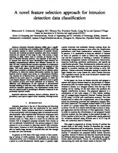
wherein rx is a random l-dimension vector with each component generally a uniform random number between 0 and 1. Therefore, each particle moves in a multidimensional space according to position xn [t] from the discrete time system represented by equations (2), (3), (4) and (5). In other words, each particle’s position will be represented as a l-dimensional binary vector. To make it easier to understand of the proposed strategy, an example is given in Fig. 1. As the figure shows, the image has only 5 bands, i.e., l=5. This means that each particle will be defined by its current velocity and position in the 5dimensional space, i.e., dim vn [t] = dim xn [t] = 5. In this example, and to allow a straightforward understanding, only a swarm of two particles was considered. As it is possible to observe at time/iteration t=1, particle 1 is positioned in such a way that it ignores the 4th band, i.e., x1 [1] = [1 1 1 0 1], while particle 2 ignores the 1st and 3rd bands i.e., x2 [1] = [0 1 0 1 1]. Computing (1) under those conditions returns an overall accuracy of OA1 = 60% and OA2 = 64% for particles 1 and 2, respectively. Considering only those two particles, particle 2 will be considered as the best performing one from the swarm, thus attracting particle 1 toward it. Such attraction will induce the velocity of particle 1 for iteration 2 and, consequently, its position. 1 III. S UPPORT V ECTOR M ACHINE (SVM) As discussed before, in the proposed method, the OA of SVM over validation samples is considered as the fitness 1 The MATLAB code for the PSO- and FODPSO-based feature selection approaches will be provided on a request by sending an email to the authors.

1, particle 1 is “positioned” in such a way that it ignores the 4th band, i.e., 𝑥1 [1] = [1 1 1 0 1], while particle 2 ignores the 1st and 3rd bands i.e., 𝑥2 [1] = [0 1 0 1 1]. Computing equation (1) under those conditions returns an overall accuracy of 𝑂𝐴1 = 60% and 𝑂𝐴2 = 64% for particles 1 and 2, respectively. Considering only those two particles, particle 2 will be considered as the best performing one from the swarm, thus attracting particle 1Atoward it. Such attraction will induce the velocity of particle 1 for iteration 2 and, JOURNAL OF LT X CLASS FILES, VOL. 6, NO. 1, JANUARY 2007 consequently, its position. E

𝑥1 [1] = [1

1

1

0

1]

𝑥2 [1] = [0

1

0

1

IV. METHODOLOGY

1]

Particle 1 is attracted toward particle 2 𝑏𝑎𝑛𝑑 = 5

In order to show the different capabilities of the proposed feature selection technique, two different scenarios have been taken into consideration.

𝑏𝑎𝑛𝑑 = 5

𝑏𝑎𝑛𝑑 = 4

𝑏𝑎𝑛𝑑 = 4

𝑏𝑎𝑛𝑑 = 3

𝑏𝑎𝑛𝑑 = 3

𝑏𝑎𝑛𝑑 = 2

𝑏𝑎𝑛𝑑 = 2

𝑏𝑎𝑛𝑑 = 1

𝑂𝐴1 = 60%

4

𝑏𝑎𝑛𝑑 = 1

𝑂𝐴2 = 64%

Particle 2 is the best!

Fig. X: Band coding of two particle for an image with 5 bands. Gridded bands are ignored in the classification process (equation 1).

Fig. 1. Band coding of two particles for an image with 5 bands. Gridded bands are ignored in the classification process.

References [1] G. Hughes, “On the mean accuracy of statistical pattern recognizers,” IEEE Trans. Inf. Theory, vol. IT, no. 14, pp. 55 – 63, 1968. [2] L. Breiman, “Random forests,” Mach. Learn., vol. 45, no. 1, pp. 5–32, 2001. [3] L. Breiman, “RF tools A class of two eyed algorithms,” in SIAM Workshop, 2003 [Online]. Available: http://oz.berkeley.edu/users/ breiman/siamtalk2003.pdf. [4] J. Kennedy and R. Eberhart, "A new optimizer using particle swarm theory," in in proceedings of the IEEE Sixth International Symposium on Micro Machine and Human Science, Nagoya , Japan, 1995. [5] Valle, Y. d., Venayagamoorthy, G. K., Mohagheghi, S., Hernandez, J. C., & Harley, R. (2008). Particle swarm optimization: Basic concepts, variants and applications in power systems. IEEE Transactions on Evolutionary Computation, 2(2), 171-195. [6] J. Tillett, T. M. Rao, F. Sahin, R. Rao and S. Brockport, "Darwinian Particle Swarm Optimization," in in proceedings of the 2nd Indian International Conference on Artificial Intelligence, 2005.

value. SVM has attracted much attention due to its capability of handling the curse of dimensionality in comparison with conventional classification techniques. The main reasons behind success of the approach are 1) SVM is based on a margin maximization principle which helps it to avoid estimating the statistical distributions of different classes in the hyperdimensional feature space and 2) SVM takes advantage of the strong generalization capability obtained by its sparse representation of the decision function [11].

In hyperspectral image analysis, the Random Forest (RF) classifier and SVM play a key role since they can handle high dimensional data even with a limited number of training samples. In this work, we prefer to use SVM rather than RF due to its susceptibility to noise. Due to its sensibility, corrupted and noisy bands may significantly influence on the classification accuracies. As a result, when RF is considered as the fitness function, due to its capability to handle different types of noises, corrupted bands cannot be eliminated even after high number of iterations. On the contrary, since SVM is more sensible than RF against noises, SVM can detect and eliminate corrupted bands after a few iterations, which can be considered as a privilege for the final classification step. The general idea behind SVM is to separate training samples belonging to different classes by tracing maximum margin hyperplanes in the space where the samples are mapped [26]. SVMs were originally introduced for solving linear classification problems. However, they can be generalized to nonlinear decision functions by considering the so-called kernel trick [27]. A kernel-based SVM is being used to project the pixel vectors into a higher dimensional space and estimate maximum margin hyperplanes in this new space, in order to improve linear separability of data [27]. The sensitivity to the choice of the kernel and regularization parameters can be considered as the most important disadvantages of SVM. The latter is classically overcome by considering cross-validation techniques using training data [28]. The Gaussian radial basis function (RBF) is widely used in remote sensing [27]. More information regarding SVM can be found in [29, 30].

A. First scenario In the first scenario, the new feature selection approach is directly performed on raw data sets in order to select the most informative bands from the whole data set. The main work flow of the proposed method for this scenario is listed below: 1) Training samples are split into two categories: Training and validation samples. 2) FODPSO-based feature selection is performed on the raw data. SVM is chosen as the fitness function and its corresponding OA is considered as the fitness value. 3) The selected bands are classified by SVM with the whole training and test samples and final classification map will be achieved. B. Second scenario In the second scenario, an application of the proposed FODPSO-based feature selection technique will be shown. In this scenario, we address the main shortcomings of using Attribute Profile (AP): 1) which attributes should be taken into account and 2) which values should be opted as threshold values. A comprehensive discussion related to AP and its all modifications and alternatives, can be found in [31]. In this scenario, different types of attributes with the wide ranges of threshold values will be constructed for building a feature bank and then, we let the proposed feature selection technique choose the most informative features from the bank with respect to the classification accuracy for the validation samples. In other words, the new feature selection technique not only solves the main shortcomings associated with the concept of AP, but also reduces the redundancy of the features and addresses the curse of dimensionality. Fig. 2 illustrates the flowchart of the proposed method based on FODPSO feature selection technique for the second scenario. The main work flow of this method is listed below: 1) A feature bank is made, consisting of raw input data and an AP obtained with four attributes with a wide range of threshold values. • The raw input data are transformed by Principal Component Analysis (PCA). • The most important Principal Components (PCs), i.e., components with cumulative variance of more than 99%, are kept and used as base images for the Extended Multi-AP (EMAP). • The obtained EMAP and the raw input data are concatenated into a stacked vector (let us call the output of this step ℘). 2) Training samples are split into two categories: Training and validation samples. 3) FODPSO based feature selection is performed on ℘. The fitness of each particle is evaluated by the OA of SVM for the validation samples. After a few iterations,

JOURNAL OF LATEX CLASS FILES, VOL. 6, NO. 1, JANUARY 2007

5

Fig. 3. The AVIRIS Hekla data set. a) Spectral band number 50; b) training samples, c) test samples, where each color represents a specific information class. The information classes are listed in Table I. Fig. 2. General idea of the proposed classification framework based on FODPSO-based feature selection technique for the second scenario.

the FODPSO based feature selection approach finds the most informative bands with respect to the OA of SVM over the validation samples (the output of this step will be called =). 4) = is classified by SVM by considering the whole set of training and test samples and a final classification map will be achieved. It should be noted that, in this work, the PCA can be replaced by other feature extraction techniques (in particular Kernel PCA and NWFE which have shown promising results in order to produce attribute profiles [31]). Now, a brief discussion on AP is given. 1) Extended Multi-Attribute Profile (EMAP): In order to overcome the shortcomings of the morphological profile, AP was introduced in [32] for extracting spatial information of the input data, which is based on attribute filters. APs can be regarded as more effective filters than morphological profiles because the concept of the attribute filters is not limited to only the size of different objects and the APs are able to characterize other characteristics such as shape of existing objects in the scene. In addition, APs are computed according to an effective implementation based on max-tree and min-tree representations, which lead to a reduction of the computational load when compared with conventional profiles built with operators by reconstruction. An AP is built by the sequence of attribute thinning and thickening transformations defined with a sequence of progressively stricter criteria [32]. To handle hyperspectral images, the extension of AP was proposed in [33]. Extended AP (EAP) is a stacked vector of different APs computed on the first C features extracted from the original data set. When different attributes, a1 , a2 , ..., aM are concatenated into a stacked vector, the EMAP is obtained. More information regarding AP and its different variations can be found in [2, 3, 31, 32]. In this paper, the following attributes have been taken into account: 1) (a) area of the region (related the size of the regions), 2) (s) standard deviation (as an index for showing the

Fig. 4. The AVIRIS Indian Pines data set. a) Spectral band number 27 (λ = 646.72µ); b) training samples, c) test samples, where each color represents a specific information class. The information classes are listed in Table II.

homogeneity of the regions), 3) (d) diagonal of the box bounding the regions, 4) (i) moment of inertia (as an index for measuring the elongation of the regions). V. EXPERIMENTAL RESULTS A. Data Description 1) Hekla data: The first hyperspectral data set used was collected on June 17, 1991 by AVIRIS (having spatial resolution 20 m) from the volcano Hekla in Iceland (see Fig. 3). Sixty four bands (from 1.84 µ to 2.4 µ) were removed due to the technical problem with the 4th spectrometer in 157 bands. An image of size 500 × 200 was used in this paper for the real experiments. For this data set, from the total number of training samples which is equal to 966, 50 percent was chosen for training and the rest as validation samples, in order to perform the PSO- and FODPSO-based feature selection approaches. After finding the most informative bands with respect to the OA of SVM over validation samples, all 966 samples are used for training in order to perform SVM on the selected bands. The number of training, validation and test samples are displayed in Table I. 2) Indian Pines data: The second data set used in experiments is the well-known data set captured on Indian Pines (NW Indiana) in 1992 comprising 16 classes (see Fig. 4), mostly related to different land covers. The data set consists of 145 × 145 pixels with spatial resolution of 20 m/pixel. In this

JOURNAL OF LATEX CLASS FILES, VOL. 6, NO. 1, JANUARY 2007

6

TABLE I H EKLA : NUMBER OF TRAINING , VALIDATION AND TEST SAMPLES . F OR THE FINAL CLASSIFICATION STEP, THE TOTAL OF TRAINING AND VALIDATION SAMPLES IS USED TO TRAIN THE SVM. Class Number

Name

1 2 3 4 5 6 7

Andesite lava 1970 Andesite lava 1980 I Andesite lava 1991 I Andesite lava moss cover Hyaloclastite formation Rhyolite Firn-glacier ice

Number of Samples Training Validation Test 97 54 150 49 38 20 76

97 54 150 49 38 19 75

829 442 1196 370 334 143 549

TABLE II INDIAN PINES: NUMBER OF TRAINING , VALIDATION AND TEST SAMPLES . F OR THE FINAL CLASSIFICATION STEP, THE TOTAL OF TRAINING AND VALIDATION SAMPLES IS USED TO TRAIN THE SVM. Class Number

Name

1 2 3 4 5 6 7 8 9 10 11 12 13 14 15 16

Corn-notill Corn-mintill Corn Grass-pasture Grass-trees Hay-windrowed Soybean-notill Soybean-mintill Soybean-clean Wheat Woods Bldg-Grass-Tree-Drives Stone-Steel-Towers Alfalfa Grass-pasture-mowed Oats

Number of Samples Training Validation Test 25 25 25 25 25 25 25 25 25 25 25 25 25 8 8 8

25 25 25 25 25 25 25 25 25 25 25 25 25 7 7 7

1384 784 184 447 697 439 918 2418 564 162 1244 330 45 39 11 5

work, 220 data channels (including all noisy and atmospheric absorbed bands) are used. In the same way, for Indian Pines, from the total number of training samples which is equal to 695, 50 percent of the samples were chosen for training and the rest for the validation samples, in order to perform the PSO- and FODPSO-based feature selection approaches. After performing PSO- and FODPSO-based feature selection approaches, all 695 samples are used for training in order to perform SVM on the selected bands. The number of training, validation and test samples are displayed in Table II. In this work, in addition to selecting data sets that are widely used in the hyperspectral imaging community, we have used exactly the same training and test samples that have been considered in most works related to the classification of hyperspectral images. Some of the works which have considered exactly the same training and test samples are given in references [3, 34]. In other words, we not only used the same number of training and test samples adopted by other state-ofthe-art methods, but the samples also have exactly the same spatial locations in the data. This way of using the training and test samples makes this work fully comparable with other spectral and spatial classification techniques reported in the literature.

B. General Information The following measures are used in order to evaluate the performance of different classification methods. 1) Average Accuracy (AA): This index shows the average value of the class classification accuracy. 2) Overall Accuracy (OA): This index represent the number of samples which is classified correctly divided by the number of test samples. 3) Kappa Coefficient (k): This index provides information regarding the amount of agreement corrected by the level of agreement that could be expected due to chance alone. 4) CPU Processing Time: This measure shows the speed of different algorithms. It should be noted, since in all algorithms (except Raw), EMAP is carried out, the CPU processing time of this step is discarded from all methods. Hence, the CPU processing time is only provided for AP, Raw + AP, Decision Boundary Feature Extraction (DBFE) and NWFE. Except DBFE and NWFE, which have been used in the MultiSpec software, all methods used were programmed in MATLAB on a computer having Intel(R) Pentium(R) 4 CPU 3.20 GHz and 4GB of memory. The number of iterations in each run for PSO- and FODPSO-based feature selection techniques is equal to 10. Since PSO- and FODPSO-based feature selection techniques are randomized methods which are based on different first populations, each algorithm has here been run 30 times and results are shown in different histograms and compared with different indexes in order to examine the capabilities of PSOand FODPSO-based feature selection techniques. It should be noted that, in this paper, in order to compare PSO and FODPSO, both data sets (Hekla and Indian Pines) have been taken into account. However for the first and second scenarios, we preferred to use only Indian Pines since this data set is more complex for classification. Therefore, the capability of the proposed method can be shown more clearly by using Indian Pines instead of Hekla. In this case, 25 PCs with a cumulative variance of more than 99% were selected as the base images for producing EMAP for Indian Pines. Based on [24], the sum of all ρ’s should be inferior to 2 and alpha should be near 0.632. Therefore, the parameters ρ1 , ρ2 and α are initialized by 0.8, 0.8 and 0.7, respectively. It should be noted that, the same set of parameters have been used for both data sets and both scenarios, in order to show that the proposed technique is data set distribution independent, and with the same set of parameters, for all different data sets and scenarios, the proposed method can lead to an acceptable results in terms of accuracies and CPU processing time. After comparing PSO- and FODPSO-based feature selection techniques in terms of overall accuracy over validation samples, the best method will be chosen for further evaluation. Then, the best method will be compared with the other wellknown feature selection and extraction techniques. In order to have a fair comparison, among 30 runs, four runs have been chosen and their classification accuracies are compared with obtained results from the other feature selection and extraction techniques. In this way, the results of 30 runs have been sorted in an increasing order with respect to their overall accuracy

JOURNAL OF LATEX CLASS FILES, VOL. 6, NO. 1, JANUARY 2007

over validation samples. Then, for a fair comparison with the other methods, the four runs are selected as follows: 1) Min: SVM classification is applied on the bands selected with the least overall accuracy over the validation samples among 30 runs (the first group of the most informative bands when the results of 30 runs have been sorted in an increasing order). 2) M edian1 : SVM classification is applied on the bands selected with the median overall accuracy over the validation samples among 30 runs (the 15th group of the most informative bands when the results of 30 runs have been sorted in an increasing order). 3) M edian2 : SVM classification is applied on the the most informative bands selected with the median overall accuracy over the validation samples among 30 runs (the 16th group of bands when the results of 30 runs have been sorted in an increasing order). 4) Max: SVM classification is applied on the bands selected with the highest overall accuracy over the alidation samples among 30 runs (the 30th group of the most informative bands when the results of 30 runs have been sorted in an increasing order).

7

above) and 2) the top few eigenvalues which account for 99% of the total sum of the eigenvalues were selected. The data sets have been classified with SVM and a Gaussian kernel. Five-fold cross validation is taken into account in order to select the hyperplane parameters when SVM is used for the last step (for the classification of informative bands). C. FODPSO vs. PSO

Other methods for the purpose of comparison are listed below: 1) Raw: The input data are directly classified with SVM without performing any feature selection or extraction technique. 2) Div: Divergence feature selection is performed on the input data and the selected bands are classified by SVM. 3) TD: Transformed Divergence feature selection is performed on the input data and the selected bands are classified by SVM. 4) Bhathacharyya: Bhathacharyya distance feature selection is performed on the input data and the selected bands are classified by SVM. 5) DBFE: DBFE is performed on the input data and the selected bands are classified by SVM. 6) NWFE: NWFE is performed on the input data and the selected bands are classified by SVM, and for the second scenario, 1) AP: The feature bank including all four attributes with a wide range of threshold values is classified by SVM. 2) Raw+AP: The Raw and AP are concatenated into a stacked vector and classified by SVM. The following ranges for different attributes have been taken into account in order to build the feature bank: a = ( 1000 phi ) × {1, 2, 3, 4, 5, 6, 7, 8, 9, 10, 11, 12, 13, 14} µ s = ( 100 ) × {5, 10, 15, 20, 25, 30, 35, 40, 45, 50} d = {10, 20, 30, 40, 50, 60, 70, 80, 90, 100} i = {0.1, 0.2, 0.3, 0.4, 0.5, 0.6, 0.7, 0.8, 0.9} where phi and µ are the resolution of the image in meters and the mean of a feature, respectively. Again, in order to secure the fairness of the comparison, the number of features for DBFE and NWFE has been chosen in 2 different ways: 1) the number of selected features is equal to the number of features which provides M ax (see a few lines

Fig. 5. Hekla: Box plots for overall accuracy over 30 runs for PSO-based feature selection (top) and FODPSO-based feature selection (bottom).

1) Hekla: Fig. 5 shows the box plots for the OA of the classification for 30 runs (10 iterations within each run) for PSOand FODPSO-based feature selection approaches, respectively. As can be observed from Fig. 5, although one cannot perceive any major differences between both methods, the FODPSObased feature selection approach presents an overall smaller interquartile range, i.e., the OA of the classification, at each run, has less dispersion regardless of the number of trials. On the other hand, the average value of the OA is slightly larger than for the PSO-based method. One-way MANOVA analysis was carried out to assess whether both the PSO- and FODPSO-based algorithms have a statistically significant effect on the classification performance. The significance of the different types of algorithm used (independent variable) on the final OA and the CPU processing time (dependent variables) was analyzed using one-way MANOVA after checking the assumptions of multivariate normality and homogeneity of variance/covariance, for a significance level of 5%. The assumption of normality of each of the univariate dependent variables was examined using a paired-sample Kolmogorov-Smirnov (p − value < 0.05) [35]. Although the univariate normality of each dependent variable has not been

trial graphically using boxplot charts (Fig. 1). The ends of the blue boxes and the horizontal red line in between correspond to the first and third quartiles and the median values, respectively. As one may observe, by benefiting from the fractional version of the algorithm, one is able to slightly increase the OA while, at the same time, slightly decrease JOURNAL OF LATEX CLASS FILES, VOL. 6, NO. 1, JANUARY 2007 the CPU processing time.

8

98.5

800

Processing time (sec)

98

97.5

700 600 500 400

Indian Pines.xlsx 300

PSO

Algorithm

FODPSO

PSO

Algorithm

FODPSO

Fig. 6. Hekla: Final classification accuracy in percentage and processing time in seconds for the PSO- and FODPSO-based feature selection approaches.

verified, since n ≥ 30 and this was assumed by benefiting from using the Central Limit Theorem (CLT) [36, 37]. Consequently, the assumption of multivariate normality was validated [37, 38]. Note that MANOVA makes the assumption that the within-group covariance matrices are equal. Therefore, the assumption about the equality and homogeneity of the covariance matrix in each group was verified with the Box’s M Test (M = 72.7642, F (3; 720) = −2.0706; p − value = 1.0000) [38]. The MANOVA analysis revealed that the type of algorithm did not lead to a statistically significant different outcome for the multivariate composite (F (1; 58) = 3.5830; p − value = 0.1667). In this situation, the FODPSO-based solution produces slightly better solutions than the PSO but is considerably faster than the latter. To easily assess the differences between both algorithms, let us graphically show the outcome of each trial using box plot charts (Fig. 6). The ends of the blue boxes and the horizontal red line in between correspond to the first and third quartiles and the median values, respectively. As one may observe, by benefiting from the fractional version of the algorithm, one is able to slightly increase the OA while, at the same time, slightly decrease the CPU processing time. 2) Indian Pines: Fig. 7 shows the box plots for the OA of the classification for 30 runs (10 iterations within each run) for PSO- and FODPSO-based feature selection approaches, respectively. Similarly as before, despite the lack of major differences, the FODPSO-based feature selection approach presents an overall smaller interquartile range and larger average value of the overall accuracy. Once again, one-way MANOVA analysis was carried out to assess whether both PSO- and FODPSO-based algorithms have a statistically significant effect on the classification performance. The assumption about the equality and homogeneity of the covariance matrix in each group was verified with the Box’s M Test (M = 72.5156, F (3; 720) = −2.0636; p − value = 1.0000). For this data set, the MANOVA analysis revealed that the type of the feature selection algorithm led to a statistically significant different outcome on the multivariate composite (F (1; 58) = 14.6338; p − value < 0.0001). As the MANOVA detected significant statistical differences, we proceeded to the commonly-used ANOVA for each dependent variable. By carrying an individual test on each dependent variable, it was possible to observe that the OA does not present statistically significant differences (F (1; 58) = 0.0116;

A one-way MANOVA analysis was carried out to assess whether both PSO- and FODPSO-based algorithms have a statistically significant effect on the classification performance. The significance of the different type of algorithm used (independent variable) on the final overall accuracy (OA) and the CPU processing time (dependent variables) was analyzed using a one-way MANOVA after checking the assumptions of multivariate normality and homogeneity of variance/covariance, for a significance level of 5%. The assumption of normality of each of the univariate dependent variables was examined using a paired-sample Kolmogorov-Smirnov (p-value < 0.05) [1]. Although the univariate normality of each dependent variable has not been verified, since 𝑛 ≥ 30 and using the Central Limit Theorem (CLT) [2] this statement was assumed [3]. Consequently, the assumption of multivariate normality was validated [3]. Note that MANOVA makes the assumption that the within-group covariance matrices are equal. Therefore, the assumption about the equality and homogeneity of the covariance matrix in each group was verified with the Box’s M Test (𝑀 = 72.5156, 𝐹(3; 720) = −2.0636; 𝑝 − 𝑣𝑎𝑙𝑢𝑒 = 1.0000). This suggests that the design is balanced and, since there is an equal number of observations in each cell (𝑛 = 30), the robustness of the MANOVA tests is guaranteed. The MANOVA analysis revealed that the type of algorithm led to a statistically significant different outcome on the multivariate composite (𝐹(1; 58) = 14.6338; 𝑝 − 𝑣𝑎𝑙𝑢𝑒 < 0.0001). As the MANOVA detected significant statistical differences, we proceeded to the commonly-used ANOVA for each dependent variable. By carrying an individual test on each dependent variable, it was possible to observe that the OA does not present statistically significant differences (𝐹(1; 58) = 0.0116; 𝑝 − 𝑣𝑎𝑙𝑢𝑒 = 0.9145). On the other hand, it is in the CPU processing time that both algorithms diverge the most, thus resulting in statistically significant differences between them (𝐹(1; 58) = 16.7499; 𝑝 − 𝑣𝑎𝑙𝑢𝑒 < 0.0001). As expected, the FODPSO-based solution produces slightly better solutions than the PSO considerably faster than the later. To easily assess the differences between both algorithms, let us show the outcome of each graphically using boxplot charts (Fig. 1). The ends of the blue boxes and the Fig. 7.trialIndian Pines: Box plots for overall accuracy in percentage over 30 runs horizontal red line in between correspond to the first and third quartiles and the median for PSO-based feature (top)byand FODPSO-based feature values, respectively. As selection one may observe, benefiting from the fractional versionselection of the (bottom). algorithm, one is able to increase the OA while, at the same time, decrease the CPU processing time. 320

72 300

71

Processing time (sec)

97

Classification accuracy (%)

Classification accuracy (%)

900

70 69 68 67 66 65

280 260 240 220 200 180 160

64

140

PSO

Algorithm

FODPSO

PSO

Algorithm

FODPSO

Fig. 8. Indian Pines: Final classification accuracy in percentage of the PSOand FODPSO-based feature selection approaches.

p − value = 0.9145). On the other hand, it is in the CPU processing time that both algorithms diverge the most, thus resulting in statistically significant differences between them (F (1; 58) = 16.7499; p − value < 0.0001). As expected, the FODPSO-based solution produces slightly better solutions than the PSO considerably faster than the latter. To easily assess the differences between both algorithms, the outcome of each trial is shown graphically using box plot charts (Fig. 8). As one may observe, by benefiting from the fractional version of the algorithm, one is able to slightly increase the OA (slightly higher median value) while, at the same time, considerably decrease the CPU processing time. D. First Scenario Fig. 9 shows the list of the selected bands by the proposed method in 30 different runs. Runs 2, 16, 30 and 29 are selected as Min, M edian1 , M edian2 and Max, respectively. As it was mentioned before, since the FODPSO-based feature selection technique is a randomized method which is based on different

JOURNAL OF LATEX CLASS FILES, VOL. 6, NO. 1, JANUARY 2007

9

TABLE III F IRST SCENARIO : T HE CLASSIFICATION OF DIFFERENT TECHNIQUES IN PERCENTAGE FOR I NDIAN P INES . T HE NUMBER OF FEATURES IS SHOWN IN BRACKETS . T HE BEST ACCURACY IN EACH ROW IS SHOWN IN BOLD .

Class No. 1 2 3 4 5 6 7 8 9 10 11 12 13 14 15 16 AA OA K Time

Raw (220) 54.1 57.5 80.4 88.3 81.4 92.2 68.0 49.1 64.1 95.6 79.0 64.5 95.5 64.1 81.8 100 76.02 65.41 0.6119 94

Min (84) 67.1 67.6 82.0 92.6 85.2 92.9 73.7 47.7 73.7 96.2 82.7 70 97.7 79.4 100 100 81.82 70.11 0.6646 165

M edian1 (79) 69.5 66.8 84.2 92.6 88.5 94.9 76.6 63.6 82.0 97.5 87.1 73.0 97.7 92.3 81.8 100 84.29 76.22 0.7306 192

M edian2 (57) 67.1 69.6 90.7 88.1 82.6 94.0 76.4 58.4 79.7 98.7 87.5 73.3 100 84.6 90.9 60 81.39 74.17 0.7088 276

Fig. 9. First scenario: Selected bands by the proposed method in 30 different runs. Runs 2, 16, 30 and 29 are selected as Min, M edian1 , M edian2 and Max, respectively.

first populations, the selected bands are different in different runs. As can be seen from Table III, the proposed method (Max) provides the best results in terms of OA, followed by M edian1 and M edian2 (other runs of the proposed technique). This shows that different alternatives of the proposed method (except M in) demonstrate the best performance and improve the other techniques in terms of classification accuracies. Some algorithms, such as the originally proposed DBFE [39], require the use of the second order statistics (e.g., the covariance matrix) to characterize the distribution of training samples with respect to the mean. In hyperspectral image analysis, the number of available training samples is usually not sufficient to make a good estimate of the covariance matrix. In this case, the use of sample covariance, or common covariance [1], may not be successful. As an example, either when the sample or the common covariance approach, is chosen to

Max (44) 70.9 68.6 88.5 92.8 88.3 95.8 78.7 61.7 83.5 98.7 91.1 77.5 97.7 89.7 90.9 100 85.94 77.18 0.7418 223

DBFE (44) 54.4 62.2 73.3 86.5 88.3 94.5 61.1 47.2 72.3 98.7 86.6 76.9 91.1 61.5 81.8 40 73.57 66.95 0.6273 105

DBFE-99% (17) 54.1 53.8 70.1 88.1 87.2 96.3 62.2 43.9 67.7 99.3 85.3 73.0 93.3 58.9 100 40 73.36 64.96 0.6055 72

NWFE (44) 59.6 51.2 67.3 86.5 87.5 97.2 61.0 34.2 62.2 98.7 80.9 69.6 95.5 71.7 81.8 40 71.61 61.98 0.5749 89

NWFE-99% (120) 49.1 46.3 64.6 89.0 84.3 97.2 54.0 35.7 63.4 98.1 84.4 72.1 91.1 61.5 63.6 40 68.44 60.13 0.5533 132

estimate the statistics for each available class for DBFE, if the number of pixels in the classes is not, one more than the total number of features being used (at least), the DBFE stops working. In this case, the Leave-One-Out Covariance (LOOC) [1] estimator can be used as an alternative to estimate the covariance matrix. The normal minimum number of required samples for a sample class covariance matrix is l+1 samples for l-dimensional data. For the LOOC estimator, only a few samples are all that is needed. In general, this covariance estimator is non-singular when at least three samples are in hand regardless of the dimensions of the data, and so it can be used even though the sample covariance or common covariance estimates are singular. As discussed before, the conventional feature selection techniques are only feasible in relatively low dimensional cases. In this way, as the number of bands increases, the required statistical estimation becomes unwieldy. In our case, the methods; Divergence, Transformed divergence and Bhattacharyya distance stopped working since in our data sets, the corrupted bands have not been eliminated and also the dimensionality of the data sets is high. However, since the proposed method is based on the evolutionary technique, there is no need to calculate all possible alternatives in order to find the most informative bands. Another advantage of using the proposed method is that there is no need to estimate the second order statistics and, in this manner, the singularity of the covariance matrix is not a problem. Therefore, the FODPSObased feature selection technique can find the most informative bands in a very reasonable CPU processing time when the other techniques stop and cannot lead to a conclusion. E. Second Scenario Fig. 10 depicts the box plots for the OA of the classification for 30 runs (10 iterations within each run) for PSO- and FODPSO-based feature selection approaches, respectively. As

TABLE IV S ECOND SCENARIO : T HE NUMBER OF SELECTED FEATURES IN M in, M edian1 , M edian2 AND M ax FOR DIFFERENT ATTRIBUTES , AREA ( A ) WITH 725 FEATURES , STANDARD DEVIATION ( S ) WITH 500 FEATURES , MOMENT OF INERTIA ( I ) WITH 450 FEATURES AND DIAGONAL OF THE BOX BOUNDING THE REGIONS ( D ) WITH 500 FEATURES . Group

a

s

i

d

Input Total number of data selected features M in 152 106 85 107 47 497 M edian1 124 79 76 85 34 398 153 118 92 112 42 517 M edian2 M ax 83 74 65 53 31 306 Total features 725 500 450 500 220 –

before, Fig. 10 shows the advantage of the FODPSO-based approach over the alternative. In this case, one can easily perceive the differences, wherein both the interquartile range and average value of the OA are considerably improved. In other words, the FODPSO-based feature selection technique is able to find a better and more stable solution than the PSObased feature selection technique. The significance of the different type of algorithm used (independent variable) on the final OA and the CPU processing time (dependent variables) was analyzed using one-way MANOVA. The assumption about the equality and homogeneity of the covariance matrix in each group was verified with the Box’s M Test (M = 72.8921,F (3; 720) = −2.07424; p − value = 1.0000). This suggests that the design is balanced and, since there is an equal number of observations in each cell (n=30), the robustness of the MANOVA tests is guaranteed.

84.5

2800

84

2600

Processing time (sec)

Fig. 10. Indian Pines: Box plots for overall accuracy in percentage over 30 runs for PSO-based feature selection (top) and FODPSO-based feature selection (bottom).

Accuracy_10Ite.xlsx 10 A one-way MANOVA analysis was carried out to assess whether both PSO- and FODPSO-based algorithms have a statistically significant effect on the classification performance. The significance of the different type of algorithm used (independent variable) on the final overall accuracy (OA) V and the CPU processing time (dependent TABLE was analyzed using a one-way MANOVA after checking the assumptions Svariables) ECOND SCENARIO : THE CLASSIFICATION OF DIFFERENT TECHNIQUES IN of multivariate normality and homogeneity for a significance PERCENTAGE FOR I NDIAN P INES . Tof HEvariance/covariance, NUMBER OF FEATURES IS SHOWNlevel of IN5%. BRACKETS . T HE BEST ACCURACY IN EACH ROW IS SHOWN IN BOLD . The assumption of normality of each of the univariate dependent variables was examined using a paired-sample Kolmogorov-Smirnov (p-value < 0.05) [1]. Although the univariate normality of each dependent variable has not been verified,1 since 𝑛 ≥ 302 and using the Class Raw Theorem AP (CLT) Raw+AP edian M[3]. edian Max the Central Limit [2] this Min statementMwas assumed Consequently, No. (220) (2175) normality (2395) was (497) assumption of multivariate validated(398) [3]. Note that(517) MANOVA (306) makes the 1 54.1that 68.3 67.7 covariance 78.1 76.0 are equal. 76.3 Therefore, 76.6 the assumption the within-group matrices assumption about 79.3 the equality78.5 and homogeneity matrix in each 57.5 88.2 of the 90.1covariance87.7 89.5group 2 was Box’s M82.6 Test (𝑀 =94.0 72.8921, 𝐹(3; 𝑣𝑎𝑙𝑢𝑒 = 3 verified 80.4with the 82.6 92.9720) = −2.0742; 95.6 𝑝 −93.4 1.0000). This suggests design is93.9 balanced and, since there 94.4 is an equal number 4 88.3 83.4 that the 81.8 94.4 94.4 of observations cell (𝑛 =80.4 30), the robustness of90.2 the MANOVA90.1 tests is guaranteed. 5 81.4in each 81.2 90.2 90.3 The type of algorithm significant 6 MANOVA 92.2 analysis 94.9 revealed 94.5that the 98.8 98.8 led to a statistically 98.6 99.0 different outcome75.8 on the multivariate composite (𝐹(1; 𝑣𝑎𝑙𝑢𝑒 < 7 68.0 75.8 82.7 82.0 58) = 18.8030; 84.8 𝑝 −77.4 0.0001). As the MANOVA detected significant statistical differences, we proceeded to 49.1 68.5 67.7 84.9 78.4 85.1 82.4 8 the commonly-used ANOVA for each dependent variable. By carrying an individual test 9 64.1 75.5 73.7 87.2 84.5 86.8 89.1 on each dependent variable, it was possible to observe that the OA does not present 10 95.6 91.9 differences 90.7 (𝐹(1;98.7 98.1 𝑝 − 𝑣𝑎𝑙𝑢𝑒 99.3 98.7 statistically significant 58) = 3.3804; = 0.0711). On the 79.1 87.9 95.8that both 95.5 94.2 the most, 95.9 thus 11 hand, other it is in88.2 the CPU processing time algorithms diverge 12 64.5 97.8 significant 98.1 differences 94.5 between 93.0 94.2 𝑝 − resulting in statistically them (𝐹(1; 94.8 58) = 20.7238; 13