a novel feature sub-sampling method for efficient ... - Semantic Scholar

A NOVEL FEATURE SUB-SAMPLING METHOD FOR EFFICIENT UNIVERSAL BACKGROUND MODEL TRAINING IN SPEAKER VERIFICATION Taufiq Hasan, Yun Lei, Aravind Chandrasekaran and John H. L. Hansen Center for Robust Speech Systems, Erik Jonsson School of Engineering & Computer Science The University of Texas at Dallas, USA ABSTRACT Speaker recognition/verification systems require an extensive universal background model (UBM), which typically requires extensive resources, especially if new channel domains are considered. In this study we propose an effective and computationally efficient algorithm for training the UBM for speaker verification. A novel method based on Euclidean distance between features is developed for effective sub-sampling of potential training feature vectors. Using only about 1.5 seconds of data from each development utterance, the proposed UBM training method drastically reduces the computation time, while improving, or at least retaining original speaker verification system performance. While methods such as factor analysis can mitigate some of the issues associated with channel/microphone/environmental mismatch, the proposed rapid UBM training scheme offers a viable alternative for rapid environment dependent UBMs. Index Terms— Speaker verification, universal background model. 1. INTRODUCTION In recent years, Gaussian mixture model (GMM) based approaches in text independent speaker identification systems have received considerable attention. Although, many distinct algorithms have been developed in this area, the use of GMMs for modeling acoustic features have become almost exclusive. The most fundamental GMM based speaker recognition methods include, the classical maximum a-posteriori (MAP) adaptation of UBM parameters [1] (GMM-UBM), and support vector machine (SVM) modeling on GMM super-vectors (GMM-SVM) [2]. Both of these approaches improve when using additional normalization schemes. Many groups employed these schemes successfully as individual subsystems in the recent 2008 National Institute of Science and Technology (NIST) speaker recognition (SRE) evaluations [3]. An important mutual element of these sub-systems is the UBM. It is essentially a very large GMM trained to represent This project was supported in part by USAF under a subcontract to RADC, Inc. under FA8750-05-C-0029. Approved for public release; distribution unlimited.

978-1-4244-4296-6/10/$25.00 ©2010 IEEE

4494

the speaker independent distribution of the speech features [1] for all speakers in general, and is employed as the expected alternative speaker model during the verification task. In both GMM based systems, all speaker models are dependent on the UBM, making it a key element. However, despite its importance, focused research on UBM training has not yet been conducted in the literature. Regarding the UBM, there are a number of fundamental unanswered questions such as, how many speakers are required, what is the best amount of data to use, how the acoustic spaces of the individual speakers contribute in synthesizing the UBM, and do these parameters somehow depend on the available train and test data (or their mismatch), etc. In this paper, we first focus on the question of the required amount of data per utterance and, later investigate how that amount can be used most effectively. A common assumption in UBM training is that the more data used, the better the system performance. UBMs with 512, 1024, 2048 or more mixtures are sought after, with the thought that they represent the definitive world speaker acoustic space. Research groups typically use 5min utterances from all NIST 2004-2005 data along with the Switchboard Cellular I and II data. However, there is no concrete evidence that using the maximum amount of data would guarantee the best performance. According to [1], as long as the development speaker population is kept the same, a small amount of data is sufficient for reasonable system performance. Thus, the degree of inter-speaker variation in the data is more important than the amount of data per speaker. Using a similar argument, if we consider the problem at the phoneme level, intra-speaker phoneme variation should be less relevant for the UBM. Now, when a long duration utterance is used for a speaker, some phones will occur more frequently and would contribute to pdf components in the UBM that represent the intra-speaker distribution of that phoneme, causing an imbalance. Furthermore, the use of enormous data makes UBM training a very lengthy process. Thus, reducing the development data by means of proper selection of the training feature vectors will obviously improve computation speed, with possible improvement in overall system performance as well. Sub-sampling schemes such as decimation and random feature selection have already been utilized for speeding up the training of a GMM [4]. Clearly, these feature sub-

ICASSP 2010

Frequency

1.2

(a)

Frequency

Time

1.1

(b) Time

1

0.9 0.1

0.5

1

5

10

50

Frequency

Normalized EER

1.3

100

% of Data

(c)

sampling methods do not consider the actual acoustic content of the features. In this study, we attempt to find a fast, and effective method of feature selection for UBM training using inter-feature phoneme dependent distance, so that successive closely related frames are not used for UBM training. This results in a much wider and rapid representation of the acoustic space using only a sparse amount of data. 2. THE UBM: REQUIRED AMOUNT OF DATA PER UTTERANCE As noted earlier, the crucial factor for the UBM is the variability in the training data, rather than the quantity. Conceptually, this implies that in order to obtain a model independent of any speaker, language, transmission channel or other conditions, we would need as much variability in the data as possible. In this section, we fix our development data and focus on the amount of data required per utterance for stable performance. It should be noted that in this data set, a speaker may occur multiple times, but in different channel/mic conditions. In this experiment, we use 2019 male utterances from the NIST 04 1-side (5m) train and test data (168.25 hours in total) for development. We trained the UBM using only the first x% feature frames from each utterance, and evaluate our GMMUBM system (described in Sec 5) for male trials. For different values of x, we plot the obtained equal error rate (EER) of the system, in Fig. 1. Note that we have normalized the EER values to our baseline system EER. From Fig. 1, it is clear that performance is comparable to the baseline system using only 0.5 ∼ 1% of the overall data, which is about 0.75 ∼ 1.5 seconds of data from each utterance. This is not very surprising because this 1% of the data (1.68 hours) contains all the inter-speaker variabilities present in the original data. In the following sections, we discuss ways of utilizing such a sparse amount of data more effectively.

(d) Time

Frequency

Fig. 1. Normalized EER vs. percent of selected data for UBM training.

Frequency

Time

(e) Time

Fig. 2. Conceptual illustration of the feature selection schemes. (Selected frames are shown in dark.) (a) Original utterance spectrogram, (b) LFS, (c) UFS, (d) RFS and (e) IFS. gram of a TIMIT utterance, shown in Fig. 2(a). The use of the first x% feature vectors from each utterance, as done in the previous section, is termed as leading feature selection (LFS) and is depicted in Fig. 2(b). As noted earlier, subsampling the feature frames can also be done uniformly and randomly [4]. These methods are denoted by UFS (uniform feature selection) and RFS (random feature selection), and illustrated in Fig. 2(c) and (d), respectively. Now, though the methods LFS, UFS and RFS would reduce computation time, they are overly simplified and completely data independent. These are not phonetically designed sub-sampling algorithms for speech feature selection, considering the short-term stationary nature of speech. Thus, we propose a generic method termed as “intelligent” feature selection (IFS), which aims to select a diverse set of x% training feature frames from an utterance. This method would check for similarity in successive frames using some phonetically motivated distance measure, and select a feature only if its’ dissimilarity is higher than some threshold. In Fig. 2 (e), a conceptual IFS method is illustrated that attempts to select a frame from the beginning of each distinct phoneme. In this manner, longer duration phones are less emphasized and a more diversified representation of the feature space is captured using a fraction x% of the data, reducing the intra-speaker phoneme variations. Clearly, there can be variations in this approach if different distance criteria between features are used. Since we are also concerned about training speed in this study, we consider the simplest measure, the Euclidean distance. 4. FEATURE SELECTION BASED ON EUCLIDEAN DISTANCE

3. SUB-SAMPLING OF TRAINING FEATURE VECTORS In this section, we consider several generic approaches of selecting a subset of development data for UBM training. These approaches are illustrated in Fig. 2 (b)-(e) using a spectro-

4495

In this section, we propose an IFS scheme based on simple Euclidean distance between features (IFS-EU). We begin by deriving the probability density function (PDF) of distance function between feature vectors.

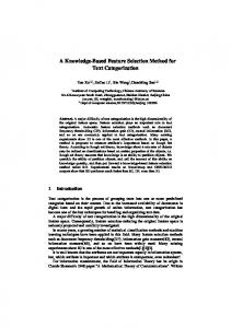
0.025

We assume that the K dimensional feature vectors of the development speakers, originating from a specific phone, can be modeled by an independent, wide sense stationary (WSS), and white Gaussian vector random sequence X[n]. Its covariance function matrix KXX [m, n] can thus be written as, KXX [m, n] = diag(λ1 ...λK )δ[m − n], where λp (p = 1, .., K) are the variances of the individual cepstral coefficients. Now, the Euclidean distance between the mth and nth feature vector will be, 1 2

d(m, n) = ||X[m] − X[n]|| .

d(m, n) = d = ||Z|| ,

0.015

0.01

dth for α = 0.2

0.005

0

Area = 0.1

dth for α = 0.1

0

20

40

(2)

where Z is a zero mean Gaussian random vector having a covariance matrix KZZ found to be, KZZ = diag(2λ1 ...2λK ).

d2 =

Zi2 =

i=1

K 

For simplification, we assume that, the effect of the individual λi values in (3), can be approximated using a lumped param¯ Thus, eter λ. K  ¯ ¯ Wi2 = 2λY, (4) d2 ≈ 2λ i=1

¯ as the average variance given by, where we define λ (5)

K Now, in (4), Y = i=1 Wi2 is a squared sum of zero mean independent Gaussian random variables, and thus will follow a chi-squared distribution given by, (1/2)K (K/2−1) −y/2 e . (6) y Γ(K/2) √ ¯ . Using this transformation in From (4), we have d = 2λY (6), we obtain the PDF of d, given by,  2 21−K/2 dK−2 d fD (d) = ¯ . ¯ K/2 exp − 4λ Γ(K/2) λ fY (y) =

The mean and variance of this distribution can be found as, √ ¯ + K/2) 2 λΓ(1 and (7) μD = Γ(K/2) ¯ − μ2 , respectively. (8) σ 2 = 2K λ D

120

140

160

4.0.2. Calculation of distance threshold In this feature selection problem, we process data on a frameby-frame basis. Assuming that we know the PDF parameters for the current frame, we would select the next frame if its distance from the current frame is greater than a threshold dth . For a fixed value α ∈ [0, 1], we define dth as, P [d > dth ] =

(3)

i=1

K 1  ¯ λi . λ= K i=1

100

Fig. 3. A PDF of inter-feature Euclidean distance and the proposed distance threshold (Shown for α = 0.1 and 0.2).



(2λi )Wi2 , where Wi ∼ N (0, 1).

80

d

Now, from (2), we can write, K 

60

(1)

Since the feature vectors have a common mean, the term inside the parenthesis in (1) will be a zero mean vector random sequence. Also, due to independence assumption, d(m, n) is independent of m and n. Thus, 1 2

0.02

PDF of d

4.0.1. PDF of Euclidean distance between features

D

4496

∞

fD (z)dz = α.

dth

The process is illustrated in Fig. 3 for α = 0.1 and 0.2. This implies that, we select a feature vector only if its distance from the current feature is so high that the event is less probable than α, implying that there must be a change in the phone represented by the feature. We observe that the PDF, fD (d), can be closely approximated by a Gaussian distribution hav2 . Using this approximation, ing a mean μD and variance σD we obtain, √ (9) dth = μD + 2σD erfc−1 (2α), where erfc−1 is the inverse of the complementary error function (erfc). Here, erfc() is defined as:   x 2 2 e−t dt. erfc(x) = π 0 4.0.3. Estimation of PDF parameters We use a recursive method for estimating the feature vector mean and variance similar to [5]. Denoting λ[n] as the vector containing the diagonal elements of KXX [0, 0], and μX [n] as the mean vector of the nth frame, we use the equations, μ ˆ X [n] ˆ λX [n]

= =

βm μ ˆ X [n − 1] + (1 − βm )X[n], and (10) ˆ βv λX [n − 1] + (1 − βv )||X[n] − μ ˆ X [n]||,(11)

where βm , βv ∈ [0, 1) are smoothing parameters.

4.0.4. Implementation Let i denote the current feature index and set j = i + 1. For initialization (i = 1), X[i] is always selected. In this case ˆ X [i] are calculated from X[i] and X[j] as, alone, μ ˆ X [i] and λ μ ˆ X [i] = 0.5(X[i] + X[j]) and ˆ X [i] = 0.5(X[i] ·2 +X[j]·2 ) − μ ˆ X [i]·2 , λ ¯ where ()·2 denotes element-wise square operation. Next, λ, 2 μD , σD and dth are calculated using (5), (7), (8) and (9), respectively. Now, j is iteratively incremented by 1 and d(i, j) ˆ X [i] are upis calculated from (1). The values μ ˆ X [i] and λ dated in each step using (10) and (11), along with dth . If d(i, j) > dth is found, X[j] is selected. Next, i = j and j = i + 1 is set and the process is repeated until the desired number of features are selected. 5. SYSTEM DESCRIPTION Since the objective of this research is focused on the UBM alone, we use a fairly simple GMM-UBM [1] baseline system without any mismatch compensation. For the front-end, 39-dimensional MFCC features (MFCC+Δ+ ΔΔ) was used, followed by feature warping [6] using a 3-s sliding window. To remove silence frames, a phone recognizer based voice activity detector (VAD) was used. For UBM training, 2019 and 2873 utterances from the NIST 2004 1-s data was used, for males and females, respectively. Number of mixtures was set to 1024, since increasing it did not offer further improvement. UBM Training was performed using the maximum likelihood (ML) criterion. For modeling, the gender dependent UBMs were adapted to each enrollment speaker dependent model using classical MAP adaptation [1] with one iteration and a relevance factor of 19. The 5min tel-tel condition trials [3] of the NIST 2008 SRE was used for evaluation. The proposed feature selection algorithm parameters were set experimentally. We used α = 0.1, βm = 0.8, and βv = 0.6 and 0.8, for male and female features, respectively. An alternate set of values may work better with different features or alternate experimental speaker verification setup. The experiments were performed using a high performance cluster computer. 6. RESULTS AND DISCUSSION The EER performance along with the computation time1 required for UBM training using the set of presented approaches is shown in Table 1. Baseline performance with 100% of the data used to train the UBM for male and female trials, is 11.42% and 13.30% EER, respectively. It is clear that all four methods, with 1% of UBM data employed can provide performance equivalent to the baseline system with 1 CPU times calculated were not always precise due to varying load in the cluster computer, which is a shared resource.

4497

Table 1. Comparison of different UBM training schemes with respect to EER and training CPU time. Method

%data

Baseline LFS UFS RFS IFS-EU

100 1 1 1 1

Male EER Time (%) h:mm 11.43 3:46 11.48 0:24 11.54 0:22 11.41 0:18 10.99 0:27

Female EER Time (%) h:mm 13.30 7:36 12.99 0:45 13.13 0:52 13.56 1:25 12.80 1:02

upto 7 times reduced computation time. In addition, using the proposed feature selection scheme, denoted by IFS-EU, we notice a ∼ 0.4% reduction in the EER in comparison to the baseline system for both genders. This is because the selected features in the IFS-EU method are more able to represent the diverse speaker pool, while suppressing some of the fine model traits of intra-speaker phoneme variability, which, we believe, is less important for construction of a UBM. 7. CONCLUSIONS A novel feature frame sub-sampling algorithm for reducing the computational complexity in UBM training was presented and evaluated. Using an inter-feature Euclidean distance based criteria, the proposed method selects feature frames across the speaker acoustic space that are more relevant, and provides improved UBMs with the same or better EER performance compared to conventional UBM training, which employs excessive amounts of data. 8. REFERENCES [1] D. A. Reynolds, T. F. Quatieri, and R. B. Dunn, “Speaker verification using adapted gaussian mixture models,,” Digital Signal Processing, vol. 10, no. 1-3, pp. 19 – 41, 2000. [2] W. Campbell, D. Sturim, D. Reynolds, and A. Solomonoff, “SVM based speaker verification using a GMM supervector kernel and NAP variability compensation,” in in Proc. ICASSP 2006, vol. 1, Toulouse, France, May 2006. [3] “The NIST year 2008 speaker recognition evaluation plan,” 2006. [Online]. Available: http://www.nist.gov [4] C. Barras, X. Zhu, J.-L. Gauvain, and L. Lamel, The CLEAR’06 LIMSI Acoustic Speaker Identification System for CHIL Seminars, ser. Lecture Notes in Computer Science. Springer Berlin / Heidelberg, 2007, vol. 4122. [5] M. M. Bruce, Estimation of variance by a recursive equation. NASA Technical note, 1969. [6] J. Pelecanos and S. Sridharan, “Feature warping for robust speaker verification,” in Proc. 2001: A Speaker Odyssey, 2001, pp. 213–218.