Navigation is a vital issue in the research of Autonomous Mobile Vehicle (AMV). ...... shortest path determined by this algorithm from s3 to g3 is shown in the solid.
Journal of Intelligent and Robotic Systems 32: 361–388, 2001. © 2001 Kluwer Academic Publishers. Printed in the Netherlands.
361
A Novel Navigation Method for Autonomous Mobile Vehicles CANG YE and DANWEI WANG School of Electrical and Electronic Engineering, Nanyang Technological University, Singapore 639798; e-mail: {ecye, edwwang}@ntu.edu.sg (Received: 28 July 2000; in final form: 6 December 2000) Abstract. This paper presents a novel navigation method for Autonomous Mobile Vehicle in unknown environments. The proposed navigator consists of an Obstacle Avoider (OA), a Goal Seeker (GS), a Navigation Supervisor (NS) and an Environment Evaluator (EE). The fuzzy actions inferred by the OA and the GS are weighted by the NS using the local and global environmental information and fused through fuzzy set operation to produce a command action, from which the final crisp action is determined by defuzzification. The EE tunes the supports of the fuzzy sets for the OA and the NS; therefore, the capability of the navigation method is enhanced. Simulation shows that the navigator is able to perform successful navigation task in various unknown or partially known environments, and it has satisfactory ability in tackling moving obstacles. More importantly, it has smooth action and exceptionally good robustness to sensor noise. Key words: behavior control, behavior fusion, fuzzy logic control, obstacle avoidance, path planning, virtual environment.
1. Introduction Navigation is a vital issue in the research of Autonomous Mobile Vehicle (AMV). The navigation of an AMV may be considered as a task of determining a collision free path that enables the AMV to travel through an obstacle course from an initial configuration to a goal configuration, where configuration here refers to the spatial coordinate and the heading angle of the AMV. The process of finding such path is also known as path planning which could be classified into two categories: Global Path Planning and Local Path Planning. Global path planning methods are usually conducted off-line in a completely known environment. Many attempts such as Geometry Algorithm [1, 2], Potential Field Method [3–5] as well as other Heuristic or Approximating Approaches [6–8] for solving this problem have been reported. As a pre-specified environment is required for these methods to plan the path, they fail when the environment is not fully known. On the other hand, the Local Path Planning techniques, also known as the obstacle avoidance methods, are more efficient in AMV navigation in an unknown or partially known environment. It utilizes the on-line sensory information to tackle the uncertainty. Among the proposed methods, Geometry Algorithm assumes that
362
C. YE AND D. WANG
the local obstacles are fully recognized via visual sensor [9, 10] or can be learnt by on-line acquisition via distance sensor [11–13]. The former assumption may not be applicable to a real environment; while in the latter case, it is time consuming to explore an unknown environment. On the other hand, Potential Field Method [14–16] seems more efficient for fast obstacle avoidance as it does not need to know the details of the neighboring obstacles. However, this method has three disadvantages [17]: First, local minimum could occur and cause the AMV to be stuck. Second, it tends to cause unstable motion in the presence of obstacles. Third, it is difficult to find the exact force coefficients influencing the AMV’s velocity and direction in an unknown environment. The practicality of the Potential Field Method therefore hinges on how well these problems can be resolved. In 1985, Brooks [18] introduced the first Behavior Control paradigm. Behavior Control method is based on decomposing the problem of autonomous control by task rather than by function. Traditional function decomposition used a SMPA (Sense-Model-Plan-Act) framework. The SMPA approach [19, 20] consists of modules each of which senses the world, builds a world model, and plans actions for the AMV. It connects the modules in a serial fashion. A serious problem in this approach is reliability. If any module fails, the entire system will break down. Another problem is that it cannot tackle an unknown environment. In contrast, Behavior Control method decomposes the system into special task-specific modules, each of which is connected directly to sensors and actuators and operates in parallel. These modules are generally called Behaviors, and all Behaviors are connected together by an arbitrator to determine the control action of the entire system. A number of methods [21–25] based on Behavior Control have emerged since Brooks introduced the approach. Generally, Behaviors are designed to be relatively simple. Complex tasks are achieved by composing a number of Behaviors to produce an emergent complex Behavior. The composition is accomplished by a Behavior Arbitrator, which resolves any conflicts arising from multiple behaviors attempting to control the same actuator simultaneously. Such architecture at least has four advantages: First, it is able to react in real time due to the parallel operation; Second, it performs well in unknown environment as each Behavior module determines its action in an on-line manner; Third, Behavior modules may be simple and may be easily and flexibly managed; Fourth, it has good robustness, i.e., the system still functions even if one or more of the Behaviors fail. There are two main issues in employing Behavior Control method: Behavior construction and Behavior Fusion. A Behavior module is usually designed to be a Reactive System [21, 22], which maps a perceived situation to an action. Fuzzy Logic Control (FLC) was introduced to construct the Behaviors by numerous researchers [26–29] as FLC requires no mathematical model and is able to represent human expert knowledge on a control plant. To alleviate the burden of constructing a fuzzy controller and maintain the correctness, consistency and completeness of the fuzzy rule base, Neural Network method [25, 33] and Evolutionary algorithm [31] were introduced to construct the fuzzy controller automatically.
A NOVEL NAVIGATION METHOD FOR AUTONOMOUS MOBILE VEHICLES
363
Figure 1. Obstacle avoidance does not know which way is the correct turn [33].
However, it remains to be difficult to seamlessly fuse Behavior components developed independently as there are conflicts among multiple Behaviors when they attempt to control the same actuator simultaneously. Much effort has been devoted to the design of Behavior Fusion method. However, no completely satisfactory solution has yet emerged. Most of the existing Behavior Arbitrators [23–25, 32] adopt the strategy of High-Priority-Take-All. Payton and Rosenblatt [33] identified a serious problem with this priority-based arbitration scheme, which is illustrated by a case of an AMV that encounters an obstacle while it is following a path as shown in Figure 1. In this example, the Path Following Behavior suggests to turn left while the Obstacle Avoidance Behavior suggests to turn either left or right to avoid the obstacle. The priority-based arbitration scheme has one half chance to make the correct turn (left) since the information regarding path following is not available once the arbitrator selects the Obstacle Avoidance Behavior. To resolve this limitation, they developed a command fusion architecture that allows control recommendations from different Behaviors to be directly combined to form multiple control recommendations with different weights, from which a final control command is chosen based on a Winner-Take-All selection strategy. In the Payton–Rosenblatt (P–R) command fusion method, the output of each Behavior is a set of nodes, each of which represents a possible control decision. The desirability of each control decision is represented by the activation level of the node. Figure 2 describes a P–R network for fusing two Behaviors–Turn-ForObstacle and Track-Road-Edges for the situation given in Figure 1. The size and color of each node in Figure 2 represents the Behavior’s activation for that command. The size of a node represents the magnitude of its activation. Solid black color represents positive activation, while white color represents negative activation. For example, the Turn-For-Obstacle Behavior in Figure 2 has a large positive activation level for the “hard left” node, and a large negative activation level for the “straight ahead” node. To fuse these two Behaviors, the activation strengths of the corresponding nodes are combined using a weighted sum scheme, as illustrated in Figure 2. The weight associated with a Behavior reflects the degree of importance of its command recommendation. For instance, the Turn-For-Obstacle has a higher
364
C. YE AND D. WANG
Figure 2. Payton–Rosenblatt network for fusing turn command for two behaviors [33].
weight than the Track-Road-Edges Behavior because it is more important to avoid hitting obstacles than to follow the track. The final control command is the node with the largest positive activation in the combined Behavior based on the WinnerTake-All selection strategy. In the case illustrated in Figure 2, the final control command is to turn “hard left”. Langer and Rosenblatt [34] applied a similar architecture to off-road navigation to arbitrate the commands from the Behaviors of Avoid-Obstacle, Road-Following, Goal-Seeking, Maintain-Heading and Path-Tracking. Yen and Pfluger [35] (Y–P) extended Payton and Rosenblatt’s work by using Fuzzy Logic. Their command arbitrator fused the Allowed Direction recommended by Fuzzy-Obstacle-Avoidance Behavior and Fuzzy-Path-Following Behavior to determine the final control command. A problem remaining in these two command fusion methods is that the weight for each Behavior is constant. But actually the desirability of each Behavior may vary from situation to situation. For example, the weight of Turn-For-Obstacle Behavior may be larger in the case that an obstacle is lying in the middle of the path, and it may be smaller if the obstacle is only slightly obstructing the path. This means that the weights of Behaviors shall be subjected to environmental information in order to obtain a better fusion of the Behaviors. Y–P and P–R command fusion methods fail to do so. To overcome the disadvantages of the above-mentioned methods, we propose a new Behavior Fusion method in this paper. It employs FLC to weight the Behaviors using both local and global environmental information and fuses the fuzzy command actions recommended by each Behavior. Based on this Behavior Fusion method, we proposed a new navigator for the navigation of AMV in a floor space. It consists of an Obstacle Avoider (OA), a Goal Seeker (GS), a Navigation Supervisor (NS) and an Environment Evaluator (EE). The fuzzy actions inferred by the OA and the GS are weighted by the NS and fused through fuzzy set operation to produce a command action, from which the final crisp action is determined by defuzzification. This paper is organized as follows: In Section 2, the vehicle model, the navigation task and the overall architecture of the fuzzy navigator are described. In Section 3, the Goal Seeker (GS) is introduced and its function is verified by sim-
A NOVEL NAVIGATION METHOD FOR AUTONOMOUS MOBILE VEHICLES
365
ulation. In Section 4, the Navigation Supervisor (NS) which fuses the obstacle avoidance behavior and the goal seeking behavior is presented. In Section 5, the function of the EE is briefed. In Section 6, the navigator’s ability is extended to an indoor floor space. In Section 7, the performance of the navigator is analyzed in a virtual indoor environment. Finally, the paper is concluded in Section 8.
2. Overview of the Navigator 2.1. VEHICLE MODEL As we intend to develop a platform independent navigation method, the assumption we make regarding the platform is only that the AMV is able to steer its heading direction by synchronous drives and can detect obstacles by its distant sensors. This places no particular shape or size on the AMV. However, for the convenience of simulation, we use a cylindrical AMV model with a radius of Rv and assume there are N distant sensors evenly distributed along a ring. The value of N is upper bound by the beam angle of the distant sensor such that no cross talk is caused due to beam overlap. In this study, we assume that the AMV’s radius to be 20 cm and there are 24 ultrasonic sensors arranged in a ring. Each sensor, si for i = 1, 2, . . . , 24, gives a distance to the obstacle, li , in its field of view, where 4 cm � li � 400 cm, and each sensor covers an angular view of 15◦ . For obstacle detection and avoidance purposes, the sensors in the front of the AMV is divided into five sensor groups (sgi for i = 1, . . . , 5) as depicted in Figure 3, which give the AMV a view angle of 225◦ . The five sensor groups are denoted as sgi , for i = 1, . . . , 5, where each group is composed of 3 neighboring sensors.
Figure 3. Diagram of the AMV and the arrangement of the distance sensors.
366
C. YE AND D. WANG
Figure 4. Diagram of the coordinate system and the control variables.
With this sensor arrangement, the distance, di , measured by the ith sensor group from the center of the AMV to the obstacle is expressed as: di = Rv + min(lj | j = 3i − 2, 3i − 1, 3i);
for i = 1, . . . , 5.
(1)
The remaining sensors are used to detect the obstacle distance along the goal direction for Behavior Fusion. The reason for arranging the sensors into groups is that: (1) it reduces input dimension, hence reduces the complexity of the navigation method; and (2) it reduces the possibility of misdetection of obstacles.
2.2. COORDINATE SYSTEM AND NAVIGATION TASK The coordinate systems and the control variables of the AMV are depicted in Figure 4. The two coordinate systems are the world coordinate denoted by XOY, and the AMV coordinate given by xoy. A navigation task is defined as to navigate the AMV from a start configuration to its goal coordinate without colliding with the obstacles in between. Each navigation task is specified in the world coordinate. The AMV configuration is represented by S = (Xo , Yo , θ)T , where Xo and Yo is the coordinate of the AMV’s center, and θ stands for the heading angle of the AMV. Without considering the AMV’s dynamics, we assume that the control variables are its linear velocity, v, and the change in the heading angle, �θ, which is referred as steering angle hereafter. Suppose a navigation task from a start configuration s to a goal coordinate g is specified as in Figure 5. It can be achieved through an iterative process as follows: (1) At time step t, t = 0, 1, . . . , k, . . ., acquire the environment information, di and Pg (Xg , Yg ), and the AMV’s configuration S(t) = (Xo (t), Yo (t), θ(t))T ;
A NOVEL NAVIGATION METHOD FOR AUTONOMOUS MOBILE VEHICLES
367
Figure 5. Process of achieving a navigation task.
(2) Determine the output variables v(t + 1) and θ(t + 1), where θ(t + 1) = θ(t) + �θ(t); then update the AMV’s configuration by the following equation: θ(t + 1) S(t + 1) = Xo (t + 1) Yo (t + 1) θ(t) + �θ(t) = Xo (t) + v(t + 1)�T cos(θ(t) + �θ(t)) , Yo (t) + v(t + 1)�T sin(θ(t) + �θ(t))
(2)
where �T is the time interval between two time steps. (3) Iterate this situation-action mapping process (step 1 and 2) until the goal is achieved. 2.3. ARCHITECTURE OF THE NAVIGATOR The architecture of the proposed navigator is depicted in Figure 6. It consists of four main modules: an Obstacle Avoider (OA), a Goal Seeker (GS), a Navigation Supervisor (NS) and an Environment Evaluator (EE). Fuzzy Logic is used to construct the OA, GS and NS. The function of OA is to determine the action for avoiding the obstacle encountered without considering if it will cause deviation from the goal. The input variables are di for i = 1, . . . , 5, where di are the sensor readings; and W is the variable determining the fuzzy sets for the input space. The value of W is determined by the EE. For a specific value of W , the sensor readings, di are fuzzified and encoded into the fire strength of the j th rule, then the fuzzy inference is made and the fuzzy control action, Va and ��a , are given. The function of the GS is to infer the action for goal seeking without considering obstacle avoidance. The input variables of this module are dg and φ, where dg is the
368
C. YE AND D. WANG
Figure 6. Diagram of the proposed navigator. The input variables of each module is referred to Figure 4.
magnitude of the goal vector pg (xg , yg ), and φ is the angle between the goal vector and y axis. The input variables are fuzzified, then the fuzzy inference is made and the fuzzy control action, Vg and ��g , are given. The role of the NS is to fuse the actions of the OA and the GS in order to perform collision-free navigation. It consists of three sections: the Behavior Weighting Section (BWS), the Behavior Fusing Section (BFS) and the State Evaluation Section (SES). The input variables of the BWS are dog and dmin , where dog is the distance of the obstacle locating along the goal vector pg (xg , yg ), and dmin = min(di ) is the minimum value of the five sensor readings. These two variables are fuzzified based on the fuzzy sets determined by W for the input space, and the fuzzy inference is made. Finally, the Behavior coefficient τ is given by defuzzification. The Behavior Fusion is implemented in the BFS. The actions inferred by the OA and GS are weighted by (1 − τ ) and τ , respectively, and are fused to produce the fuzzy command action, V and ��. Finally, the crisp control action of the AMV is given by defuzzification. Each Behavior module is developed independently. To construct the GS module, the OA is simply ignored (τ = 1) such that V = Vg and �� = ��g meaning the Defuzzification Section in the BFS could be merged into the GS to form a complete fuzzy controller. The OA is constructed similarly. The method of constructing the OA is referred to [30] where Yung and Ye introduced a reinforcement learning method to learn the fuzzy rule base automatically. This paper will describe the construction of the GS and propose a new method for Behavior Fusion.
A NOVEL NAVIGATION METHOD FOR AUTONOMOUS MOBILE VEHICLES
369
As can be seen from this Behavior Control navigation method, the OA utilizes the local environmental information – di to infer a local action to avoid the neighboring obstacles; while the GS uses the global environmental information – pg (xg , yg ) to determine a global action to move towards the goal. The NS keep a balance between these two actions by weighting them based on a local and a global environmental information, dmin and dog , respectively. Through this Behavior Fusion scheme, the local and global navigation targets – avoiding obstacles and achieving the goal are achieved. 3. Goal Seeker The input variables of this controller are dg and φ, and the control outputs are vg and �θg (the Defuzzification Section of the BFS is merged into the GS in this case, therefore, we denote the output by vg and �θg ), respectively. As depicted in Figure 4, the goal vector with respect to the AMV’s coordinate can be calculated by pg (xg , yg ) = Pg (Xg , Yg ) − Po (Xo , Yo ).
(3)
The magnitude of this vector and the deviation of the AMV’s heading direction are denoted by dg = |pg (xg , yg )|,
(4)
φ = θ − ψ,
(5)
and
where ψ is the angle between the relative goal vector pg (xg , yg ) and the horizontal axes, and is given by � � −1 yg . (6) ψ = tan xg The membership functions of these four variables are shown in Figure 7. As the velocity inferred by the OA is upper bound by 16 cm/s [30], Vg max is also set to 16 cm/s for consistency. In accordance with the membership functions of the input variables, the rule base consists of 28 rules, each of which is denoted by Rj : IF φ is !j AND dg is Dj THEN vg is Vj , �θg is ��j ; for j = 1, . . . , 28, where Rj denotes the j th rule; !j is the fuzzy set for φ in the universe of discourse Uφ ⊂ R in the j th rule, which takes the linguistic value of NB, NM, NS, ZZ, PS, PM, or PB; Dj is the fuzzy set for dg in the universe of discourse Udg ⊂ R in the j th rule and takes the value of VN, NR, FR or VFR; while Vj is the fuzzy set for vg in the universe of discourse Uvg ⊂ R, each of which takes the value of VS, SL, FS,
370
C. YE AND D. WANG
Figure 7. Membership functions of the input/output variables for the GS. VN: very near; NR: near; FR: far; VFR: very far; VS: very slow; SL: slow; FS: fast; VF: very fast; NB: negative big; NM: negative middle; NS: negative small; ZZ: zero; PS: positive small; PM: positive middle; PB: positive big; Vg max : maximum value for this behavior. Table I. Fuzzy rules for the GS dg
φ
VN NR FR VFR
NB
NM
NS
(VS,PB) (VS,PB) (SL,PB) (SL,PB)
(VS,PM) (VS,PM) (SL,PM) (FS,PM)
ZZ
PS
(VS,PS) (VS,ZZ) (VS,NS) (SL,PS) (SL,ZZ) (SL,NS) (FS,PS) (FS,ZZ) (FS,NS) (VF,PS) (VF,ZZ) (VF,NS) Control Action (vg , �θg )
PM
PB
(VS,NM) (VS,NM) (SL,NM) (FS,NM)
(VS,NB) (VS,NB) (SL,NB) (SL,NB)
or VF, and ��j is the fuzzy set for �θg in the universe of discourse U�θg ⊂ R, each of which takes the value of NB, NM, NS, ZZ, PS, PM, or PB. These rules are constructed and tuned through human expert knowledge and given in Table I. Taking the first rule for an example, it is read as: IF φ is NB and dg is VN THEN vg is VS and �θg is PB. As Rj can be represented as a fuzzy relation, Rj : !j × Dj → {Vj , ��j }, the rule base can be represented as the union � R = � =
28 �
Rj
� =
j =1 28 � j =1
28 �
[!j × Dj → Vj , !j × Dj → ��j ]
j =1
RVj ,
28 � j =1
R�j
(7) = {RV , R�},
A NOVEL NAVIGATION METHOD FOR AUTONOMOUS MOBILE VEHICLES
371
where R consists of sub-rule-bases, RV and R�, associated with the control actions, vg and �θg , respectively. Each sub-rule-base consists of 28 rules. The j th rules, RVj and R�j are fuzzy relations in the product space, Uφ × Udg × Uvg and Uφ × Udg × U�θg respectively. Thus, the rules can be implemented as fuzzy relations with the corresponding membership functions. The membership value of the j th rule, RVj and R�j , are denoted by µRVj (φ, dg , vg ) and µR�j (φ, dg , �θg ), respectively. For the input φ = φ � and dg = dg� , which can be treated as fuzzy singleton � φ = !� and dg� = D � in the universe of discourse Uφ and Udg , the fuzzy control actions, V � and ��� are inferred by Zadeh’s compositional rule of inference [20]. They are given by �
�
�
V = (! , D ) ◦
28 �
RVj
and
�
�
�
�� = (! , D ) ◦
j =1
28 �
R�j ,
(8)
j =1
where ◦ denotes the maximum minimum operation. If mamdani’s minimum operation is applied to the fuzzy relations, the membership values of V � and ��� are calculated by µV � (vg ) =
28 �
µj (φ � , dg� ) ∧ µVj (vg )
and
j =1
µ��� (�θg ) =
28 �
(9) µj (φ
�
, dg� )
∧ µ��j (�θg ),
j =1
where µj (φ � , dg� ) is the fire strength of the j th rule for the inputs φ = φ � and dg = dg� , which is given by µj (φ � , dg� ) = µ!j (φ � ) ∧ µDj (dg� ).
(10)
A defuzzification process is required to determine the crisp output actions, vg and �θg , from the fuzzy control action, Vg and ��g . For the reason of limiting the computing cost, we adopted the method of height defuzzification here. The crisp control action is given by
28
28 � � � � j =1 µj (φ , dg )pj j =1 µj (φ , dg )qj and �θg = 28 , (11) vg = 28 � � � � j =1 µj (φ , dg ) j =1 µj (φ , dg ) where pj is the center of fuzzy set Vj ; and qj is the center of fuzzy set ��j . For the membership functions defined for vg and �θg , pj takes a crisp value of 0, Vg max /2, 3Vg max /4 or Vg max, while qj takes a value of −π/4, −π/6 −π/12, 0, π/12, π/6 or π/4. After the construction of the GS, its goal seeking function is verified by simulation as illustrated in Figure 8. Given three start configurations with different
372
C. YE AND D. WANG
Figure 8. Verification of the GS from three start points to a goal.
locations and different heading directions and a goal location, the AMV turned to the goal direction and moved toward the goal. When it was approaching the goal, it reduced its velocity gradually and finally stopped at the goal location. 4. Navigation Supervisor Since the OA and the GS work independently, their individual results of v and �θ have to be fused together in order to make navigation sense. The original Navigation Supervisor (NS) performing this role was proposed in [32] which use the IF-THEN rules to switch between obstacle avoidance and goal seeking Behavior. For a smoother and better Behavior transient, a new NS based on fuzzy control is proposed. It consists of three sections: the BWS, the BFS and the SES. 4.1. BEHAVIOR WEIGHTING SECTION The BWS is a fuzzy controller which takes dmin and dog as the input and infer the Behavior coefficient τ . Here, dmin stands for the minimum value of the sensor readings and is given by dmin = min(di | i = 1, 2, . . . , 5),
(12)
and dog represents the minimum distance to the obstacle located along the relative goal vector pg (xg , yg ). In order to detect this distance value, a sensor group is dynamically configured (depicted in Figure 9) as si for i = k − 1, k, k + 1, where k is calculated from the deviation of the AMV’s heading direction φ. The sensor along the y axis is numbered by 8, and the index number of the sensors is counted down clockwise, therefore, we have � � 12φ , (13) k = 8 − int π where φ is determined by Equation (5) and int(•) refers to the rounding to the nearest integer. If i is zero or negative, the modulo-24 of i is used instead. The distance, dog detected by the sensor group is given by dog = Rv + min(li | i = k − 1, k, k + 1).
(14)
A NOVEL NAVIGATION METHOD FOR AUTONOMOUS MOBILE VEHICLES
373
Figure 9. Configuration of the dynamic sensor group.
Figure 10. Membership functions of the input/output variables for the BWS. VN: very near; NR: near; FR: far; VS: very small; SM: small; BG: big; VB: very big. Table II. Fuzzy rules for the BWS dmin
dog VN NR FR
VN
NR
FR
VS SM SM
SM SM BG τ
SM BG VB
The membership functions of the input and output variables are depicted in Figure 10. The membership functions of the input variables take exactly the same form as the OA [30], where Rv = 20 cm and W determining the support of each fuzzy set is tuned by the EE. In accordance with the membership functions of the input variables, the rule base of the NS consists of nine rules only. They are given in Table II. At each time step, the input variables are fuzzified and the fuzzy inference is made. Finally, the crisp value of the Behavior coefficient, τ , is determined by
374
C. YE AND D. WANG
defuzzification. As the process of constructing the BWS is similar to the GS, we omit it for conciseness.
4.2. BEHAVIOR FUSING SECTION The implementation of the Behavior Fusion is depicted in Figure 11. As shown in Figure 11(a), the fuzzy sets of the steering angle inferred by the OA and the GS, ��a and ��g , are weighted by (1 − τ ) and τ respectively, and yield ���a and ���g . Then ���a and ���g are aggregated to yield fuzzy set ��. In the same way, the fuzzy sets of the velocity, Vg and Va , are fused to produce fuzzy set V as depicted in Figure 11(b). To infer the crisp command action of the AMV, a defuzzification process is required. We employ the method of height defuzzification for simplicity and the result is given by
v=
τ
243 � � � j =1 µj (φ , dg )pj + (1 − τ ) m=1 µm (d )b1m
28
� τ j =1 µj (φ � , dg� ) + (1 − τ ) 243 m=1 µm (d )
28
and �θ =
τ
(15a)
243 � � � j =1 µj (φ , dg )qj + (1 − τ ) m=1 µm (d )b2m ,
28
� τ j =1 µj (φ � , dg� ) + (1 − τ ) 243 m=1 µm (d )
28
(15b)
where µm (d � ) is the fire strength of the mth rule of the OA for the input d � = (d1� , d2� , d3� , d4� , d5� ), while b1m and b2m are the centers of the mth fuzzy sets for va and �θa [30].
(a) Figure 11. Behavior fusion of the navigator.
(b)
A NOVEL NAVIGATION METHOD FOR AUTONOMOUS MOBILE VEHICLES
375
4.3. STATE EVALUATION SECTION
A State Evaluator inside the NS is employed to correctly guide the AMV in the case that the goal is located very near to an obstacle. Its control flow is as follows: Firstly, if the condition, dg < dog is satisfied, then dog is set as dog = Rv + ls max , where ls max stands for the maximum detectable distance of the ultrasonic sensor. This may result in a large value of τ , hence, a large portion of goal seeking behavior since the goal is visible in this case. Secondly in the case that µVN (dmin ) < µVN (dog ), µVN (dog ) > 0.5 and dg < dog are satisfied, the fuzzy inference is prohibited, i.e., τ is set to 1 because the goal is visible and is very near the obstacle. To verify the smoothness of the Behavior transition of the NS, three typical cases are simulated and the Behavior coefficient versus the navigation time step is depicted in Figure 12. In each case, the Behavior coefficient decreases/increases gradually when encountering/leaving the obstacle. Therefore, the NS transits the obstacle avoidance and goal seeking Behaviors gradually instead of switches between them. The distinct benefit of this Behavior Fusion scheme is that it may result in a smooth motion.
Figure 12. Behavior transition in various obstacle cases (W = 40 cm).
376
C. YE AND D. WANG
Figure 13. Performance of the Environment Evaluator. Table III. Value of W given by the EE 28 cm < dmin � 68 cm 68 cm < dmin � 88 cm 88 cm < dmin � 148 cm dmin > 148 cm W = 20 cm W = 30 cm W = 60 cm W = 80 cm
5. Environment Evaluator Usually, a navigator with the OA, GS and NS modules should be able to perform the desired navigation task. One problem with such a navigator is that it could be ‘near-sighted’. For instance, in the case illustrated in Figure 13, a reasonable action would be to turn left. However, as the navigator is ‘near-sighted’ with a small value of W = 20 cm [30], it fails to deal with the obstacle on its right side, therefore it continues its path towards the obstacle then turns right and follows the boundary of the obstacle instead. The purpose of the Environment Evaluator (EE) is to equip the navigator with a more balanced near-sightedness and far-sightedness. Principally, the EE tunes the fuzzy sets of the input variables for the OA and the NS adaptively by adjusting the value of W based on the variables dmin . The scheme employed here is show in Table III. The performance of the EE was evaluated and the results are illustrated in Figure 13. As can be seen, the AMV turned left and moved smoothly toward its goal location with the aid of the EE. In addition, the EE enabled the AMV to keep a larger clearance from the obstacle, by allowing it to navigate a longer distance. In addition, the EE is very useful for navigating the AMV in a floor space where the obstacle density may vary from rooms to rooms. The AMV may use a large value of W to tackle a sparse obstacle course keeping a large clearance with the obstacles in one room; while it may use a small value of W enabling it to go into a crowded obstacle course in another room. The performance of the proposed navigator with the EE was verified from different start configurations to different goals in various unknown environments. Figure 14 depicts some difficult cases where the goals are hided by the obstacles
A NOVEL NAVIGATION METHOD FOR AUTONOMOUS MOBILE VEHICLES
377
Figure 14. Navigation in an unknown environment.
Figure 15. Flow chart of the navigation in the whole floor space. C – A threshold to represent a sub-goal achieved; s – Start configuration; E – Permitted position error for the goal achieved; g – Goal position.
or the goals are located very near the obstacles. The AMV is able to navigate successfully to the goals in all cases. 6. Navigation in a Virtual Indoor Environment For future application in real world navigation, the proposed navigator is integrated with a Virtual Environment (VE) simulator [36] which is able to render the top view and 3D visualization of the VE (Figure 18) in real time. The performance of the navigator is studied in the VE which is a floor plan as depicted Figure 16. In order to navigate the AMV from one room to another room in such a large floor space, a path planner based on the A∗ Algorithm [37] is used to extract a shortest path via
378
C. YE AND D. WANG
Figure 16. Navigation in the whole floor space.
Figure 17. Comparison with the DistBug method.
(a)
(b)
Figure 18. Navigation from s3 to g3 in the DIP Lab: (a) Top view of the DIP Lab; (b) 3D camera view at point p1 .
A NOVEL NAVIGATION METHOD FOR AUTONOMOUS MOBILE VEHICLES
379
a set of sub-goals, sg1 , . . . , sgj , . . ., from the coordinates of the corners and the doors which are assumed to be known. Then the start configuration, the sub-goals and the goal are queued and represented by P1 , . . . , Pi , . . . , which is fetched one by one to the navigator. The flow chart of this scheme is depicted Figure 15. When Pi is a sub-goal, dg is set to any value that satisfies dg � 12Rv to prevent the GS from reducing the AMV’s velocity as referring to the fuzzy rules listed in Table I. The navigation scheme is verified by simulation to be able to navigate the AMV in the floor space. Figure 16 depicts the navigation task from s1 to g1 and s2 to g2 respectively. 7. Performance Comparison with Related Methods In this section we compare our Behavior Fusion method with the related methods and study their performances. As mentioned before, the proposed Behavior Fusion method utilizes Fuzzy Logic Control. In this respect, it is similar to Y–P’s command fusion algorithm [35]. A difference is that our method uses the environmental information to weight each Behavior while Y–P’s algorithm combines the command recommendation from each Behavior directly. This difference may result in different navigation performance. Kamon and Rivlin [38] proposed a new navigation algorithm called DistBug, which could be considered as an extension of Lumelsky’s [39] Bug algorithm. They proposed a new leaving condition allowing the AMV to abandon boundary following Behavior as soon as global convergence is guaranteed. Our proposed method shares the following identical features with the DistBug algorithm: (1) employs two reactive Behaviors – goal seeking and obstacle avoidance; (2) utilizes the global information – the obstacle distance along the goal vector to arbitrate between Behaviors. The different features are: (1) DistBug is a priority-based arbitrator, while our method uses fuzzy logic to fuse the Behaviors. Hence, Behavior transits gradually from one to another instead of being switched between them. Therefore, the motion is smooth when the AMV encounters an obstacle or leaves the obstacle. (2) Our proposed method uses one more local parameters, dmin , to fuse the Behaviors, this is more reasonable as the AMV has to consider the nearest obstacle even if the goal becomes visible. (3) DistBug assumes a point AMV (without considering its kinematic and dynamic constraints) such that the AMV turns abruptly at both the hit point (H1 for both paths, B1 and B2 , planned by the DistBug method as depicted in Figure 17) and the leaving points (L1 and L2 ), or at the corners (e.g., C1 and C2 ) of the obstacle while following its boundary. Our proposed navigation algorithm takes into account of the kinematic constraints in developing the GS, the OA and the NS, therefore, this disadvantage is overcome.
380
C. YE AND D. WANG
7.1. SMOOTHNESS OF MOTION The DIP Lab, as depicted in Figure 18, of the floor space is used for performance study. Taking the navigation from s3 to g3 for an instance, the acceleration is within (−9.5 cm/s2 , 9.5 cm/s2 ) and the angular acceleration is within (−0.70 rad/s2 , 0.41 rad/s2 ) during the entire navigation meaning there is no abrupt change in both the velocity and the angular velocity. Considering the Nomad XR400 mobile robot with a maximum translation acceleration of 5 m/s2 and a maximum rotational acceleration of 2 rad/s2 , the motion of our navigator is quite smooth and may be easily controlled. This property has an obvious benefit for practical application when the AMV’s dynamics become an important consideration.
7.2. QUALITY OF THE NAVIGATED PATH To evaluate the path achieved by the navigator, the Visibility Graph Method is used to determine the shortest path for each navigation task. For instance, the shortest path determined by this algorithm from s3 to g3 is shown in the solid line in Figure 18. At each time step, the deviation of the AMV’s position from the shortest path is denoted by dae . The length of the actual path and the shortest path are represented by pa and pe , respectively, and the relative error between the actual path length and the shortest path length, (pa − pe )/pe is denoted by Er . Based on the floor plan of the DIP lab, six navigation tasks were conducted and the results are tabulated in Table IV. It can be seen that: (1) the navigator achieves a path reasonably close to the shortest path; (2) the less obstacles the AMV has to tackle, the shortest the path is; (3) the relative error and the path deviation are proportional to the number of obstacles. For the first point, the largest relative error is only 5.7% for Task 1, whereas the smallest error is 1.2% when there is no obstacle. For the second point, we can see that the relative error decreases as the number of obstacles decreases. For the third point, the trend is clear that the navigated path will deviate a lot more from the shortest path if there are more obstacles present in the environment. Table IV. Navigation under various obstacle courses Task
Pa /cm
pe /cm
Er
Avg. dae
Max. dae
Time
No. of obstacle
1 2 3 4 5 6
830.4 791.0 680.7 583.8 492.9 424.1
785.6 759.8 660.1 573.0 485.0 422.9
5.7% 4.1% 3.1% 1.9% 1.6% 1.2%
14.4cm 9.3cm 7.3cm 4.0cm 3.5cm 3.1cm
39.5cm 33.1cm 28.0cm 12.8cm 9.6cm 8.2cm
73.4s 69.8s 61.8s 54.2s 49.1s 45.6s
7 6 5 4 2 0
A NOVEL NAVIGATION METHOD FOR AUTONOMOUS MOBILE VEHICLES
381
7.3. CAPABILITY OF DEALING WITH MOVING OBSTACLE The proposed navigator works in an on-line manner and does not need a priori knowledge of the environment. The command action of the navigator is determined based on the on-line sensor readings. Therefore, it may be capable of dealing with moving obstacle. To test this particular capability, three case studies were simulated. In these three case studies, the AMV was specified the same navigation task from a start to a goal. In the first case as depicted in Figure 19, the AMV was to navigate from the bottom to the top of the space, while the obstacle was approaching the AMV at a constant velocity from the left. If the AMV continues its trajectory at maximum velocity (16/cm) ignoring the presence of the obstacle, it would have collided with the obstacle at point p. However, the AMV has ability for obstacle avoidance, which enables it to steer away to avoid the obstacle. In the simulation scene depicted in Figure 19(a), it can be seen that the AMV slowly turned right as it detected the presence of the obstacle. Figure 19(b) renders the scenario after the AMV has successfully avoided the obstacle and moved to its goal. Simulations on varying the obstacle’s velocity show that collision occurred when the velocity of the obstacle is greater than 6cm/s (38% of the AMV’s maximum velocity). What this means is that as long as the obstacle is moving at a reasonably low speed, the navigator is capable of avoiding it. In the second case as depicted in Figure 20, using the same start and goal configurations, the obstacle is heading directly towards the AMV at a constant velocity. This is the worst case for the AMV to avoid obstacle in fact because of the relative velocity is the sum of both. Figure 20(a) depicts the AMV turned left to avoid the obstacle; and Figure 20(b) renders the scenario just after the AMV
(a) Figure 19. Avoiding a dynamic obstacle from the left.
(b)
382
C. YE AND D. WANG
(a)
(b)
Figure 20. Avoiding a dynamic obstacle heading towards the AMV.
(a)
(b)
Figure 21. Overtaking a dynamic obstacle.
has successfully avoided the obstacle and moved to its goal. Further simulations on varying the obstacle’s velocity show that collisions occur when the velocity of the obstacle is greater than 3 cm/s (19% of the AMV’s maximum velocity). As can be seen, the navigator’s avoidance capability is relatively lower because of the higher relative velocity. In the third case as depicted in Figure 21, the AMV is to overtake an obstacle moving with a constant velocity along the same direction. It is assumed that the AMV’s velocity is higher. Figure 21(a) depicts the AMV turned left and began to overtake the obstacle; and Figure 21(b) renders the scenario after the AMV has successfully overtaken the obstacle and moved to its goal. Further simulations on
A NOVEL NAVIGATION METHOD FOR AUTONOMOUS MOBILE VEHICLES
383
varying the obstacle’s velocity show that collisions occur when the velocity of the obstacle is greater than 7 cm/s (44% of the AMV’s maximum velocity). In summary, the navigator is capable of tackling simple moving obstacle course as long as the velocity is upper bounded. 7.4. ROBUSTNESS TO NOISY SENSOR READING The robustness to noisy sensor reading is quite important for a navigator. For a real AMV, sensor readings are often noisy, especially in the case that coarse sensors such as ultrasonic sensor are used. The noise of the sensor may cause incorrect obstacle distances and further cause error in navigation. In the worst case, the noise of the sensor may cause collision. Therefore, a navigation algorithm shall have a large tolerance to noisy sensor data. Due to the limitations of physical experimentation, such as high cost, unrepeatability and damage in the case of collision, simulation is an essential and efficient measure to test the robustness of a navigation algorithm. It is also an efficient platform for tuning the navigation algorithm in order to improve its robustness in the development stage. Taking into consideration the navigation task from s3 to g3 , as depicted in Figure 18, we tested the robustness of our proposed navigator in the presence of various degrees of sensor noise. For comparison purpose, the same simulation conditions as Yen and Pfluger [35] was used. The simulated sensor noise is assumed to have a uniform probability distribution in the interval [−d × n, d × n] where d is the actual distance, and n is the sensor noise rate which has 7 different value, 0, 0.1, 0.2, 0.4, 0.6, 0.8 and 1.0, in this simulation. The AMV performed the navigation task 100 times in each sensor noise rate. For measuring the robustness, we adopt the following definitions as the same as [35]: DEFINITION 1 (Safety Index (SI)). c¯ – the percentage of the simulation runs in which the AMV successfully reaches the goal without collision.
DEFINITION 2 (Steering Smoothness Index (SSI)). ω¯ = ki=1 |�θ¯i |/k, where �θ¯i stands for the absolute average steering angle in the ith simulation run.
DEFINITION 3 (Velocity Smoothness Index (VSI)). a¯ = ki=1 |�v¯i |/k, where �v¯i stands for the absolute average of the velocity change in the ith simulation run. The result of the empirical evaluation is summarized in Table V and plotted in Figure 22, which shows a degradation of the Safety Index and Smoothness Index of the proposed navigator as the amount of sensor noise increases. For the Smoothness Index, the SSI increases only 1.54 times larger while the VSI increases 4.45 times larger, meaning VSI is more sensitive to the sensor noise. As the maximum value of SSI is equivalent to 4.3◦ , the degradation of SSI is graceful. The maximum value of VSI is 1.58 cm/s, which is relatively large compared with the maximum velocity
384
C. YE AND D. WANG
Table V. Robustness to sensor noise Sensor noise rate
SSI (rad)
VSI (cm/s)
SI
0.00 0.10 0.20 0.40 0.60 0.80 1.00
0.0297 0.0304 0.0360 0.0428 0.0513 0.0655 0.0753
0.29 0.35 0.45 0.62 0.83 1.34 1.58
1.00 1.00 1.00 0.98 0.97 0.95 0.94
Figure 22. Smoothness and safety vs. noise rate.
of the AMV – 16 cm/s. However, this result is not unexpected as the sensor is very noisy. Even if the sensor noise rate is as high as 100 percent, the navigator is still able to tackle the obstacle course in most cases. The result means that the navigator has high robustness to noisy sensor data. Therefore, it has high practicality to real AMV navigation, in which sensor noise cannot be ignored. For a comparison with Yen and Pfluger’s command fusion method, their result is cited and tabulated in Table VI. As these two sets of data are from different simulations, the comparison of absolute values should carry no significance. But the Relative Degrade of the Steering Smoothness Index (RDSSI) and the Relative Degrade of the Safety Index (RDSI) with reference to the case of 0 sensor noise rate are comparable and could be used to compare our navigator with the Yen and Pfluger’s (YP’s) navigator. The results are shown in Table VII, and the comparison between the RDSSIs and the RDSIs are depicted in Figure 23. We can observe that: (1) both the RDSSI and RDSI of our navigator and YP’s navigator increase with sensor noise, meaning that both smoothness of the steering and safety degrade over sensor noise; (2) the RDSSI of YP’s navigator increases faster than our navigator (best case was about 13 times faster and worst case was 84 times faster), which means that YP’s navigator is more sensitive to sensor noise than our navigator;
A NOVEL NAVIGATION METHOD FOR AUTONOMOUS MOBILE VEHICLES
385
Table VI. Robustness to sensor noise for YP’s navigator Sensor noise rate
SSI (rad/s)
SI
0.00 0.10 0.20 0.40 0.60 0.80 1.00
0.137 0.408 0.820 1.559 2.146 2.683 3.075
1.00 1.00 0.989 0.978 0.933 0.944 0.911
Table VII. Comparison of our navigator with YP’s navigator Sensor noise rate
0.10 0.20 0.40 0.60 0.80 1.00
RDSSI
RDSI
Proposed
YP’s
Proposed
YP’s
2.36% 21.21% 44.11% 72.73% 120.54% 153.54%
197.8% 498.5% 1038.0% 1466.4% 1858.4% 2144.5%
0% 0% 2% 3% 5% 6%
0 1.1% 2.2% 6.7% 5.6% 8.9%
(3) the RDSSI of our navigator with noise rate of 1.0 is still less than that of YP’s navigator with noise rate of 0.1, which means that our navigator is much more robust to sensor noise; (4) the RDSI of our navigator is smaller than that of YP’s navigator in the same noise rate.
8. Conclusions We have presented a novel navigation method for the navigation of AMV in unknown environments. It employs Fuzzy Logic Control and utilizes local and global environmental information to weight the obstacle avoidance and goal seeking Behaviors, the control actions recommended by these two Behaviors are fused to produce a final command action, from which the crisp control action of the AMV is determined through defuzzification. Due to the nature of Behavior Control architecture, the proposed navigation method is able to tackle unknown and dynamic environment. As Behavior transits gradually from one to the other by using Fuzzy Logic Control, the overall control action is smooth than the Bug family methods.
386
C. YE AND D. WANG
Figure 23. Comparison of the robustness of our navigator with YP’s navigator.
Furthermore, the navigation method has exceptionally good robustness to sensor noise. Acknowledgement Part of the work presented in this paper was completed when the first author was studying for his Ph.D. degree in the Department of Electrical and Electronic Engineering, the University of Hong Kong. The financial support from the department and the technical guidance from Dr. Nelson Yung are appreciated. The contribution of F. P. Fong on the 3D simulator is also acknowledged. References 1. 2.
3. 4. 5.
Mitchell, J. S. B.: An algorithm approach to some problems in terrain navigation, Artificial Intelligence 37 (1988), 171–201. Janét, J. A., Luo, R. C., and Kay, M. G.: Autonomous mobile robot motion planning and geometric beacon collection using traversability vector, IEEE Trans. Robotics Automat. 13(1) (1997), 132–140. Khatib, O.: Real-time obstacle avoidance for manipulators and mobile robots, Internat. J. Robotics Res. 5(1) (1986), 90–98. Hwang, Y. K. and Ahuja, N.: A potential field approach to path planning, IEEE Trans. Robotics Automat. 8(1) (1992), 23–32. Guldner, J. and Utkin, V. I.: Sliding mode control for gradient tracking and robot navigation using artificial potential fields, IEEE Trans. Robotics Automat. 11(2) (1995), 247–254.
A NOVEL NAVIGATION METHOD FOR AUTONOMOUS MOBILE VEHICLES
6. 7. 8. 9. 10. 11. 12.
13.
14. 15. 16. 17.
18. 19. 20. 21.
22.
23.
24. 25. 26. 27.
387
Brooks, R. A.: Solving the find-path problem by good representation of free space, IEEE Trans. Systems Man Cybernet. 13(3) (1983), 190–197. Brooks, R. A.: Planning collision-free motions for pick-and-place operations, Internat. J. Robotics Res. 2(4) (1983), 19–40. Lozano-Perez, T.: Spatial planning: A configuration space approach, IEEE Trans. Comput. 32(2) (1983), 108–120. Feng, D. and Krogh, B. H.: Satisficing feedback strategies for local navigation of autonomous mobile robots, IEEE Trans. Systems Man Cybernet. 20(6) (1990), 1383–1395. Rao, N. S. V.: Robot navigation in unknown generalized polygonal terrains using vision sensors, IEEE Trans. Systems Man Cybernet. 25(6) (1995), 947–962. Lumelsky, V. J., Mukhopadhyay, S., and Sun, K.: Dynamic path planning in sensor-based terrain acquisition, IEEE Trans. Robotics Automat. 6(4) (1990), 530–540. Oommen, B. J., Iyengar, S. S., et al.: Robot navigation in unknown terrains using learned visibility graphs. Part I: The disjoint convex obstacle case, IEEE J. Robotics Automat. 3(6) (1987), 672–681. Rao, N. A. V. and Iyengar, S. S.: Autonomous robot navigation in unknown terrains: incidental learning and environment exploration, IEEE Trans. Systems Man Cybernet. 20(6) (1990), 1443–1449. Borestein, J. and Koren, Y.: Real-time obstacle avoidance for fast mobile robot, IEEE Trans. Systems Man Cybernet. 19(5) (1989), 1179–1186. Borestein, J. and Koren, Y.: The vector field histogram – fast obstacle avoidance for mobile robots, IEEE J. Robotics Automat. 7(3) (1991), 278–288. Chung, J. H. and Ahuja, N.: An analytical tractable potential field model of free space and its application in obstacle avoidance, IEEE Trans. Systems Man Cybernet. 28(5) (1998), 729–736. Koren, Y. and Borenstein, J.: Potential field methods and their inherent limitations for mobile robot navigation, in: Proceedings of the 1991 IEEE International Conference on Robotics and Automation, Sacramento, CA, April 1991, pp. 1398–1404. Brooks, R. A.: A robust layered control system for a mobile robot, IEEE J. Robotics Automat. 2(1) (1986), 14–23. Thorpe, C., Hebert, M., et al.: Vision and navigation for the Carnegie–Mellon navlab, IEEE Trans. Pattern Anal. Mach. Intell. 10(3) (1988), 362–373. Barshan, B. and Durrant-Whyte, H. G.: Inertial navigation systems for mobile robots, IEEE Trans. Robotics Automat. 11(3) (1995) 328–342. Arkins, R. C.: Motor schema based navigation for a mobile robot: An approach to programming by behavior, in: Proceedings of the IEEE International Conference on Robotics and Automation, 1987, pp. 264–271. Schoppers, M. J.: Universal plans for reactive robots in unpredictable environments, in: Proceedings of the Tenth International Joint Conference on Artificial Intelligence, 1987, pp. 1039–1046. Kweon, S., Kuno, Y., Watanabe, M., and Onoguchi, K.: Behavior-based intelligent robot in dynamic indoor environment, in: Proceedings of IEEE/RSJ International Conference on Intelligent Robots and Systems, 1992, pp. 1339–1346. Gat, E., Desai, R., et al.: Behavior control for exploration of planetary surfaces, IEEE Trans. Robotics Automat. 10(4) (1994), 490–503. Beom, H. R. and Cho, H. S.: A sensor-based navigation for a mobile robot using fuzzy logic and reinforcement learning, IEEE Trans. Systems Man Cybernt. 25(3) (1995), 464–477. Sugeno, M. and Nishida, M.: Fuzzy control of a model car, Fuzzy Sets and Systems 16 (1985), 103–113. Pin, F. G. and Watanabe, Y.: Using fuzzy behaviors for the outdoor navigation of a car with low-resolution sensors, in: Proceedings of IEEE/RSJ International Conference on Intelligent Robotics and Systems, 1993, pp. 548–553.
388 28.
29. 30. 31. 32.
33. 34. 35.
36.
37. 38. 39.
C. YE AND D. WANG
Tunstel, E.: Coordination of distributed fuzzy behaviors in mobile robot control, in: Proceedings of IEEE International Conference on Systems, Man, and Cybernetics, 1995, pp. 4009– 4014. Gerke, M. and Hoyer, H.: Fuzzy collision avoidance for industrial robot, in: Proceedings of IEEE/RSJ International Conference on Intelligent Robots and Systems, 1992, pp. 510–517. Yung, N. H. C. and Ye, C.: An intelligent mobile vehicle navigator based on fuzzy logic and reinforcement learning, IEEE Trans. Systems Man Cybernet. 29(2) (1999), 314–321. Seng, T. L., Khalid, M. B., and Yusof, R.: Tuning a neuro-fuzzy controller by genetic algorithm, IEEE Trans. Systems Man Cybernet. 29(2) (1999), 226–236. Yung, N. H. C. and Ye, C.: An intelligent navigator for mobile vehicles, in: Proceedings of the International Conference on Neural Information Processing, Hong Kong, September 24–27, 1996, pp. 948–953. Payton, D. W., Rosenblatt, J. K., and Keirsey, D. M.: Plan guided reaction, IEEE Trans. Systems Man Cybernet. 20(6) (1990), 1370–1382. Langer, D., Rosenblatt, J. K., and Hebert, M.: A behavior-based system for off-road navigation, IEEE Trans. Robotics Automat. 10(6) (1994), 976–983. Yen, J. and Pfluger, N.: A fuzzy logic based extension to Payton and Rosenblatt’s command fusion method for mobile robot navigation, IEEE Trans. Systems Man Cybernet. 25(6) (1995), 971–978. Yung, N. H. C. and Ye, C.: EXPECTATIONS – An autonomous mobile vehicle simulator, in: Proceedings of IEEE International Conference on Systems, Man and Cybernetics, Orlando, Florida, October 12–15, 1997, pp. 2290–2295. Latombe, J. C.: Robot Motion Planning, Kluwer Acad. Publ., Dordrecht, 1991. Kamon, I. and Rivlin, E.: Sensory-based motion planning with global proof, IEEE Trans. Robotics Automat. 13(6) (1997), 814–822. Lumelsky, V. J. and Stepanov, A. A.: Path-planning strategies for a point mobile automaton moving admist obstacles of arbitrary shape, Algorithmica 2 (1987), 403–430.