x4. 1. 3. ) x2. 1 + x1x2 + (â4+4x2. 2)x2. 2. (12). The Six Hump Camel function is defined in two ..... ceedings of the IEEE Conference on Systems, Man and Cybernetics, pp. ... [10] Kennedy, J.: Small Worlds and Mega-Minds: Effects of Neighbor-.
A novel particle swarm niching technique based on extensive vector operations I.L. Schoeman and A.P. Engelbrecht
Abstract Several techniques have been proposed to extend the particle swarm optimization (PSO) paradigm so that multiple optima can be located and maintained within a convoluted search space. A significant number of these implementations are subswarm-based, that is, portions of the swarm are optimized separately. Niches are formed to contain these subswarms, a process that often requires user-specified parameters. The vector-based PSO uses a novel approach to locate and maintain niches by using additional vector operations to determine niche boundaries. As the standard PSO uses weighted vector combinations to update particle positions and velocities, the proposed technique builds upon existing knowledge of the particle swarm. Once niche boundaries are calculated, the swarm can be organized into subswarms without prior knowledge of the number of niches and their corresponding niche radii. This paper presents the vector-based PSO with emphasis on its underlying principles. Results for a number of functions with different characteristics are reported and discussed. The performance of the vector-based PSO is also compared to two other niching techniques for particle swarm optimization.
1
Introduction
Swarm intelligence algorithms such as Particle Swarm Optimization (PSO) have been proved to be effective and robust for difficult optimization problems where the more traditional optimization methods would not succeed [6] [9] [22] [23]. PSO was specifically designed to face the challenge of optimizing problems described by convoluted problem landscapes, often characterized by many sub-optimal or near-optimal solutions. The two-fold nature of the PSO algorithm that balances a social and a cognitive component facilitates both the exploitation of regions with higher fitness, as well as the exploration of the entire problem space. In both these aspects the velocity term, which is also a unique PSO feature, plays a significant role [13]. The concept of velocity is part of the metaphor of a swarm of particles flying through and exploring hyperdimensional space. Particles move towards the target and overshoot it, but being pulled back by previous successes, oscillate around the target before eventually converging on the best solution [16] [26]. If, in 1
the process of exploration, better fitness is encountered, the direction of the entire swarm changes and it is pulled away from a suboptimal solution. If a problem is such that the locations of multiple optima are required, it is expected that different regions of the search space, known as niches, should be optimized in order to locate the different optima. Therefore, algorithms must be designed that counteract the effect of one of the essential characteristics of the particle swarm, namely redirecting the swarm away from a suboptimal solution to a better solution. Different strategies have been devised to neutralize this effect and maintain an optimal solution once it has been located, for example, by modification of the objective function [17] [18], using the cognition-only PSO at certain stages of the algorithm [4] [5], and setting a niche radius to contain particles in a niche [1] [14]. Algorithms implementing these strategies, are known as niching or speciation algorithms. The remainder of this paper is organized as follows: Section 2 gives an overview of niching algorithms, while section 3 discusses the underlying principles of the vector-based niching approach and describes the vectorbased PSO. Section 4 reports and discusses experimental results. Section 5 presents a comparative study of three niching algorithms, while section 6 concludes the paper.
2
PSO niching algorithms
The idea of optimizing portions of a swarm separately has been implemented in a variety of PSO algorithms, mainly to improve diversity [6] [10] [11] [12]. Topological neighbourhoods are formed in different ways by selecting particles using their indices. The particles constituting such a subswarm are distributed throughout the search space. Most of these neighbourhoods or subswarms will eventually converge, but premature convergence is prevented, ensuring a better chance to locate a good solution. The notions of subswarms and neighbourhoods form a natural starting point when designing niching algorithms. For such strategies neighbourhoods are spatial, not topological. A neighbourhood can be conceptualized as the region in search space where the problem landscape is such that each particle has a natural tendency to move towards an optimum or neighbourhood best. The particles in such a region constitutes a subswarm. A number of niching algorithms is described below. Not all use the idea of neighbourhoods explicitly, but in each case a strategy is implemented to optimize candidate solutions separately. Objective function stretching: A function stretching technique proposed by Parsopoulos et al was originally devised to overcome the problem of occasional convergence to local optima [17]. Parsopoulos and Vrahatis [18] also used this principle to locate all the local minima of a function sequentially.
2
The objective function is modified to prevent the PSO from returning to a previously discovered minimum. All local minima above the current minimum are eliminated. Each time a minimum is discovered, the function is modified and the swarm re-initialized. However, the stretching technique introduces false local minima as well as misleading gradients [24]. nBest PSO: Brits et al developed a particle swarm optimization algorithm, the nbest PSO, to solve systems of unconstrained equations [3]. Systems with multiple solutions require the implementation of a niching strategy, and the standard gbest algorithm is adapted to locate multiple solutions in one run of the algorithm. For a system with two variables x and y, each particle represents a set of candidate values for x and y. The fitness function is formulated to indicate the distance between curves described by the equations, which is minimized to find a solution. NichePSO: This strategy, developed by Brits et al [4] [5], creates subswarms from particles representing candidate solutions and each particle’s closest topological neighbour. Candidate solutions are identified by monitoring the fitness of a particle over a number of iterations, selecting those where the fitness changes very little. These initial subswarms absorb particles from the main swarm (the remaining particles after subswarms have been formed) or merge with other subswarms while being optimized in parallel, until the main swarm contains no more particles. Main swarm particles are updated using the cognitive-only PSO, while subswarms are updated separately, using the Guaranteed Convergence Particle Swarm Optimization (GCPSO) algorithm [25]. The Speciation-Based PSO: The speciation-based PSO (SPSO) of Bird and Li [1] and Li [14], is an elegant niching approach where particles are first sorted according to their fitnesses. Niches are then formed, starting with the fittest particle, by incorporating all particles within a previously set niche radius in the subswarm that is formed in the niche. The process is repeated until no more particles remain. Particles are updated once, using their respective neighbourhood best positions. The entire process is repeated until stopping conditions are met. Disadvantages of such an approach is the need to set a niche radius in advance. Even if an optimal value for the niche radius is estimated, performance will degrade for function landscapes with different niche sizes. The adaptive niching PSO: Bird and Li [1] proposed the adaptive niching PSO (ANPSO) that removes the need to specify the niche radius in advance. The average distance between each particle and its closest neighbour is calculated and organized in an undirected graph. At each iteration, an edge is added to the graph between every pair of particles that have been closer than the average distance to one another during the last 2 steps. Niches are formed from these connected subgraphs while all unconnected particles remain outside any niches. Thus the neighbourhood topology is redefined at every step. Particles are updated in each niche, while those outside any 3
niche will continue searching the whole problem space. The algorithm performed well on a number of benchmark functions but is computationally expensive, owing to the calculation of distances between particles. The Fitness Euclidian-distance ration PSO: Li [15] proposed a multimodal particle swarm optimizer based on fitness Euclidian-distance ratio (FER-PSO) to remove the need for niching parameters. The FER-PSO uses a memory-swarm that contains all personal bests, in order to keep track of the multiple better points found so far. Each of these points are further improved by moving toward its “fittest and closest” neighbours, identified by computing a particle’s FER value. The FER value is a ratio of the difference in fitness of two particles and the Euclidian distance between them, scaled by a factor to ensure that neither the fitness nor the distance becomes too dominant. The effect of such a strategy is that particles would form niches naturally around multiple optima, given that there are sufficient numbers of particles. The Waves of Swarm Particles algorithm: The Waves of Swarm Particles (WoSP) algorithm, developed by Hendtlass [7], uses a technique to alter the behaviour of PSO so that further aggressive exploration is achieved after each optimum has been explored. A short-range force (SRF) is introduced that produces a force of attraction between particles that is inversely proportional to the distance between them. As particles approach each other, their velocity increases significantly. Some particles may pass each other and move apart until the short-term attraction is too weak to bring them back together. Particles will not be pulled back, but continue moving rapidly apart, exploring beyond their previous positions. Instead of converging on a single optimum, some of the neighbourhood will be ejected with significant velocities, thus exploring other regions of the search space. Such particles are organized in a wave, and particles assigned to the wave are attracted to the best particle in the wave. The wave converges on another optimum, starting the process again until all or most of the optima are located.
3
The vector-based PSO
The vector-based PSO, developed by Schoeman and Engelbrecht [19] [20] [21], comprises a novel approach to niching where, instead of suppressing certain characteristics of the particle swarm optimization paradigm, the power of the concepts underlying the original PSO is harnessed to induce niching. In addition, the strategy has the ability to locate and optimize multiple optima with minimal prior knowledge of the landscape of the objective function. The number of control parameters is minimal, while care is taken to retain a robust and accurate algorithm that will yield good performances for a variety of problem landscapes. Three versions of the vector-based PSO were developed, all using the
4
same strategy to identify niches and calculate niche radii, but differing in the optimization phase. The sequential vector-based PSO [19] locates a niche and optimizes the subswarm occupying it sequentially. Duplicate solutions are found, which makes the approach clumsy, especially as the dimensionality increases. The parallel vector-based PSO [20] identifies niches sequentially, but optimizes them in parallel, merging niches that converge on the same optimum in the process. The enhanced parallel vector-based PSO [21] incorporates an additional strategy to prevent particles from leaving a niche, preventing possible redirection of the swarm and loss of optimal solutions. In this article the enhanced parallel vector-based PSO, now referred to as the vector-based PSO is presented, as it represents the culmination of the strategy.
3.1
Using vector properties
Vectors are used extensively in PSO algorithms. Concepts such as the tendency to move towards the personal best as well as the global best are implemented using vectors, as is the concept of a velocity associated with a particle. These vectors are manipulated to locate a new position. If these vectors could also be manipulated to facilitate niching, the resulting strategy would be elegant as well as powerful. During optimization of a swarm of particles, the velocity vector associated with a particle is updated as follows: vi,j = wvi,j + c1 r1,j (yi,j − xi,j ) + c2 r2,j (ˆ yj − xi,j )
(1)
where w is the inertia weight [22] , c1 and c2 two positive acceleration constants and r1,j and r2,j random values between 0 and 1. In the updating equation, vector addition is used to add weighted position vectors towards a particle’s personal best position and towards the best position found so far in the entire neighbourhood. The resulting vector is added to the previous velocity weighted by w. The new velocity is used to compute a new particle position. In the following paragraphs a strategy is explained that uses vector properties and operations to locate niche boundaries. Consider the inverted one-dimensional Rastrigin function: F (x) = −(x2 − 10 cos(2πx) + 10)
(2)
where x ∈ [−1.5, 1.5]. Figure 1 illustrates the function with three optima in this range. Let the initial best position be at x = 0. The neighbourhood comprises the entire search space, therefore this position is known as yˆ or gbest. Assume that a number of particles are distributed along the x-axis. Each particle has an associated personal best position (yi or pbest) where the fitness will be better than at the original particle position. Positions of two 5
Figure 1: The inverted one-dimensional Rastrigin function, showing particles with associated vectors particles are shown with vectors pointing in the direction of the personal best position as well as towards the global best position. If a particle is in a region where particles are expected to converge on the current neighbourhood best position, vectors towards the particle’s personal best position as well as the neighbourhood best position point in the same direction. If the vectors point in opposite directions, it means that the position of the particle is in a region where it is not expected to converge on the current neighbourhood best position. When identifying niches, this knowledge can be used to identify particles that are not in the niche surrounding the current neighbourhood best position. Not all particles where both vectors point in the same direction will, of course, move towards the neighbourhood best position, as there may be other optimal solutions between those particles and the current neighbourhood best. To illustrate vectors in a two-dimensional search space, Figure 2 shows a contour map of the two-dimensional Ursem F1 function: F (x1 , x2 ) = −(sin(2x1 − 0.5π) + 3cos(x2 ) + 0.5x1 )
(3)
Two particles, P 1 and P 2, are depicted with their associated vectors vp and vg where gbest is a position at or near to the global optimum of the function. During optimization, vector addition of the position vectors towards a
6
Figure 2: Contour map of the two-dimensional Ursem F1 function particle’s personal best and current neighbourhood best positions is used to update the velocity vector. These vectors are implemented as arrays of values of which the size corresponds to the dimensionality of the problem. In the vector-based PSO, the niching strategy uses another vector operation, the dot product. The dot product of a and b is computed as follows: a · b = a1 b1 + a2 b2 + a3 b3
(4)
The angle between two nonzero vectors a and b is defined to be the angle θ where θ ∈ [0, π]. The relationship between the dot product and the angle between two vectors is described by: a · b = kakkbk cos θ
(5)
The value of cos θ is positive in the first quadrant θ ∈ [0, π/2] and negative in the second quadrant θ ∈ [π/2, π]. Therefore the dot product of two vectors is positive if they point roughly in the same direction, that is, with an angle of less than 90◦ between them. The dot product is negative when the vectors point roughly in opposite directions, that is, with an angle between 90◦ and 180◦ between them. For one-dimensional functions, the angle is either 0◦ or 180◦ . These observations illustrate that a position in the search space can be calculated that roughly indicates the boundary between two niches, using the existing vectors vp and vg . The position where the dot product changes from positive to negative indicates the approximate niche boundary. 7
3.2
Identifying niches
Two steps are needed to locate multiple optimal solutions. Firstly, candidate solutions are identified and portions of the search space - called a niche where an optimal solution may be found are demarcated. Secondly, each subswarm is optimized while particles are contained in the niche. The vector-based PSO uses the vector dot-product to compute the distance from each neighbourhood best to the boundary of that niche, known as the niche radius. A number of niching algorithms use the concept of a niche radius, although niche boundaries can, at best, be approximated. Handled with care, a niche radius indicates an approximate region containing particles belonging to the niche. The vector-based PSO identifies niches sequentially and calculates a niche radius for each candidate solution. Algorithm 1 presents a pseudo-code description of the process. Some aspects of the algorithm are discussed in detail below: Algorithm 1 Process to identify niches begin Initialize the swarm by creating N particles; Set niche identification number (niche-id )of each particle to 0 ; for each particle do Create a random position within a small radius �; The position with the best fitness is the personal best yi (t); The other position is xi (t) ; Calculate the vector vpi , where vpi (t) = yi (t) − xi (t) end repeat Set y ˆ(t) to yi (t) with best fitness of particles where niche-id = 0; for each particle in the swarm do Calculate the vector vgi where vgi (t) = y ˆ(t) − xi (t) Calculate the dot product δi : δi = vpi · vgi Set radius ρi to the distance between y ˆ(t) and xi (t) end Set niche radius to distance between y ˆ(t) and nearest particle with δi < 0; for each particle where ρi < nicheradius and δi > 0 do Set niche-id to next number; end until no particles with niche-id = 0 remain; if particles in niche < 3 then Create extra particles in niche so that it has at least 3 particles; end
end
8
Initialize the swarm: A specified number of particles is created at random positions throughout the search space. To locate all the optima in the search space, it is essential that particles are distributed uniformly throughout the search space. In this study results are presented using Sobol sequences, one of the most popular quasi-random or low-discrepancy sequences [2], [8], to calculates initial particle positions. During initialization, the personal best position of each particle is calculated. A random position is created in the vicinity of the particle position. A parameter, �, a small value relative to the search space, acts as an upper bound to the distance between the particle position and its personal best position. The position with the best fitness becomes the personal best position and vice versa. Identify niches: The particle with the best fitness of its personal best position is identified as the first neighbourhood best, y ˆ(t). For every particle in the entire swarm, the position vector from the particle’s position to the current neighbourhood best position, vgi , is calculated, as well as the dot product, δi , of the vectors vgi and vpi . The niche radius is set to the Euclidian distance between the current neighbourhood best position and the position of the nearest particle with a negative dot product. Particles with positive dot products and radii smaller than the niche radius constitute a subswarm that can be optimized separately. The process is repeated until all particles have been incorporated in subswarms. False niches: The shape of a niche in an unknown function landscape can not be assumed to be symmetrical around a position identified as the current neighbourhood best. In addition, an initial candidate solution will not be situated at the center of such a niche. Thus the niche radius only gives a rough estimate of the boundary of the niche. However, a number of particles belonging to the niche, may still be situated outside the niche radius, especially if the niche has an irregular shape. In such cases extra or false niches form next to the niche where the true optimum will eventually be located; the particle identified as its neighbourhood best being the particle nearest to that niche. Extending subswarms: Some of the subswarms formed when niches are identified may contain very few particles. Often only one particle constitutes a subswarm with y ˆ(t) equal to yi (t). Such a particle easily becomes stationary and will not converge, or converge very slowly to the nearest optimal solution. False niches are especially prone to such conditions. To prevent subswarms from becoming stationary, more particles are added to these niches. The VBPSO extends subswarms to contain at least 3 particles, a number arrived at through careful empirical observations.
9
3.3
Optimizing and merging subswarms
Once all niches have been identified, subswarms contained in the niches are optimized in parallel. Niches are merged if the distance between two candidate solutions becomes less than a specific problem-dependent threshold value, referred to as the granularity (g). The merging procedure is invoked at specific intervals during the optimization process. Particles are absorbed by the niche with the fittest neighbourhood best. To prevent too many niches merging, particles are not absorbed at the same time; the neighbourhood best being the last to be absorbed. The merging procedure is formalized in algorithm 2. Algorithm 2 The merging procedure begin for each niche do for all other niches do Calculate Euclidian distance between y ˆ(t) of two niches; If distance < granularity for all particles in subswarm with worst y ˆ(t) fitness do Calculate Euclidian distance to y ˆ(t) of other niche; if distance < granularity and particle 6= y ˆ(t) then Set niche-id of particle to that of niche with best fitness; Update number of particles in both niches; end if one particle y ˆ(t) remains and distance < g then Set niche-id of particle to that of niche with best fitness; Update number of particles in both niches; end end
end end end Experiments have shown that the vector-based PSO locates optima successfully for a range of granularity values, where the upper bound for such values is the smallest interniche distance in the problem landscape. During optimization, particles have to be contained in the niche. A particle may move outside the niche, encounter better fitness and redirect the entire subswarm to a neighbouring niche. A strategy has been introduced to counteract this effect. During updating of particle positions, each potential new position is investigated to determine whether the new position is still inside the niche. A particle position is only updated if the vector dot-product remains positive. 10
Algorithm 3 presents a pseudo-code description of the complete vectorbased PSO algorithm. The updating process is repeated for a specified number of times, interspersed with the merging procedure that is called after a set number of iterations. Algorithm 3 The vector-based PSO begin Initialize the swarm by creating N particles; Set (niche-id ) of each particle to 0 and initialize granularity g ; Identify niches and calculate niche radii; Extend each subswarm to contain at least 3 particles; for m times do for k times do for each particle do Create temporary particle xtemp (t) and personal best ytemp (t) ; Calculate vectors vpt emp , vgt emp and dot product δtemp ; if δtemp < 0 then Retain original particle position and corresponding values; end else Particle position xi (t) = xtemp (t); Update yi (t), y ˆ(t) and vectors vpi and vgi ; Update dot product δi and radius ρi ; end end end Merge niches; end
end
4
Experimental results
The performance of the vector-based PSO was tested extensively on a number of functions. Seven two-dimensional functions with a variety of landscapes were chosen to assess the ability of the vector-based PSO to locate optima with differing shapes, sizes and spacing. Short descriptions of each function are listed. Figures 3 to 9 illustrate the function landscapes of the functions for the search space where they have been tested, as well as in a larger space when applicable.
11
The modified Himmelblau function: F (x1 , x2 ) = 200 − (x21 + x2 − 11)2 − (x1 + x22 − 7)2
(6)
The Himmelblau function, defined in two dimensions, has four well-defined optima with similar fitnesses. The function was tested in the range x1 , x2 ∈ [−6, 6], where the optima occur. The Rastrigin function: ! n X � 2 � F (x) = − xi − 10 cos(2πxi ) + 10
(7)
i=1
The function has a global optimum at [0, 0]n where n indicates the number of dimensions, as well as an infinite number of optima radiating out from the global optimum. The Rastrigin function was tested in the range x1 , x2 ∈ [−1.25, 1.25], where the two-dimensional version has 9 optima. The Griewank function: n
F (x) = −
1 X 2 xi 4000
! −
i=1
n Y
! ! xi cos( √ ) + 1 i i=1
(8)
The Griewank function also has one global optimum at [0, 0]n , and an infinite number of optima of which the fitness decrease, depending on the distance from the global optimum. The Griewank function was tested in the range x1 , x2 ∈ [−5.0, 5.0] where the function has 5 optima. The Ackley function: r −0.2
F (x1 , x2 ) = 20 + e − 20.e
2 x2 1 +x2 2
−e
cos(2πx1 )+cos(2πx2 ) 2
(9)
The function has an infinite number of optima surrounding a central global optimum. Fitnesses of the surrounding optima decrease sharply. The function was tested in the range x1 , x2 ∈ [−1.6, 1.6] where 9 optima occur. The Ursem F1 function: F (x1 , x2 ) = −(sin(2x1 − 0.5π) + 3cos(x2 ) + 0.5x1 )
(10)
The function has a repetitive character but no central optimum. Welldefined optima occur indefinitely. The Ursem F1 function is tested in the range x1 ∈ [−2.5, 3.0] and x2 ∈ [−2.0, 2.0], a region containing two of the optima. 12
The Ursem F3 function: �
� � � 2 − |x2 | 3 − |x1 | F (x1 , x2 ) = − (sin(2.2πx1 − 0.5x1 )) · · 2 2 � � � � � 2 − |x1 | 2 − |x2 | · − sin(0.5πx22 + 0.5π) · 2 2 (11) The landscape of the function contains a number of flattened peaks. Groups of four peaks are repeated at specific intervals. The algorithms are tested with one such group in the range x1 , x2 ∈ [−2.0, 2.0]. The Six Hump Camel function: � � x4 F (x1 , x2 ) = 4 − 2.1x21 + 1 x21 + x1 x2 + (−4 + 4x22 )x22 3
(12)
The Six Hump Camel function is defined in two dimensions and is not repetitive. The range x1 ∈ [1.1, 1.1] and x2 ∈ [−1.9, 1.9] contains the six optima and the function is tested in this region.
4.1
Experimental procedure
A number of additional settings is required: Number of initial particles: Initial swarm sizes are chosen arbitrarily, taking into account the dimensions of the search space, the dimensionality and the expected number of solutions. Particle positions are calculated using Sobol sequences [2] [8]. The number of particles chosen for each function is listed in table 1. The granularity: Taking into account the dimensions of the search space, granularity values for each function are chosen, and listed in table 1.
Figure 3: The Himmelblau function showing maxima.
13
(a)
(b) Figure 4: The Rastrigin function.
(a)
(b) Figure 5: The Griewank function.
(a)
(b) Figure 6: The Ackley function.
14
(a)
(b)
Figure 7: The Ursem F1 function.
(a)
(b)
Figure 8: The Ursem F3 function.
Figure 9: The six hump camel function.
15
Number of runs: For all functions, the algorithm is run 30 times and averages of the outcomes calculated. Number of iterations: During the optimization phase, 500 iterations of the updating procedure take place. Niches are merged at intervals of 50 iterations, giving rise to larger subswarms. The intervals are chosen arbitrarily and no evidence could be found that it has any effect on performance. Number of function evaluations: For each function the average number of function evaluations over 30 runs is reported. Due to the extension of small subswarms, the number of function evaluations differ for each run.
4.2
Results
Results of testing the vector-based PSO algorithm with seven two-dimensional functions are reported in table 1. Some aspects of the reported results are clarified in the following description: Average number of solutions: The number of optima located during each run of the algorithm is averaged over 30 runs. Average derivatives: Deviations from the optimal positions are obtained by calculating partial derivatives f 0 (x1 ) and f 0 (x2 ). of the functions. Averages of the derivatives over 30 runs are reported. Success rate: The success rate is the total number of optima located over 30 runs as a percentage of the total number of possible optima. Standard deviation: The standard deviation, placed in parentheses below each average, was calculated for all results.
4.3
Discussion
The results reported in table 1 show that the vector-based PSO performed well on a number of two-dimensional functions with varying function landscapes. The average success rate for all seven functions is 99.71% , and the success rate for individual functions are above 99% in all cases. Function landscapes of the Ackley, Ursem F3 and Six hump camel functions show asymmetrical niche shapes and heights that may differ considerably, but results are still good. Therefore it can be concluded that the vector-based PSO is a robust niching algorithm that performs well even in adverse circumstances.
16
17 60
30
40
50
Ackley
Ursem F1
Ursem F3
Six hump camel
40
Griewank
60
30
Himmelblau
Rastrigin
Particles
Functions
0.3
0.3
0.5
0.3
0.1
0.5
0.5
Granularity
43114 (3952)
39348 (4299)
25686 (4107)
51329 (5062)
50322 (5204)
31850 (4132)
25292 (3759)
Average ] evaluations (Std Dev)
5.97 (0.18)
4 (0)
2 (0)
8.97 (0.18)
8.97 (0.18)
5 (0)
4 (0)
Average ] solutions (Std Dev)
2.41425E-06 (1.96445E-06)
0.510012 (0.275055)
1.26567E-06 (4.9825E-07)
0.232341 (0.710507)
9.56233E-05 (6.79309E-05)
2.10892E-06 (1.05604E-06)
1.86633E-05 (1.6102E-05)
Average f 0 (x1 ) (Std Dev)
6.40035E-06 (2.5426E-06)
0.760007 (0.275063)
0 (0)
0.171993 (0.553919)
9.56233E-05 (6.79309E-05)
1.79454E-06 (8.9928E-07)
1.56231E-05 (1.46347E-05)
Average f 0 (x2 ) (Std Dev)
Table 1: Experimental results using Sobol sequences as a random number generator
99.4444%
100%
100%
99.6296%
99.6296%
100%
100%
Success rate
5
Scalability of the vector-based PSO
A study of a niching algorithm would not be complete without investigating its ability to scale to massively multi-modal domains. Of the functions tested thus far, the Griewank and Rastrigin functions can be singled out as suitable for testing scalability. In addition, the absolute Sine function is a good choice as it easy to visualize its representation in several dimensions.
(a)
(b)
Figure 10: The absolute Sine function in one and two dimensions
5.1
Experimental procedure
This section presents empirical results obtained when testing the vectorbased PSO algorithm on three multimodal functions; the absolute Sine function and the Rastrigin function for 1 to 4 dimensions and the Griewank function for 1 to 3 dimensions. Function landscapes of the two-dimensional Rastrigin and Griewank functions are illustrated in Figures 4 and 5. The absolute Sine function was investigated in the range [0, 2π]n where 1 ≤ n ≤ 4 and is illustrated for one and two dimensions in Figure 10. For each function the algorithm is run 30 times for each of the dimensions. In all cases Sobol sequences are used to compute the initial particle positions.
5.2
Results
Table 2 presents the results obtained for the three functions as described above. For each function in every one of the dimensions, the total number of optima, swarm size used, average number of evaluations over 30 runs and the success rate are reported.
5.3
Discussion
Results show that the vector-based PSO performs well when scaled to higher dimensions, even if swarm sizes are not increased exponentially for higher dimensions.
18
19
Optima 2 4 8 16 3 9 27 81 3 7 23
Dimensions 1 2 3 4 1 2 3 4 1 2 3
Function
Absolute Sine
Rastrigin
Griewank
20 50 150
20 50 150 250
10 40 100 200
Swarm size
4503 19033 67626
10738 48611 154268 291669
5781 13407 98524 223436
Evaluations
Table 2: Scalability results for three functions
98.8889% 99.5238% 99.5652%
100% 99.2593% 99.2593% 88.8889%
100% 100% 100% 100%
Success rate
6
A comparative study of three niching algorithms
Various niching methods for particle swarm optimization have been described in section 2. This section compares the performance of two of those methods, the species-based PSO and NichePSO, to that of the vector-based particle swarm optimizer. In all three niching methods optimization of subswarms takes place in parallel, but the manner in which niches form, differs as explained in section 2.
6.1
Experimental procedure
Comparison of different algorithms requires similar experimental setups. The species-based PSO and NichePSO algorithms are tested on the same seven two-dimensional functions as the vector-based PSO, using the same number of particles for each function. Given that the initial distribution of particles throughout the problem space can influence the performance of an algorithm considerably, both the species-based PSO and the vector-based PSO were implemented using Sobol sequences as a random number generator. NichePSO uses Faure sequences, that also yields an even distribution. The number of iterations was also set to 500 for each algorithm. Average results of 30 runs were calculated for each algorithm. The species-based PSO requires a niche radius set in advance. Each function was tested with a small range of niche radii. Results using the radius yielding the best outcomes are reported. NichePSO was tested using the CILib framework developed by the CIRG research group at the department of Computer Science, University of Pretoria (http://cilib.sourceforge.net). NichePSO requires a merging parameter, µ. For each function, µ was set to the granularity used in the vector-based algorithm, but it was normalized as required by NichePSO.
6.2
Results
Results are reported in table 3. The success rate of each algorithm for each function is reported. In order to compare the algorithms, results of the vector-based PSO are repeated in the table. The granularity, niche radius or merging parameter is listed for every function, as well as the number of particles.
20
21
] Particles
30 40 60 60 30 40 50
Functions
Himmelblau Griewank Rastrigin Ackley Ursem F1 Ursem F3 Six hump camel
0.5 0.5 0.1 0.3 0.5 0.3 0.3
100% 100% 99.6296% 99.6296% 100% 100% 99.4444%
Vector-based PSO Granularity Success rate 3.75 3 0.6 0.6 1.8 0.7 0.6
99.1667% 100% 91.1111% 78.5185% 86.6667% 73.3333% 63.8889%
Species-based PSO Niche radius Success rate
Table 3: Comparing three niching algorithms
0.5 0.5 0.1 0.3 0.5 0.3 0.3
100% 97.3333% 80% 91.1111% 95% 35.8333% 33.3333%
NichePSO Merging parameter µ Success rate
6.3
Discussion
All three niching methods that were tested use some strategy to form subswarms which are then optimized in parallel. However, the methods use different strategies to form and maintain the subswarms before and while optimization takes place. The species-based PSO performed well on the Himmelblau, Griewank and Rastrigin functions with a success rate of more than 90%. Each of these functions has a number of well-defined optima where the heights and interniche distances differ very little or not at all. Given the right choice of a niche radius, a good performance of such a simple, elegant and effective algorithm can be expected. However, when the search space is more convoluted and the shapes, sizes and placing of optima in the search space are less symmetrical, the niche radii differ from optimum to optimum, and the performance degrades. These expectations are confirmed by the results where the success rate of the Ursem F1 function is 86.6667%, the Ursem F3 function 73.3333% and the six hump camel function 63.8889%. NichePSO gives good performances on a number of the functions: Himmelblau, Griewank, Ackley and Ursem F1 all have success rates of more than 90%. However, the Rastrigin function only has a 80% success rate in this implementation; an unexpected result given the results obtained by the original implementation where the success rate was 100% for a region where 9 optima occurred. The indication is that too many niches merge and that the algorithm needs some fine tuning of parameters to prevent these occurrences. Such fine tuning has not yet been incorporated into the NichePSO implementation in the CILib framework. In the Ursem F3 and six hump camel functions where the niche sizes differ considerably, the performance degrades to success rates of 35.8333% and 33.3333%. For the six hump camel function only the two large niches were located in all cases. Therefore, too many niches merge if niche sizes differ considerably. While NichePSO manipulates subswarms in ingenious ways, the merging process is not robust enough if the objective functions become more convoluted. For the small subset of functions that has been tested in this study, all three algorithms performed equally well on functions where the landscapes are relatively symmetrical. However, the vector-based PSO outperformed the other two algorithms in functions where the differences between the interniche distances, the fitnesses and niche radii of the various optima become more marked.
7
Conclusion
The concept of niching was discussed and a number of PSO niching techniques described. The development of the vector-based particle swarm optimizer (VBPSO) for niching was presented by referring to the concept on 22
which it is based, as well as the implementation of the algorithm. Results obtained when testing the vector-based PSO on a number of two-dimensional functions with different characteristics were reported. These results were compared to the performance of NichePSO and the species-based PSO on the same functions. To conclude, this study showed the vector-based PSO to be an effective and robust niching algorithm. It is based on sound principles and is easy to implement, while minimal prior knowledge of the objective functions is required.
References [1] Bird, S. and Li, X.: Adaptively choosing niching parameters in a PSO, In: Proceeding of the Genetic and Evolutionary Computation Conference, pp. 3-9 Seattle, Washington, USA. (2006) [2] Bratley, P. and Fox, B.L.: Algorithm 659: Implementing Sobol’s quasirandom sequence generator ACM Transactions of Mathematical Software. 14:88-100 (1988) [3] Brits, R., Engelbrecht, A.P., and Van den Bergh, F.: Solving systems of unconstrained equations using particle swarm optimizers, In: Proceedings of the IEEE Conference on Systems, Man and Cybernetics, pp. 102-107 (2002) [4] Brits, R., Engelbrecht, A.P. and Van den Bergh, F.: A niching particle swarm optimizer, In: Proceedings of the 4th Asia-Pacific Conference on Simulated Evolution and Learning, pp. 692-696, Singapore (2002) [5] Brits, R., Engelbrecht, A.P. and Van den Bergh, F.: Locating multiple optima using particle swarm optimization. Applied Mathematics and Computation, 189(2): 1859-1883 (2007) [6] Eberhart, R., and Kennedy, J.: A New Optimizer Using Particle Swarm Theory. Sixth International Symposium on Micro Machine and Human Science, pp.39-43 (Nagoya, Japan) IEEE Service Center (1995). [7] Hendtlass, T.: WoSP: A Multi-Optima Particle Swarm Algorithm, In: Proceedings of the IEEE Congress on Evolutionary Computation. pp. 727-734 Edinburgh, UK. (2005) [8] Joe, S. and Kuo, F.Y.: Remark on Algorithm 659: Implementing Sobol’s quasirandom sequence generator. ACM Transactions of Mathematical Software. 29:49-57 (2003)
23
[9] Kennedy, J., and Eberhart, R.: Particle Swarm Optimization. Proceedings of the IEEE International Conference on Neural Networks (Perth, Australia), IEEE Service Center, Piscataway, NJ, IV:1942-1948 (1995). [10] Kennedy, J.: Small Worlds and Mega-Minds: Effects of Neighborhood Topology on Particle Swarm Performance, In: Proceedings of the Congress on Evolutionary Computation, pp. 1931-1938 (Washington DC, USA) IEEE Service Center, Piscataway, NJ (1999) [11] Kennedy, J.: Stereotyping: Improving Particle Swarm Performance with Cluster Analysis, In: Proceedings of the Congress on Evolutionary Computation. San Diego USA. IEEE Service Center, Piscataway, NJ. pp. 1507-1512 (2000) [12] Kennedy, J., and Mendes, R.: Population Structure and Particle Swarm Performance, In: Proceedings of the IEEE Congress on Evolutionary Computation. Hawaii, USA. (2002) [13] Kennedy, J.: Why Does it Need Velocity?, In: Proceedings of the IEEE Swarm Intelligence Symposium, Pasadena CA (2005) [14] Li, X.: Adaptively Choosing Neighbourhood Bests using Species in a Particle Swarm Optimizer for Multimodal Function Optimization, In: Proceedings of the Genetic and Evolutionary Computation Conference (GECCO 2004). pp. 105-116 (2004) [15] Li, X.: A multimodal particle swarm optimzer based on fitness Euclidian-distance ratio In: Proceeding of the Genetic and Evolutionary Computation Conference (GECCO 2007). London, England, UK. pp. 78-85 (2007) [16] Ozcan, E. and Mohan, C.: Particle Swarm Optimization: Surfing the Waves, In: Proceedings of the International Congress on Evolutionary Computation, pp.1939-1944 (Washington USA) (1999) [17] Parsopoulos, K.E., Plagianakos, V.P., Magoulas, G.D., and Vrahatis, M.N.: Stretching Techniques for Obtaining Global Minimizers through Particle Swarm Optimization, In: Proceedings of the Particle Swarm Optimization Workshop. Indianapolis USA pp. 22-29 (2001) [18] Parsopoulos, K.E. and Vrahatis, M.N.: Modification of the Particle Swarm Optimizer for Locating all the Global Minima, In: Kurkova, V., Steele, N.C., Neruda, R., and Karny, M. (eds.): Artificial Neural Networks and Genetic Algorithms, pp. 324-327 Springer (2001) [19] Schoeman, I.L., and Engelbrecht, A.P.: Using Vector Operations to Identify Niches for Particle Swarm Optimization, In: Proceedings of 24
the IEEE Conference on Cybernetics and Intelligent Systems. pp. 361366 Singapore (2004) [20] Schoeman, I.L., and Engelbrecht, A.P.: A Parallel Vector-Based Particle Swarm Optimizer, In: Proceedings of the International Conference on Artificial Neural Networks and Genetic Algorithms. (ICANNGA2005) Coimbra, Portugal. pp. 268-271 (2005) [21] Schoeman, I.L., and Engelbrecht, A.P.: Containing Particles inside Niches when Optimizing Multimodal Functions, In: Proceedings of SAICSIT2005. White River, South Africa. pp. 78-85 (2005) [22] Shi, Y., and Eberhart, R.: A Modified Particle Swarm Optimizer, In: IEEE International Conference of Evolutionary Computation (Anchorage, Alaska) pp. 69-73 (1998) [23] Shi, Y. and Eberhart, R.C.: Parameter Selection in Particle Swarm Optimization, In: Evolutionary Programming VII: Proceedings of EP 98, pp. 591-600 (1998) [24] Van den Bergh, F.: An Analysis of Particle Swarm Optimizers, PhD Thesis, University of Pretoria (2002). [25] Van den Bergh, F., and Engelbrecht, A.P.: A New Locally Convergent Particle Swarm Optimiser, In: Proceedings of the IEEE International Conference on Systems, Man and Cybernetics, (Hammamet, Tunisia), October 2002. [26] Van den Bergh, F., and Engelbrecht, A.P.: A Study of Particle Swarm Optimization Particle Trajectories, Information Sciences 176: 937-971 (2006)
25