where W is the (constant) Wronskian of u(x), v(x). Equation (2.8) can be used to obtain a(x), whenever u and v are at hand;. 2. 2 cf., e.g., [11]. Moreover, one can ...
mathematics of computation
volume 55,number 192 october 1990,pages 591-612
A NUMERICALMETHOD FOR EVALUATINGZEROS OF SOLUTIONS OF SECOND-ORDER LINEAR DIFFERENTIALEQUATIONS RENATO SPIGLER AND MARCO VIANELLO Abstract. A numerical algorithm for computing real zeros of solutions of 2ndorder linear differential equations y + q(x)y = 0 in the oscillatory case on a half line is studied. The method applies to the class q(x) = a + b/x + 0(x~p),
with a>0,¿>€R,p>l. This procedure is based on a certain nonlinear 3rd-order equation (Rummer's equation) which plays a role in the theory of transformations of 2nd-order differential equations into each other, and was earlier introduced by F. W. J. Olver in 1950 to compute zeros of cylinder functions. A rigorous asymptotic and numerical analysis is developed by combining Boruvka's approach to the study of Kummer's equation and Olver's original idea. Numerical examples are presented.
1. Introduction In this paper we develop a numerical algorithm for computing real zeros of solutions of 2nd-order linear ordinary differential equations, such as
(1.1)
y" + q(x)y = 0,
on a half line, in the oscillatory case. Our method applies to the case (1.2)
with a>0,beR,
q(x) = a + b/x + 0(x~p),
p>l,
and the (technical) hypothesis of analyticity.
The form of q(x) in (1.2) includes many important cases, such as that of the Bessel equation, the Coulomb wave equation, several cases of the confluent hypergeometric equation (see [13]), etc. The procedure is based on a certain nonlinear 3rd-order differential equation (Kummer's equation), which plays a role in the theory of transformations of linear ordinary 2nd-order differential equations into each other, and was earlier introduced by F. W. J. Olver in 1950 [8] to compute zeros of cylinder functions. Received July 31, 1989; revised November 6, 1989. 1980 Mathematics Subject Classification (1985 Revision). Primary 65L99, 34E20; Secondary
65D20. Key words and phrases. Ordinary differential equations, zeros of functions, asymptotic and numerical approximation of zeros, special functions. © 1990 American Mathematical Society
0025-5718/90 $1.00+ $.25 per page
591
License or copyright restrictions may apply to redistribution; see http://www.ams.org/journal-terms-of-use
RENATO SPIGLER AND MARCO VIANELLO
592
Neither a general theory nor a proof of convergence was given by Olver at that time, but computational work was successfully carried out with the help of a certain algorithm suggested by the asymptotic behavior of the zeros. In this paper, a more rigorous analysis is developed by combining Borûvka's approach to the study of Kummer's equation [4] and Olver's original idea. More precisely, we obtain an iterative scheme which converges in a suitable sense when n (the iteration number) goes to oo . Initialization is provided by a certain preliminary asymptotic analysis based on the asymptotic behavior of q(x) in (1.1). Theorem 3.2 contains the main result of the paper (the proof of convergence), Corollary 3.3 shows that our method yields results much more accurate than the asymptotics alone when computing large zeros. At the same time, the theorem shows that the number of iterations needed for obtaining a given accuracy, say e, is asymptotically proportional to - loge, as £->0+. The plan of the paper is as follows. In §2, the problem is formulated and the relevant definitions and assumptions are laid down. The asymptotic part is worked out here, starting from the asymptotic representation assumed for q(x). In §3, we give the main result, and a basic preliminary lemma is proved concerning a certain complex-valued function of three complex variables. In §4, several numerical examples are presented.
2. Preliminary
asymptotic
analysis
We are concerned with the problem of evaluating the real zeros of any particular solution of a 2nd-order differential equation such as ( 1.1) on a half line, in the case when there exist infinitely many real zeros (oscillatory case). Following Borûvka's terminology, we shall below refer to q(x) in (1.1) as "the carrier" of the equation. For clarity and convenience, we shall consider first the case b = 0 in (1.2). Results, similar to those in Theorem 3.2, for the general case b 7¿ 0 will be stated at the end of §3, in Remark 3.4. We shall assume that the carrier enjoys the following properties. First of all, q(x) is the restriction to the real half line, say x > p, of a function q(z) holomorphic in an annular sector S ,
(2.1)
Sp7 = {z:zeC,
\z\>p,
|arg(z)| < y},
for certain p, y, where p > 0 and 0 < y < n/2. q(z) possesses the asymptotic structure
Moreover, we assume that
(2.2)
q(z) = a + Q(z),
a > 0 (constant),
(2.3)
Q(z) = 0(z~p),
p > 1 (constant).
More precisely, we stipulate that the holomorphic function Q(z) is estimated
according to (2.3) by
(2.4)
\Q(z)\„,x],
« = o,i,2,...,
where we have introduced the symbol
(2,6)
„.„..'¿[^(¿Y5.
License or copyright restrictions may apply to redistribution; see http://www.ams.org/journal-terms-of-use
NUMERICAL METHOD FOR EVALUATINGZEROS
Then n(x)will approximate
595
cj)(x), the solution to
(2.17)
= q(x) + [nas a rational function of q and its derivatives up to order
2«. Note that {a, x} = -2[ - 4> (cf. [4>n,x] in (2.15)), we "complexify" all quantities involved, extending them from the real half line into a sector S. We start with a complex Liouville-Green basis in S. Following Olver [10], we split the carrier q(z) into two parts, f(z) and g(z), q(z) - f(z) + g(z), where
(2.19)
f(z) = a,
g(z) = Q(z) = 0(z~p).
Theorem 11.1 in [10, Chapter 6] yields the basis U(z) = rl/4(z)e'm[l+el(z)],
(2.20)
V(z) = f-l/\z)e-ii{z)[l+e2(z)],
where
(2.21)
£(z)= JZfl2(t)dt
and |e.(z)|>,
where the path / is parametrically defined by z = z(t),
tx < t < t2 ; cf. [10,
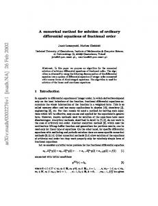
Chapter 1, p. 29]. It is easy to check that, because of (2.24), if Imz > 0, the straight half-line through the origin and z e S , joining z to oo, can be taken as the path /,. As for l2, we can take the circular arc with radius \z\ joining z to the point (\z\, 0) and then the real half line x > \z\ (see Figure 1). If Im z < 0, we interchange the roles of /( and l2. Therefore, we have
(2.26) (2.27)
F(z) = a~l/2 j* Q(t)dt, Vlz'00(F)oo in S , and the parameter a, as a —>+oo. This fact is related to the well-known double asymptotic nature of the Liouville-Green approximations [10, Chapter 6]. At this point, we construct the real Liouville-Green basis, i.e., a linear combination of U(z) and V(z) which is real on the real axis. Recalling that V(x) = U(x) (cf. [10, Chapter 6]), we obtain the real basis
(2.30)
u(x) = ReU(x),
v(x) = lmU{x).
License or copyright restrictions may apply to redistribution; see http://www.ams.org/journal-terms-of-use
NUMERICALMETHOD FOR EVALUATINGZEROS
Figure 1 "¿¡-progressive"paths in the z-planefor the case Imz > 0
It is clear now that u(x), v(x) can be holomorphically continued (in a unique way) into S
by the relations
_ U(z) + V(z) U(z)-V(z) v(z) 2 ' x /_= 2/ Correspondingly, the auxiliary function p), and in 5
, where u (z) + as well, provided
that (2.33)
u(z) + v2(z) = U(z)V(z) = a~l,2[l + ex(z)][l + e2(z)] ^ 0,
i.e., for |e (z)| < 1, j' = 1, 2 . This entails a possible restriction of S to an annular sector with a /arger value of p (but with unchanged angle). Below we
License or copyright restrictions may apply to redistribution; see http://www.ams.org/journal-terms-of-use
598
RENATO SPIGLER AND MARCO VIANELLO
shall use the same symbol for this modified sector. Equation (2.17) itself can be considered as a differential equation in S . We now obtain a preliminary asymptotic approximation for cf>(z)as z —► oo in S . Evaluating the (constant) Wronskian
(2.34)
W[u(z),v(z)]=\
through (2.20), we get from (2.32), (2.33), (2.29) (2.35)
cp(z) =-—£--—3 [l+ex(z)]2[l+e2(z)]2
= a[\ + 0(a~l/2zl-p)].
We can go further and improve this asymptotic approximation as follows. Using the asymptotic differentiation theorem [10, Chapter 1], we obtain from
(2.35) (2.36)
= q(t)+ [ht].
It is easily shown that cj>(t)= ß2(ßt) and n(t)= ß2n(ßt). Our objective is to approximate cj>,but we find it more convenient to first consider q\ and
then to go back to . Lemma 3.1. Let (3.7)
G(zx,z2,z,)
= q-\^
+ ^2
be a complex-valued function of the three complex variables zx, z2, z3, defined on the closed polydisc P = 7), x 7J>2 x D3, where Dx = B(c, e, ), 7J>2 = B(0, e2), and D3 = B(0, e3), with B(zQ, r) c C denoting the open ball with center in z0 and radius r and 0 < ex < c (c a positive constant), e2> 0, e3 > 0; ^eC is a constant. Then G is uniformly Lipschitz continuous in P,
(3.8)
\G(z)-G(n)\"n\}
=V3ßx-pa-l/2(ßa]/2)-2n
■0[(\t\-(n
+ l)V2)-l-p],
teSn+x.
In order to estimate || grad t7|| by Lemma 3.1, we have to estimate the radii of the component discs of the polydisc. We have
|0n(O- ß2a\< |0(O- ß2a\+ |0„(O- 0(01 < ß2-pO(fp)
+ ß[-pa-i/2(ßal/2r2nO((\t\
- nV2)~l-p),
111
and then, as ßa ' > 1, the estimate -p-V
>■ ..< ^ n2-p„¡ (3.24') |0n(O-/ra|n+xis holomorphic in Sn+X. We then claim x < (v/3/4)/(c - e3) (c = ß a), i.e., we can choose £, and e2 in such a way that the other two components of grad G are estimated by ^(l/ß2a). This can be done again, because fi is infinitesimal, for xQ sufficiently large, say x0 > x'0'. We conclude that
(3.29,
XS«fc
and hence, by Lemma 3.1, using (3.21) and (3.23), we get
(3.30)
(;V/2)
2"0[(|/| - (« + 1)n/2)
"]
3 £2a = ßl-pa-i/2(ß2a)-(n+l)0[(\t\
- (n + i)V2)-l~p],
t e Sn+X,
provided that x0 > max{//, x'0, x0'} . This value of x0 depends, in general, on all parameters entering the problem (except ß). Comparing (3.30) with (3.20) and going back to the variable z, it is clear that the inductive proof is complete. D Some observations are now in order. In the proof above, the condition 2 —1/2 ß a > 1 was needed. The transformation z - ßt with ß > a ' is therefore
License or copyright restrictions may apply to redistribution; see http://www.ams.org/journal-terms-of-use
RENATOSPIGLER AND MARCOVIANELLO
604
instrumental in reducing equation ( 1.1) to an equation to which the algorithm (3.1) can be applied when a < 1. Moreover, it is clear from (3.16) that the larger ß a the faster the "convergence" of the algorithm. However, larger values of ß reduce the Re(0-interval for a given x-interval (x = Re(z)) in which we want to evaluate zeros. Therefore, the zeros are not so well separated when
we choose ß large. Going back to the z-variable, the vertices of the sectors Sn increase linearly with ß (and with «) ; cf. (3.15). This entails that the zeros lying outside Sn cannot be approximated by using the estimate in (3.16) for 0. As a corollary of Theorem 3.2, we can relate the desired accuracy to the number of iterations needed to attain it. Corollary 3.3. The number of iterations, «(e), needed to attain the accuracy e in the iterative scheme (3.1) is asymptotically given by „,,, , ., |loge| +
(3.31)
n(e)~
* »' , log(jffa)
e^O
,
uniformly in z, z e Sn,e,.
Proof. From (3.16), the condition
|0„(z) - 0(z)| < e, with \z\ - nß\[2 > x0
for all z in 5^, i.e., a-l/2(ß2a)-"0(x~l~p) (C - loge)/k>g(/? a) for some constant C, and thus choosing
In the next section, we shall numerically compute zeros of solutipns to equation (1.1) starting from the approximation cpn of the function 0. If we approximate 0 within an accuracy e , i.e., use 0n(£,, we "lose" zeros in the sense that our procedure is asymptotic in nature, and only those zeros lying in £„,., can be approximated. In fact, we get from [5, Chapter XI, Corollary 5.3, p. 348] the asymptotic estimate
(3.32)
x as x —>+00 n for the number of zeros in the interval (p, x). Using (3.31) in
,.„, 3.33)
N(p,x)~—
, ßy/2
and this in (3.32) with x = x,,, (3.34)
ßV2
xn(e) = x0 + -—7/i(fi)~-—r«(e 1' sin y sin y
we obtain
N(p, xn{e))~ A\loge\
as e -> 0+ ,
where
(3.35)
A=
,
ßy/2ä 7zsiny'log(ß2a)
License or copyright restrictions may apply to redistribution; see http://www.ams.org/journal-terms-of-use
NUMERICAL METHOD FOR EVALUATINGZEROS
605
This shows the advantage of our approach compared to the mere asymptotic approximation (0 - 0O = q). In fact, in order to obtain the same degree of accuracy, the latter requires x > x(e) = (Ba~ ' ) ' +p'e~ ' +p), where B is the constant in the 0-symbol in (2.38). We emphasize, finally, that our approach is not only better because of logarithmic growth as opposed to power growth as e —>0+ , but also because we made coarse estimates in obtaining (3.31). Better results could have been obtained by taking into account the z-dependence in
(3.16). Remark 3.4. Theorem 3.2 also holds for the more general class of carriers
,-,,,
(3.36)
q(z) = a + - + Q(z),
a>0,beR,
z
Q(z) = 0(z-p),
p>l.
This form allows us to include carriers having full asymptotic or convergent power series expansions in z~ like Z^oa/z_J ■^e can wfite
(3.37)
q \b\/2a, which amounts to selecting the principal branch of / ' (z). This entails, possibly, an increase of the radius p in the annular sector, S . Moreover, it turns
out that v[i ^ = 0(z~x), where X = min{p - 1, 1}, and then ej = 0(z~x),
^ , and thus in the estimates of e, and 0, depend in general on b (in addition to a, p, y, p, K, as before).
4. Numerical
examples
If a(x) denotes a Liouville-Green phase, then the relation (2.7) and the definition (2.18) ensure that the equation
(4.1)
a(xk)-a(x)=
f " (Pl/2(t)dt = n, JX
xk being any fixed zero, has the unique solution x = xk_x (relation (4.1) actually refers to the Liouville-Green basis (v , u)). In practice we solve, instead, equation
(4.2)
fk 4,f(t)dt-n = 0. JX
License or copyright restrictions may apply to redistribution; see http://www.ams.org/journal-terms-of-use
RENATO SPIGLER AND MARCO VIANELLO
606
In fact, we start from an approximation xh of a certain "large" zero, xh , and compute successively the approximate values of the smaller zeros xk, k = « - 1, « -2, ... , which are denoted by xk . The initial value xh must be supplied independently of our method. Moreover, throughout all of the procedure, the approximation 0n of 0 is used, the corresponding error being given
by Theorem 3.2. Therefore, in evaluating zeros of solutions to (1.1), we can identify two main steps. We have first to obtain an approximation 4>n of 0 (which is accomplished by Theorem 3.2, see the algorithm (2.15)), and then to solve equation (4.2). As for the first step, note that nturns out to be a rational function of q, q , ... , q( "' (cf. (2.15)), and one can take advantage of computer algebra techniques to get such a function explicitly. In fact, in the examples below, we used MACSYMA. Moreover, whenever q is given in terms of elementary functions, 0n is of the same type; in particular, if q is a rational function, cpn is also rational. Following this procedure, the numerator and denominator degrees of the rational functions involved in general increase exponentially with « , thus yielding exponential computational complexity. The convergence of the algorithm is, however, very fast (cf. (3.16)), so that accurate results are obtained in very few iterations. On the other hand, if we merely use numerical differentiations in (2.15), the propagation of the local truncation error cannot be controlled after a few iterations. In the examples below, the carrier q is given in terms of elementary functions; we then proceed as follows, combining conveniently symbolic manipulations and numerical evaluations in order to face only polynomial computational complexity.
It is easily seen that the evaluation of