ETNA
Electronic Transactions on Numerical Analysis. Volume 3, pp. 160-176, December 1995. Copyright 1995, Kent State University. ISSN 1068-9613.
Kent State University
[email protected]
A PARALLEL GMRES VERSION FOR GENERAL SPARSE MATRICES ∗ JOCELYNE ERHEL
†
Abstract. This paper describes the implementation of a parallel variant of GMRES on Paragon. This variant builds an orthonormal Krylov basis in two steps: it first computes a Newton basis then orthogonalises it. The first step requires matrix-vector products with a general sparse unsymmetric matrix and the second step is a QR factorisation of a rectangular matrix with few long vectors. The algorithm has been implemented for a distributed memory parallel computer. The distributed sparse matrix-vector product avoids global communications thanks to the initial setup of the communication pattern. The QR factorisation is distributed by using Givens rotations which require only local communications. Results on an Intel Paragon show the efficiency and the scalability of our algorithm. Key words. GMRES, parallelism, sparse matrix, Newton basis. AMS subject classifications. 65F10, 65F25, 65F50.
1. Introduction. Many scientific applications make use of sparse linear algebra. Because they are quite time consuming, they require an efficient parallel implementation on powerful supercomputers. An important class of iterative methods are projection methods using a projection onto a Krylov subspace. The aim of this paper is to study the parallelization of such methods for general sparse matrices. We chose to design and implement a parallel version of the GMRES algorithm [21]. The main part of GMRES is the Arnoldi process which generates an orthonormal basis of the Krylov subspace. The target architecture here is a parallel machine with a distributed memory. We chose a Single Program Multiple Data (SPMD) programming style where each processor executes the same code on different data. Data are distributed according to a static mapping and communications are expressed by means of messages. The parallelization of GMRES has been studied by several authors. Some of them consider the basic GMRES iteration with the Arnoldi process, for example in [11, 22, 3, 7]. Variants of GMRES such as α − GM RES [26] have also been designed. Hybrid algorithms combining a GMRES basis with a Chebychev basis are also investigated in [15]. Another approach is to define a new basis of the Krylov subspace as, for example, in [16, 8, 9, 10, 5, 2]. Our implementation is based on the ideas develop in [2]. It first builds a Newton basis which is then orthogonalized. This approach requires the parallelization of two steps: the basis formation which relies on matrix-vector products and the basis QR factorization. As far as the matrix-vector product is concerned, one of two classes of matrices are usually considered: regular sparse matrices arising for example from the discretisation of PDE on a regular grid and general sparse matrices with an arbitrary pattern of nonzeros. This paper deals with the second class. The parallelization of the sparse matrix-vector product in this case has been studied for example in [3, 4, 19]. Our present work uses the library P-SPARSLIB described in [20]. In our implementation, the QR factorization is done either by a Gram-Schmidt process as in [10] or by a Householder/Givens factorization as in [24]. ∗ Received Oct 2, 1995. Accepted for publication November 22, 1995. Communicated by L. Reichel. † INRIA-IRISA , Campus de Beaulieu, 35042 Rennes, France.
[email protected]
160
ETNA Kent State University
[email protected]
Jocelyne Erhel
161
The paper is organized as follows. The second part describes the basic sequential GMRES version. The third part is devoted to the parallelization of the Arnoldi process with a Newton basis. This involves two main procedures, the sparse matrix-vector product and the QR factorization. Their parallelization is studied in the next two parts. Numerical experiments in the sixth part first show the impact on convergence of the Newton basis. In particular, we exhibit a matrix where the ill-conditioning of the Newton basis degrades drastically the convergence. We then give performance results on a Intel Paragon parallel computer. Concluding remarks follow at the end. 2. Sequential version. We first recall the basic GMRES algorithm [21]. Consider the linear system Ax = b with x, b ∈ Rn and with a nonsingular nonsymmetric matrix A ∈ Rn×n . The Krylov subspace K(m; A; r0 ) is defined by K(m; A; r0 ) = span(r0 , Ar0 , . . . , Am−1 r0 ). The GMRES algorithm uses the Arnoldi process to construct an orthonormal basis Vm = [v1 , . . . , vm ] for K(m; A; r0 ). The full GMRES method allows the Krylov subspace dimension to increase up to n and always terminates in at most n iterations. The restarted GMRES method restricts the Krylov subspace dimension to a fixed value m and restarts the Arnoldi process using the last iterate xm as an initial guess. It may stall. Below is the algorithm for the restarted GMRES. Algorithm 0: GMRES(m) ǫ is the tolerance for the residual norm ; convergence = false ; choose x0 ; until convergence do r0 = b − Ax0 ; β = kr0 k ; * Arnoldi process: construct a basis Vm of the Krylov subspace K v1 = r0 /β ; for j = 1, · · · , m do p = Avj ; for i = 1, · · · j do hij = viT p ; p = p − hij vi ; endfor ; hj+1,j = kpk2 ; vj+1 = p/hj+1,j ; endfor ; * Minimize kb − Axk for x ∈ x0 + K * Solve a least-square problem of size m compute ym solution of miny∈Rm kβe1 − Hm yk ; xm = x0 + Vm ym ; if kb − Axm k < ǫ convergence = true ; x0 = xm ; enddo The matrix Hm = (hij ) is a upper Hessenberg matrix of order (m + 1) × m, and we get the fundamental relation AVm
= Vm+1 Hm .
The GMRES algorithm computes x = x0 + Vm ym where ym solves the least-squares
ETNA Kent State University
[email protected]
162
A parallel GMRES version for general sparse matrices
problem miny∈Rm kβe1 − Hm yk. Usually a QR factorization of Hm using Givens rotations is used to solve this least-squares problem. The linear system can be preconditioned either at left or at right solving respectively M −1 Ax = M −1 b or AM −1 (M x) = b where M is the preconditioning matrix. The most time-consuming part in GMRES(m) is the Arnoldi process. Indeed, the solution of the small least-squares problem of size m represents a neglectible time. The Arnoldi process contains three operators: sparse matrix-vector product, orthogonalization and preconditioning. We now study the parallelization of the Arnoldi step. 3. Parallel Arnoldi process. The Arnoldi process builds an orthonormal basis of the Krylov subspace K(m; A; r0 ). It constructs the basis and orthogonalizes it at the same time; as soon as a new vector is added, it is orthogonalized relative to the previous vectors and normalized. The modified Gram-Schmidt algorithm is usually preferred for numerical stability. This leads to heavy data dependencies as shown in Figure 3.1. T i,j
(dot product and orthog.)
j
5
j
5
T 0,j (matrix-vector product)
T j+1,j (normalisation)
1 1
1
5
Arnoldi-MGS
i
1
5
i
Newton-Arnoldi
Fig. 3.1. Dependency graph of Arnoldi method
Some authors such as [22] have considered a classical Gram-Schmidt version to remove some dependencies, but in that case orthogonalization must then be done twice to ensure numerical stability. Another solution is to replace the Gram-Schmidt process by Householder transformations as in [25]. This provides a more accurate orthogonal basis at the price of more operations. Parallelism can be achieved using a Householder factorization by blocks [12]. In [16], the basis is built in blocks of size s, each new block being orthogonalized with respect to all previous s-vectors groups. But the convergence becomes slow with this approach. The solution which we have chosen, advocated for example in [14, 5, 1, 2], is to divide the process into two steps: first build a basis then orthogonalize it. Indeed, it removes the data dependencies on the left so that many tasks are now independent (Figure 3.1). The first step is merely a succession of matrix-vector products and the second step an orthonormalisation process.
ETNA Kent State University
[email protected]
163
Jocelyne Erhel
Nevertheless, the basis must be well conditioned to ensure numerical stability (more precisely, to avoid loss of orthogonality and to ensure a well conditioned leastsquares reduced problem). Following [2], we choose here a Newton basis defined by (3.1)
Vbm+1 = [σ0 v, σ1 (A − λ1 I)v, ..., σm
m Y (A − λl I)v]. l=1
The values λl are here estimations of eigenvalues of A ordered with the Leja ordering. We compute m Ritz values in a first cycle of GMRES(m) and order them in a Leja ordering, grouping together two complex conjugate eigenvalues. We then have a basis with normalized vectors of the Krylov subspace Vem+1 such e m+1 . We compute an orthonormal basis with a QR factorization that Vbm+1 = Vem+1 D (3.2)
˜ m+1 , ˜ m+1 R Vem+1 = Q
so that we can write (3.3)
b e m+1 R, AVbm = Q
b ∈ R(m+1)×m is an upper Hessenberg matrix which is easy to compute. We where R end up with a minimization problem similar to that of GMRES with the function J defined by (3.4)
b J(y) = kβe1 − Ryk.
To reiterate, we have a new version, called NewtonGMRES(m), which offers more parallelism and which is summarized below: Algorithm 0: NewtonGMRES(m) ǫ is the tolerance for the residual norm ; * Initialisation Apply algorithm 2 to find an approximation x0 and a Hessenberg matrix m × m, Hm ; Compute eigenvalues λ(Hm ) = {λj }m j=1 and order λj in a Leja ordering ; convergence = false ; * Iterative scheme until convergence do Compute Vem+1 ; em+1 ; e m+1 R Compute the factorization Vem+1 = Q b b b e Compute R such that AVm = Qm+1 R ; b and find ym solution of (3.4) ; Compute the QR factorization of R, e m ym ; Compute xm = x0 + Vem D if kb − Axm k < ǫ convergence = true ; x0 = xm ; enddo NewtonGMRES(m) contains two main steps: the computation of the basis Vem+1 which involves matrix-vector products and its QR factorization. We now analyze the parallelization of these two procedures.
ETNA Kent State University
[email protected]
164
A parallel GMRES version for general sparse matrices
4. Parallel sparse matrix-vector product. The computation of Vem+1 involves operations of the type y = σ(A − λI)x. Without loss of generality, we study here the matrix-vector product y = Ax. For sparse matrices, a natural idea is to distribute the matrix by rows and to distribute the vectors accordingly. Since the vector x is updated in parallel in a previous step, it induces communication to compute y. A straightforward implementation would broadcast the vector x to each processor so that each processor gets a complete copy. However, communication can be drastically reduced thanks to the sparse structure of the matrix A. To compute the component y(i) only a few components x(j) of x are required, namely those corresponding to nonzero entries aij in row i. Moreover some of these components are local to the processor. These two remarks are the basis for the distributed algorithm designed by Saad [19]. Let us denote by xloc and yloc the vector blocks distributed to the processor. Local rows are the rows allocated to the processor and local columns refer to local components of vectors. Other columns are called external and we denote by xext the set of external components required. We also denote by Aloc the matrix block with local row and column indices: (4.1)
Aloc = {aij : yi is local and xj is local},
and by Aext the matrix block with local rows but external columns: (4.2)
Aext = {aij : yi is local and xj is external}.
This block structure is depicted in figure 4.1.
External
A ext
Aloc
Local A ext
External
Fig. 4.1. Distributed matrix
The matrix-vector product is then written (4.3)
yloc = Aloc ∗ xloc + Aext ∗ xext .
ETNA Kent State University
[email protected]
Jocelyne Erhel
165
The processor must then receive xext from other processors before processing the second term. Converserly, it must send its components to other processors requiring them. The communication pattern is set up in an initialization phase on each processor and stored in data structures. This step requires, on each processor, the knowledge of the distribution of the rows and the local matrix. Each processor has a list jsend(p) of components which will be sent to processor p and a list jrecv(q) of components which will be received from processor q. More details can be found in [20, 17]. Since the matrix is processed by rows, a storage by rows is mandatory. We use a classical compressed sparse row (CSR) format. Each local matrix is stored using a local numbering with a correspondance between local and global numbers. Finally we get the following distributed algorithm, executed on each processor: Algorithm 0: Distributed sparse matrix-vector product Send xloc [jsend(p)] to processors p ; Compute yloc = Aloc xloc ; Receive x[jrecv(q)] from processors q and build xext ; Compute yloc = yloc + Aext xext ; This algorithm allows communication to overlap with computations and is scalable because the volume of communication increases much slower than the volume of computation with the size of the problem. The amount of communication depends on the size of each external block. Renumbering techniques help to reduce this size. They are based on graph partitioning heuristics applied to the adjacency graph of the matrix. The objective is to reduce the size of the interfaces and to balance the size of each subgraph. 5. Parallel QR factorization. The other procedure of the Newton-Arnoldi em+1 . e m+1 R method is the factorization Vem+1 = Q We have to design a parallel QR factorization of a matrix V which is rectangular of size (m+1)∗n with m