A Parallel Matrix Inversion Algorithm on Torus with Adaptive Pivoting Javed I Khan, Woei Lin, & David Y. Y. Yun East West Center & Department of Electrical Engineering University of Hawaii at Manoa 2540 Dole Street, Honolulu, HI-96822
[email protected] Tel:808-956-7249 Fax:808-941-1399
ABSTRACT
This paper presents a parallel algorithm for matrix inversion on a torus interconnected MIMD-MC2 multi-processor. This method is faster than the parallel implementations of other widely used methods namely Gauss-Jordan, Gauss-Seidal or LU decomposition based inversion. This new algorithm also introduces a novel technique, called adaptive pivoting, for solving the zero pivot problem at no cost. Our method eliminates the costly row interchange used by the existing elimination based parallel algorithms. This paper presents the design, analysis and simulation results (on a 32 Node Meiko Transputer) of this new and efficient matrix inversion algorithm. August 14, 2001 Published in the Proceedings of the 21st International Conference on Parallel Processing, ICPP’92 St. Charles, Illinois, August 1992, pp69-72
A PARALLEL MATRIX INVERSION ALGORITHM ON TORUS WITH ADAPTIVE PIVOTING Javed I. Khan, Woei Lin & David Y. Y. Yun East West Center & Department of Electrical Engineering University of Hawaii at Manoa, Honolulu, HI-96848
[email protected] This paper presents a parallel algorithm for matrix inversion on a torus interconnected MIMD-MC2 multiprocessor. This method is faster than the parallel implementations of other widely used methods namely Gauss-Jordan, Gauss-Seidal or LU decomposition based inversion. This new algorithm also introduces a novel technique, called adaptive pivoting, for solving the zero pivot problem at no cost. Our method eliminates the costly row interchange used by the existing elimination based parallel algorithms. This paper presents the design, analysis and simulation results (on a 32 Node Meiko Transputer) of this new and efficient matrix inversion algorithm.
1 Introduction Csanky [1] has shown the best possible bound of parallel matrix inversion. Given a finite number of processors, the best we can do is to compute inverse in O(log2n) time using O(n4/log n) processors. However, such processor requirement is unrealistic. Among the O(n) algorithms, using O(n2) processors, QR method using Givens transformations [4] takes more than 8n computational steps (because of decomposition), LU decomposition requires 3n steps (because of forward and backward substitutions), Gauss-Jordan requires 2n steps (because of backward substitution) and Gauss-Seidal requires n steps, but its step-width is 4flops (because it maintains two matrices) [4]. We here propose a new parallel algorithm, which is superior to all of the above methods, and is able to compute the inverse by performing n3 computations in n sequential steps on n2 processors with 2flops step-width. This algorithm is based on Faddeeva’s [2] method for the computing determinant. We have reduced the matrix inversion problem to the problem of computing determinants, and mapped the transformed computations on a torus architecture with overlapped computational phases. As we will see, the perfect match between the algorithm and the homogeneous torus structure resulted in a highly localized and uniform communication and computation pattern. Two of the most critical problems in matrix manipulation are zero pivots and propagation of rounding off error [5]. Some researchers suspect the existence of a law of conservation in linear systems which states that if a stability criterion is to be met then a certain number of arithmetic steps must be performed [4]. Existing matrix algorithms use row column interchange for stability. But, in parallel computation such interchange is prohibitively expensive due to communication cost. Our algorithm solves the problem of zero pivot by dynamic adaptation of pivots and re-labelling of elements using local informations. Thus, it substitutes the costly row column interchange at no cost. Sections 2 and 3 respectively present the theoretical derivation of the computational procedure and the supporting theorems for adaptive pivoting. Sections 5 and 6 respectively present the algorithm and the simulation study performed on a 32 node Meiko Transputer.
2 Inversion Method Computing Determinants: We shall start from the Faddeev’s original procedure [2]. Given the nxn matrix A, if a11 ≠ 0 then the determinant is, a11a12a13…a1n a22.1a23.1…a2n.1 a a a …a 21 22 23 2n a a …a 3n.1 32.1 33.1 | A| = ⋅⋅⋅⋅ = a11* = a11*A.1 ⋅ ⋅ ⋅ ⋅⋅⋅⋅ an2.1an3.1…ann.1 a a a …a nn n1 n2 n3
Here, the subscript .n refers to the successive stages after each Gaussian elimination. i.e., aij.1=aij.0-ai1.0 a1i.0/a11.0. i,j= 2,3,...n. One such elimination along the rows (or columns) of matrix A reduces the original determinant to a product of pivot a11 and a determinant of (n-1)th order matrix A.1. Repeated application of the above transformation generates matrices of decreasing orders and corresponding coefficients a11, a22.1 ...ann.n-1. Finally, the determinant of the matrix is given by the scalar equation (1) provided all the pivots are non-zero. | A| = a11*a22.1*a33.2*…ann.n − 1
(1)
Computing Inverse: The cofactor Aij of the element aij is the determinant of a new (n-1)x(n-1) matrix formed by the elements of A except the ith row and jth column. However, this same cofactor Aij can be defined as the determinant of another matrix E of order (n+1)x(n+1), which is constructed by augmenting (instead of eliminating) a new row and a new column with A in the following way, a11 a 21 ⋅ E = ⋅ a n1 e(n + 1)1
a12 a22 ⋅ ⋅ an2 e(n + 1)2
… …
… …
a1n a2n ⋅ ⋅ ann e(n + 1)n
e1(n + 1) e2(n + 1) e3(n + 1) e(n + 1) (n + 1)
where, e pq = a pq
when1 ≤ p ≤ n, 1 ≤ q ≤ n
= 1 when
p = (n + 1), q = i
= 1 when
p = j, q = (n + 1)
= 0 else
Now, n times repeated application of the Faddeeva’s procedure (just described above in Sec-2.1) on E generates a new matrix A.n =[aij.n] such that: −Aij = a11*a22.1*a33.2..*ann.n − 1*aij.n = | A| aij.n
(2)
Equation-(2) and Cramer’s rule directly shows that −A is the inverse of A as shown below: T .n
A−1 =
1 | A|
A11 A 21 ⋅ * ⋅ ⋅ An1
A12 A22 ⋅ ⋅ ⋅ An2
A13 A23 ⋅ ⋅ ⋅ An3
… …
…
A1n a11.n a A2n 21.n ⋅ ⋅ = − ⋅ ⋅ ⋅ ⋅ Ann an1.n
a12.n a22.n ⋅ ⋅ ⋅ an2.n
a13.n a23.n ⋅ ⋅ ⋅ an3.n
… a1n.n T … a2n.n ⋅ ⋅ ⋅ … ann.n
Computational Model & Mapping The following procedure computes Equation-(2):
1. Enter the first phase k=1. Take the original matrix [aij] and create the extended matrix E1 with eij =aij for i,j=1,2..n. 2. Add a new row and a new column with all zero elements except, e(n+1),1.k =-1 and e1,(n+1).k=1. 3. Calculate ei,j.1=ei,j.1-ei,1.1*e1,j.1/e1,1.1 for all i,j= 2,..(n+1). 4. Consider the elements eij.k of Ek with i and j varying from 2 to (n+1) as the elements ei,j.k+1 of the new extended matrix Ek+1. 5. Repeat steps 2,3 & 4 until k=n. At the end of nth phase, the inverted matrix is given by [eii.n]T. Fig-1 presents the propagation of computation plane by the above model for a 4x4 matrix. In each of the phases, the elimination is performed on the shaded elements. The lower right 4x4 elements at the end of 4th phase contain the transpose of the inverse.
PHASE PIVOT
Phase 1
Complete Taurus
Phase 3
Phase 2
Phase 4
Fig-3 logical mesh containing the active matrix is wrapped and iii). the phase procedure is required to slide down the diagonal at every iteration. We have used torus to accommodate all the phases as shown in Fig-3. Because of its boundary free property, it maps uniformly all the wrapped around meshes. The phase computation and communication pattern presented in Fig-2, applied recursively on the logical meshes of Fig-3 provides a compact mechanism for matrix inversion.
3 . Dynamic Adaptive Pivoting E
AS
PH PA
O
PR N
IO
AT
G
(a) PHASE 1
(b) PHASE 2
(c) PHASE 3
(d) PHASE 4
Fig-1 [P=V]
[U1=V]
[U2=V]
[U3=V]
v=1/V
v=V/P
v=V/P
v=V/P
P
P V
P U/V
U/V
U/V
[L1=V] v=-V/P
v=V-U1*L1/P v=V-U2*L1/P v=V-U3*L1/P
L
L V
L U/V
U/V
U/V
[L2=V] v=-V/P
v=V-U1*L2/P v=V-U2*L2/P v=V-U3*L2/P
L
L V
L U/V
U/V
U/V
[L3=V] v=-V/P
v=V-U1*L3/P v=V-U2*L3/P v=V-U3*L3/P
(a) COMPUTATIONS IN A LOGICAL PHASE
L
L
L
(b) COMMUNICATIONS IN A LOGICAL PHASE
Fig-2 Fig-2(a) shows the required computations in each of the phases. Capital letters denote the previous value and small letters denote the new value of the local variables. To perform these computations, each of the top row and left column nodes requires only one external data (the pivot), while all others need three external data i) the pivot, ii) the left most element of the row and iii) the topmost element of the column. We have reduced the number of communication from three to two by making the pivot transfer implicit. The topmost nodes, upon receiving P, transmit U/P instead of U and the nodes compute v=V-L*[U/V]. Fig-2(b) shows the resulting communication pattern. Now, we will map the phases. It is evident from the computational model (Fig-1) that the phase computation directly maps onto a mesh. However, between the phases, the corner of the computation frame slides down diagonally. A straightforward mapping on the mesh architecture therefore requires that all of the elements be pulled up diagonally one step in between phases. Algorithmically, this mapping is sound, but pulling the whole matrix up is expensive, and fortunately, can be avoided. At the end of each phase, the data of some nodes are no longer being used ( the first row and the first column) while, on the other hand, some new nodes are required (in the bottom). We have decided to map these new elements directly on the emptied nodes. The consequences are, i). the diagonal transfer of the entire matrix is no longer required, ii). the
In this section we show that it is possible to compute the inverse using more flexible pivot ordering than the principle-diagonal pivot order used earlier in section 2 (or in conventional algorithms). We know, a complete computation requires n pivots. In this section, using the following two theorems, we will show that any element can be a part of those n pivots so far no two are from the same row or same column. Thus, there can be n 2*(n 2 − 2n + 1)*(n 2 − 4n + 4)*(n 2 − 6n + 7)*….*2*1 ways of selecting the pivots. Below, a ⇐ b refers to a ’maps’ b.
Theorem 1: If T is a torus where individual processors are tij and B is A-T with elements aij and P is a set of n pivots, then the sequence of selecting individual pivots from the same set in successive phases does not affect the final mapping of the elements of B on the processors of the torus T where P is as follows and xi and yi are the pivot position selected in ith iteration: P = Px1y1, Px2y2, …Pxn yn ∋ x1 ≠ .. ≠ xn , 1 < xj < n, y1 ≠ .. ≠ yn , 1 < yj < n
Proof: To prove the above theorem we will show that the interchange of the lth and (l+1)th pivots, i.e. the sequences (i). …Pxl yl → Pxl + 1yl + 1 → .. and (ii). …Pxl + 1yl + 1 → Pxl yl → …, both generates the same result at the end of (l+1)th phase. Let, at the end of (l-1)th phase, the matrix be as follows where P and Q are the next two successive pivots and Tij is an arbitrary element of the torus. ⋅ ⋅ ⋅ A.l − 1 = ⋅ ⋅ ⋅ ⋅
⋅ ⋅
⋅ Pxl yl
⋅
⋅ ⋅
Uxl j
⋅
⋅
Nxl yl + 1
⋅
⋅ ⋅
⋅ Li y l
⋅
⋅ ⋅
Tij
⋅
⋅
Ri yl + 1
⋅
⋅
⋅ ⋅ Vxl + 1 j
⋅
⋅ Qxl + 1 yl + 1
⋅ ⋅ ⋅ Mx l + 1 y l ⋅
⋅
⋅
⋅
⋅ ⋅ ⋅
The sequence (i) …Pxl yl → Pxl + 1yl + 1 → ..computes the following at the end of (l+1) th phase on Torus node Tij.(l+1): UL VRP + LUQ − LVN − RUM NL V − P − R − Tij.l + 1 ⇐ T − =T− P P Q − MN PQ − MN UM
P
The other sequence (ii) …Pxl + 1yl + 1 → Pxl yl → …at the end of (l+1)th phase computes on the same node Tij.(l+1): LUQ + VRP − LVN − RUM RM U − Q VR − L − =T− Tij.l + 1 ⇐ T − MN Q Q P− PQ − MN VN
Q
These two values are same. Thus, if pivot set P is fixed, the sequence does not effect the final mapping.
Theorem 2: If B is A-T, and initially the matrix A is mapped onto torus T in such a way that aij is mapped on Tij for i,j=1,2,3....n and Plm and Pxy are two members of the pivot set P, then at the end of the nth phase, Tmx contains bly and Tyl contains bxm. Proof: Let us consider the general pivot order, P = {Px1y1, Px2y2, …Pxn yn ∋ x1 ≠ .. ≠ xn , 1 < x j < n, y1 ≠ .. ≠ yn , 1 < y j < n}
Since, the internal sequencing of the pivots does not effect the final mapping (according to Theorem 1), we will sort the pivots along row dimension. Let the resulting equivalent sequence be:
proceeds through the same diagonal, according to Theorem 1, the mapping expected from the forward diagonal pivot order will be preserved. Tracing: Flexible pivoting destroys the expected element-processor mapping. Since, all the processors know both the pivot selection strategies algorithmically, therefore, all can determine the physical position of the current pivot locally. Thus, according to theorem 2, a processor in the same row (or same column) as with a pivot, records the phase number as the final column (or row) position. This scheme provides the final mapping. Interestingly this mapping is done using only local information. Below we present a simplified pseudo-code of the algorithm. For clarity we have assumed the actual pivot order is supplied by the xphase[] and yphase[] arrays.
P˙ = {P1z1, P2z2, …Pnzn ∋ z1 ≠ z2 ≠ .. ≠ zn , 1 < z j < n} ≡ P
Since, at each of the successive phases a new column and a new row of the final matrix A.n are introduced. Thus, the kth column of the final matrix will contain the values of the cofactor of the rows calculated at the kth phase. Therefore, the ith column in A.n will contain the cofactor of the elements of the zith row. Now, to find out the content of a row, we again sort the pivots along the column dimension. Let the resulting equivalent sequence be the successive elements of the pivot set P¨ P¨ = {Pw11, Pw22, …Pwnn ∋ w1 ≠ w2 ≠ .. ≠ wn , 1 < w j < n} ≡ P
The above sequence maps the cofactor of the wjth column in the jth row. Thus, if plm and pxy are two pivots, then, i. lth column of T ⇐ mth row of A-1 ≡ mth column of B. ii. xth column of T ⇐ yth row of A-1 ≡ yth column of B. iii. mth row of T ⇐ lth row of A-1 ≡ lth column of B. iv. yth row of T ⇐ xth row of A-1 ≡ xth column of B. The following required mappings are the direct consequence of the above: Tml ⇐ blm ≡ Aml ; Tmx ⇐ bly ≡ A yl ; T yl ⇐ bxm ≡ Amx ; Txy ⇐ bxy ≡ A yx
4 . The Algorithm The algorithm proceeds through successive overlapped wavefronts. At each of the execution phases, the algorithm selects a pivot and then the computational wave, originating at the pivot, follows the computation and communication pattern explained in Fig-2. Pivots are selected according to a flexible default order. If a zero pivot is encountered, the default order is interrupted and a new pivot position is tried according to a search order. Default Order: According to Theorem 1 & 2 any n pivots can be selected in any sequence to compute the inverse elements as long as no two of them are from the same row or same column. The performance of the wave algorithm depends on the inter phase gap. Therefore, the pivot sequence for the default order should be chosen such that, this gap is minimum. Therefore, any of the diagonal orders is a good choice as a default pivot order. Search Order: The search for a non zero pivot can proceed along the i) same row, ii) same column or iii) same diagonal. Any three of the strategies can be adopted. If it proceeds through the same row (or column) than the singularity can be detected efficiently. On the other hand, if it
int k=0, s=n, p_count=n; int xphase[],yphase[]; getpid(i,j);
else v=v/p; send(v:east); send(p:south); }
/* Loop for n phases*/ while(p_count) { px= xphase[k]; py= yphase[k++];
/* If Left Column Elements*/ elseif(px==i) { send(v:south); recvb(p:west); if(p==ABORT) { xphase[s]=px; yphase[s++]=yx; p_count++; } send(p:east); v=-v/p;}
/* If Phase pivot*/ if(px=i and py=j) { if(v