A parameterization for flow separation in a river dune development ...

River, Coastal and Estuarine Morphodynamics: RCEM 2005 – Parker & García (eds) © 2006 Taylor & Francis Group, London, ISBN 0 415 39270 5

A parameterization for flow separation in a river dune development model A.J. Paarlberg, C.M. Dohmen-Janssen & S.J.M.H. Hulscher University of Twente, Water Engineering & Management, Enschede, The Netherlands

A.P.P. Termes HKV Consultants, Lelystad, The Netherlands

ABSTRACT: To simulate dune development, a model based on the two-dimensional vertical shallow water equations is applied to flume conditions. Realistic bedform behaviour of dunes with gentle slopes is obtained: dunes grow in amplitude, develop into asymmetric features and migrate. Due to a constant eddy viscosity in the model, flow separation cannot be treated explicitly. Therefore, a parameterization for flow separation is proposed, based on flume data. A parameterization is derived for the separating streamline, which is the upper boundary of the flow separation zone, and which can be used as bed level for flow computations. The shape of the flow separation zone is found to be independent of flow conditions, and is related to the height and local bed angle at the separation point, and to the angle of the separating streamline at the reattachment point. The parameterization is in reasonable agreement with flume data.

1

INTRODUCTION

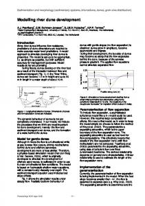
Accurate predictions of water levels during floods in rivers are essential in order to design an appropriate flood defence system or to determine effects of changes to the river system. Water levels during floods are largely influenced by bed roughness in the main channel of the river, resulting from flow over bedforms on the river bed (e.g. dunes, see Fig. 1). Such dunes develop during floods as a result of the increasing discharge, leading to a roughness with a dynamic character. The roughness due to river dunes is dynamic since (1) the roughness increases and decreases during a flood and (2) the roughness lags the discharge with maximum dune dimensions occurring later than the maximum discharge (e.g. Ten Brinke et al. 1999; Julien et al. 2002). River dunes cause an increase in hydraulic roughness compared to a situation with flat bed, because they protrude into the flow producing shear stress and turbulence. Due to the interaction between unidirectional flow in rivers, and the sediment transport, sinusoidal bedforms develop into asymmetric dunes with gentle stoss-sides and steep lee-sides, as explained by Exner (see Leliavsky 1955, p. 24–26). The lee-side of a dune may become so steep that the flow cannot follow the bed surface any longer, forming a flow separation zone (Fig. 1). When flow is turbulent and viscous (which is generally the case in rivers, and in the used flume experiments), the flow separates behind steep dunes

due to an increasing pressure gradient behind the dune (Chang 1970, Buckles et al. 1984). Avalanching at the lee-side results in a dune with a brinkpoint and a slope at the angle of repose which is about 30◦ for sand in rivers. The turbulence (eddies) generated in the socalled flow separation zone slows the flow down. This process is often referred to as form drag and can be regarded as an additional roughness due to dunes. The amount of turbulence (and thus roughness) caused by flow over dunes is strongly related to general flow conditions and the shape and size of the flow separation zone (see e.g. Vanoni and Hwang 1967). At present, there is still limited knowledge about river dunes and the resulting roughness, let alone about their development during floods. Several researchers proposed methods to predict dune dimensions (e.g. dune length and dune height), based on a range of parameters like flow strength, water depth or sediment size. Part of the proposed methods are empirically based (e.g. Julien and Klaassen 1995; Van Rijn 1984), while others are more theoretically based (e.g. Kennedy 1969; Onda and Hosoda 2004). All these methods are designed to calculate equilibrium dune dimensions in steady, uniform flow. In that case a unique dune height and dune length exist for each specific combination of flow characteristics and sediment properties. Other researchers tried to include the observed time-lag due to unsteady flow conditions, in their models to predict dune dimensions (e.g. Allen 1976 and

883

Figure 1. Schematic representation of a dune in streamwise direction, along with some general characteristics.

Fredsøe 1979). However, as shown by Wilbers (2004), none of these predictors is able to predict dune dimensions during several floods in the River Rhine in the Netherlands. Wilbers (2004) developed a calculation method to predict dune development under unsteady flow conditions, based on a method proposed by Allen (1976), in which it is assumed that dunes adapt to equilibrium dune dimensions (as if steady flow conditions were present) with an exponential relationship. Dune steepness and bed shear stress are important parameters in the calculation method and both primary and superimposed secondary dunes can be predicted. Although the calculation method is applied with success to three sections of the Rhine branches, a major drawback is that the method is not generally applicable. For every situation, initial dune dimensions have to be known and data are required to calibrate the adaptation constant. Furthermore, the method gives only limited insight in the physics behind dune development during floods. In this paper we describe an approach to simulate dune development, which is set up to be appropriate. With this we mean the following. In hydraulic models, the influence of roughness due to dunes is mostly not included. We aim to develop an appropriate prediction method for roughness caused by dunes, which (1) can be included in hydraulic models, (2) and contains no unnecessary details in the modelling. To start with, we only analyze average dune dimensions in our model, despite the fact that dune development has a strong stochastic behaviour (see e.g. Van der Mark et al. 2005). Further, detailed processes such as vertical sorting (see e.g. Blom and Parker 2004) are not yet included in the model. Our approach is based on the morphodynamic model of Németh (2003), which was developed to predict the evolution of offshore sandwaves. The sandwave behaviour that is predicted by the model, shows large similarities with the development of river dunes: when a unidirectional current is applied, the sandwaves migrate, grow, and become asymmetric. In this paper we test the applicability of this model to predict dune development under flume conditions. Since offshore sandwaves have relatively large dimensions (height of about 10 m and length of about 500 m) flow separation is not likely to occur in offshore conditions. Therefore, this process is not included in the model. However, for river dune

development the process of flow separation is very important. Various methods exist to enable detailed modelling of turbulence in the flow separation zone using direct numerical simulation. For example, Yoon and Patel (1996) adopted a k − ω turbulence model enabling a detailed computation of the flow in the separation eddy. Results were shown to be in general agreement with the experimental data ofVan Mierlo and De Ruiter (1988). Stansby and Zhou (1998) showed that the computation of the flow in the separation zone improved when a non-hydrostatic pressure (instead of hydrostatic) was applied. A disadvantage of such methods is that they are complicated and require much computational effort. To keep the model appropriate, we describe an approach to include flow separation in a parameterized way. In Section 2 the general model equations are discussed, followed in Section 3 by an analysis of the model, including a dimensional- and a stability analysis. Section 4 discusses the application of the model to dunes with a gentle slope, for which no flow separation occurs. The parameterization of flow separation is described in Section 5. Finally, the conclusions are presented in Section 6.

2

MODEL

The model that is used in this study is described in detail in Németh et al. (2002), Németh (2003) and Van den Berg and Van Damme (2005). The model is based on the model developed by Hulscher (1996). In this section the most important equations are mentioned. For the simulations described in the paper, both the numerical implementations of Németh (2003) and Van den Berg and Van Damme (2005) are used. For future research we focus on the latter implementation since this approach is more efficient regarding computational effort and has a more appropriate numerical discretization than the former implementation.

2.1 Flow model The model is based on the two-dimensional vertical (2DV) shallow water equations. The momentum

884

equation in x-direction (divided by water density ρ) and the continuity equation read:

at the bed and the bed shear stress, which is important for sediment transport, are represented correctly. Soulsby (1990) computed velocity profiles using various viscosity profiles over depth and bottom boundary conditions ranging from full slip to no slip. Results show that the velocity profiles vary only little for different settings. We believe this approach is appropriate for our goals.

The velocities in the x- and z- directions are u and w, respectively. The z-coordinate is directed upwards from the average bed, which is located at z = 0. The mean water depth is denoted by H , and the fluctuation in the average water level is denoted by ζ. This results in a total water depth of H + h + ζ, where h is the bottom disturbance on the average flat bottom. Further, t is time, and g and Av denote the acceleration due to gravity and the vertical eddy viscosity, respectively. For more details about the model, the reader is referred to Van den Berg and Van Damme (2005).

2.4

2.2

Boundary conditions

The boundary conditions at the water surface (z = H + ζ) are that there is no flow through the surface, and no shear stress at the surface:

The boundary condition at the bed surface is that there is no flow through the boundary:

2.3 Viscosity model and partial slip condition An eddy viscosity which is constant over the depth is applied. Since a certain velocity profile is present, this implies that at the bed both the horizontal and vertical velocity are not equal to zero. To allow for a velocity at the bed, but to still impose a friction, a partial slip condition is introduced using the partial slip parameter S. The following boundary condition couples the resistance at the bed with the flow velocity at the bed (ub ):

Sediment transport model and bed behaviour

Only bedload sediment transport is considered in the model, since this is assumed to be the main transport mechanism behind dune development. A general bed load formula according to Komarova and Hulscher (2000) is applied:

where Sb is the volumetric bed load transport. The proportionality constant α [s2 m−1 ] and the nonlinearity parameter b describe how efficiently the sand particles are transported by the bed shear stress (Komarova and Huslcher 2000). The parameter b is analytically determined as 0.5 [−], and α and the slope parameters λ1 [m2 s−2 ] and λ2 [−] are expressed by:

where  is the critical Shields parameter modelled by a constant of 0.047, s is the relative density of sediment equal to 2.65 and γ is equal to 1 for unidirectional river flow. The grain diameter is denoted by d [mm] and φs is the friction angle (the angle of repose) with tan (φs ) = 0.6 (i.e. φs ≈ 30◦ ). The scale factors for the bed slope mechanism λ1 and λ2 take directly into account that sand is transported more easily downslope than up-slope. The second bed slope factor has a more diffusive character. Bed evolution follows from sediment continuity:

3 ANALYSIS OF THE MODEL 3.1 Model set-up: parameter settings where τb is the bed shear stress. The slip parameter determines the resistance at the bed. When this parameter increases, the bed shear stress increases too. Using this approach, vertical velocity gradients

The slip parameter, as well as the eddy viscosity, are parameters which are difficult to estimate. Relationships for offshore conditions are derived by Besio et al. (2003) which depend on hydraulic conditions and the

885

0.1

0.1

0.08 Distance from bottom (m)

Distance from bottom (m)

0.08 Linear fit R2 = 0.97 0.06

0.04

0.02

0

Measurements Log. regression DA velocity Modelled profile

0.06

0.04

0.02

0

0.2

0.4

0 0.2

0.6

Shear stress (N/m2)

0.3

0.4

Horizontal velocity (m/s)

Figure 2. Shear stress distribution over depth in flume experiment T3 of Van Mierlo and De Ruiter (1988).

Figure 3. Measured and modelled velocity profile.

roughness of the seabed. For flume or river conditions such relationships do not exist. In the model, the slip parameter S and the vertical eddy viscosity Av from Eq. (6) have a direct relation with the velocity profile. Therefore, measurements of velocity profiles over a rough flat bed in flume experiment T3 of Van Mierlo and De Ruiter (1988) are used to calibrate these parameters. In the experiment, the water depth is 10 cm and the depth-averaged flow velocity is 0.38 m/s (Fr ≈ 0.38). Because of the used partial slip condition at the bottom boundary, no logarithmic velocity profile can be obtained. Therefore, we calibrate on the general shape of the velocity profile and on the value of the bed shear stress (which is important for sediment transport). Measured values of the turbulent u- and wvelocities can be used to obtain the measured shear stress distribution over the water column using:

(Equation (7)). The proportionality constant α is estimated using Equation (8) at 0.3. The sediment transport formula is developed to use in offshore conditions, and the exact behaviour of the slope parameters λ1 and λ2 under river or flume conditions is not known. Therefore, we choose to include only the slope factor with the most simple form (so λ1 , without bed shear stress dependency) and analyze the results using this approximation. For the grain size a typical value of 3 mm is used, resulting in λ1 ≈ 6 × 10−3 . It should be noted that this parameter will be changed in Section 3.3, after considerations based on a dimensional- and a stability analysis of the model equations.

where the overbar denotes time-averaging (over the turbulent timescale). The shear stress distribution shown in Figure 2 is found. For stationary flow, the shear stress distribution over the depth is linear (see e.g. Jansen et al. 1994). Linear extrapolation to the bed, results in a bed shear stress of 0.51 N/m2 . Calibration against the velocity profile and the bed shear stress results in S = 1.9 × 10−3 m/s and Av = 1.9 × 10−4 m2 /s. Figure 3 shows the comparison of the modelled and the measured velocity profile. The parameters that remain to be estimated are the empirical constants in the sediment transport formula

3.2 Dimensional analysis In this model, flow and sediment transport are decoupled because, in general, changes in the flowfield have a shorter timescale than morphological changes. This aspect is checked by performing a dimensional scaling analysis on the model equations. Table 1 shows the used scaling parameters. The length scale δ follows from scaling the momentum equation (1) using the characteristic scaling parameters from the table. Using the characteristic values for the parameters U , H and Av discussed in Section 3.1, this (horizontal) length scale is about 21 meter. A hydrodynamical timescale (TH ) can be derived from introducing the scaling parameters in Equation (3):

886

Table 1.

Scaling of variables.

Parameter x- coordinate z- coordinate Hor. velocity Vert. velocity Water surface Bed shear stress Bed level

Symbol x z u w ζ τ zb

0.1 Scale UH 2

δ = Av H U U Hδ = U 2 /g Av U H

H

Av H

Dimensions

0.08

m m m/s m/s m m2 /s m

0.06 0.04 0.02 0 1

2

3

4

⫺0.02

Similarly, a morphodynamical timescale (TM ) can be deduced from Equation (10) as:

Figure 4. Residual time-independent flow field over two identical dunes (sketched at bottom, not to scale). On the vertical axis is the waterdepth [m], and on the horizontal axis is the distance along the dune [m]. Unidirectional flow is from left to right. Image courtesy: Ruud van Damme.

resulting in the following ratio:

over a small sine-shaped bed disturbance. The basis instability mechanism is present: sediment is transport uphill. Since unidirectional flow is imposed, we observe an asymmetric of the cells in flow direction. For the numerical stability analysis, the numerical implementation of the model equation of Németh (2003) is used. This numerical calculation method solves the model using Chebyshev polynomials for one solitary dune. Figure 5 shows the results for different values of the parameter λ1 . Also results of the analytical stability analysis are included. Numerical and analytical computations agree well. A (constant) migration rate of about 10 m/day is found, and the growth rate ranges between zero and about 10 m/day. The migration rate is in general agreement (order of magnitude) with measurements in the Rhine (Wilbers 2004) and with flume measurements with floodwaves (Wijbenga and Van Nes 1986). The growth rate seems a little high compared to the same measurement data. In Figure 5, it can be observed that the behaviour is different for different values of the slope parameter λ1 . In Section 3.1, a value of 6 × 10−3 for this slope parameter was derived. When this value is used in the stability analysis, no growth is found, and every initial disturbance is flattened out over time. The formula used to derive the value of λ1 is derived from an analysis for the modelling of offshore sandwaves, while in river situations some important scaling factor are essentially different. From a dimensional analysis of the sediment transport equation used in the model, it follows that λ1 scales with a factor Av /(UH ) ≈ 1/200. Furthermore, in the floodwave flume experiments of Van Mierlo and De Ruiter (1988) the order of magnitude of the observed dune length was about 1 meter. According to Figure 5 this seems to fit with a value of λ1 = 6 × 10−5 . Therefore, in the following simulations this value is used.

For the parameters previously discussed, it follows that TM /TH ≈ 25, and for typical river conditions (using same values, but now H ≈ 10 m) this gives TM /TH ≈ 2.8 × 104 . This makes it acceptable to use a quasi-stationary approach as in the model. It should be noted that the vertical eddy viscosity also changes for a larger water depth (i.e. it probably becomes larger towards the water surface). 3.3

Stability analysis

A linear stability analysis gives the growth rate and migration velocity of small initial bed disturbances. The initially fastest growing wave length of bed perturbations is often also a good indication for the bed behaviour on the longer term (see e.g. Van den Berg and Van Damme 2005). Thus the stability analysis can give indications whether the model equations can be applied to flume conditions, and whether realistic migration rates and growth rates are found. Furthermore, the response of the equation to different parameter settings can be investigated. The linear stability analysis is performed both analytically and numerically, to verify the numerical model results. For the analytical approach, use is made of the method of Van Damme and Van den Berg (2005). A small sine-shaped disturbance of H with