where ut â Rm is the motor command control signal provided at time t. .... u1 negative, and suppose the random perturbations to be small enough that the.
A parameterless biologically inspired control algorithm robust to nonlinearities, dead-times and low-pass filtering effects Fabio DallaLibera1,4 , Shuhei Ikemoto2 , Takashi Minato4 , Hiroshi Ishiguro3,4, Emanuele Menegatti1 , and Enrico Pagello1 1
Dep. of Information Engineering (DEI), Faculty of Engineering, Padua University, I-35131, Padua, Italy 2 Dep. of Multimedia Engineering, Graduate School of Information Science and Technology, Osaka University, 565-0871, Suita, Osaka, Japan 3 Dep. of Systems Innovation, Graduate School of Engineering Science, Osaka University, 560-8531, Toyonaka, Osaka, Japan 4 ERATO, Japan Science and Technology Agency, Osaka University 565-0871, Suita, Osaka, Japan
Abstract. A biologically inspired control algorithm for robot control was introduced in a previous work. The algorithm is robust to noisy sensor information and hardware failures. In this paper a new version of the algorithm is presented. The new version is able to cope with highly non-linear systems and presents an improved robustness to low-pass filter effects and dead-times. Automatic tuning of the parameters is also introduced, providing a completely parameterless algorithm.
1
Introduction
Biologically inspired algorithms have been intensively studied in the robotics field. In particular, we focused on robotic control problems and in [4] we presented a simple biologically inspired control that is robust to environmental changes and noise. The algorithm takes inspiration from bacteria chemotaxis, the process by which bacteria [1, 10, 8] sense chemical gradients and move with directional preference toward food sources. Among the most thoroughly studied organisms with regards to chemotaxis we can certainly cite Escherichia Coli (E. Coli). This bacterium has only two ways of moving, rotating clockwise or counterclockwise [1]. When it rotates counter-clockwise the rotation aligns its flagella into a single rotating bundle and it swims in a straight line. Conversely clockwise rotations break the flagella bundle apart and the bacterium tumbles in place.
2
The bacterium keeps alternating clockwise and counterclockwise rotations. In absence of chemical gradients, the length of the straight line paths, i.e. the counter-clockwise rotations, is independent of the direction. Thus, the movement consists in a random walk. In case of a positive gradient of attractants, like food, E. Coli instead reduces the tumbling frequency. In other terms, when the concentration of nutrients increases the bacterium proceeds in the same direction for a longer time. This strategy allows biasing the overall movement toward increasing concentrations of the attractant. Such a simple mechanism works despite the difficulties in precisely sensing the gradient. Actually, the spatial gradients in concentration cannot be sensed directly due to the small dimensions of the bacteria, so temporal difference in the concentration is used to estimate the nutrient distribution. A wide spectrum of models, from a very abstract point of view to the modeling of the protein interactions are available in literature [9, 2, 7]. The movement of E. Coli was mimicked in robotics as well. In [5] it was shown that while gradient descent is faster for tracking a single source, biased random walks perform better in the presence of multiple and dissipative sources and noisy sensors and actuators. Furthermore the stochastic nature of the algorithm prevents it from getting stuck in local minima. However, the robustness to hardware damages and noisy sensory information achievable by biased random walk were not fully exploited. Expressly, in [5] the hardware already provides two basic movements, proceed straight and change direction randomly, and the biased random walk is performed at the behavior level. This approach limits the robustness for unexpected hardware failures. In fact, if due to a hardware failure, the behavior corresponding to such commands will be different from the expected one, the task will not be accomplished. Imagine for instance to have a mobile robot with two wheels powered by independent motors and that due to an encoder problem one of the motors starts to rotate in the opposite direction. In this case when the “go forward” motor command is provided the robot spins around itself and the target will never be reached. With our approach [4], instead, a biased random walk is executed directly in the motor command space, i.e. the behaviors themselves are determined online through the random walk. This gives great robustness in case of hardware failures since new behaviors that exploit the current hardware behavior are found online by biased random walk. For instance, in case of the encoder failure described, the robot would explore new motor commands, until it finds that rotating the motors in opposite directions the distance from the target can be decreased. Concretely in [4] the control of the robot reduces to the single equation ut+1 = ut + αsgn (∆At )
ut + βηt kut k
(1)
where ut ∈ Rm is the motor command control signal provided at time t. The equation is composed of two terms, a bias term bt = sgn (∆At ) kuutt k and a purposely added random perturbation ηt ∈ Rm , multiplied respectively by two scalar coefficients α and β.
3
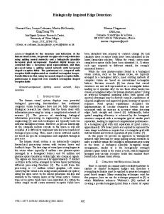
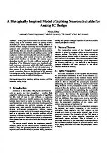
The quantity ∆At ∈ R appearing in the bias term expresses the variation of the “quality” of the robot state during the t-th time step. For instance, in [4] the task consists in reaching a red target, and the quantity ∆At represents the variation in the number of red pixels acquired by the camera image. Therefore, essentially, the bias term states that if the robot got closer to the target using command ut then command ut+1 should be similar. The second term is the most interesting part. In [4] it was shown that by adding random perturbations of opportune magnitude to the control input, it is possible improve the performances. Figure 1 reports an example. Let us suppose to have a holonomic robot initially placed at [10, 10]T (arbitrary units) that has to reach a target placed at [0, 0]T , and the motor command to be simply the translations along the two axes. If the perturbation is too small, then the effect of the bias will be strong, and even nearly tangential movements that bring the robot slightly closer to the goal will be used for a long time. If the perturbation is too big then the robot changes direction too frequently, even when the movement is headed straight to the goal. If the perturbation amplitude is appropriate than the robot will reach the goal with a good trajectory 5 . This result is confirmed observing the distribution of the robot heading direction compared to the optimal direction in Fig. 2. When the perturbation is too little essentially all headings that do not face backwards are chosen with uniform distribution. When the noise is too big, the robot tries all directions, with a small bias on the good ones. Finally, when the perturbation level is appropriate the distribution has a peak in the optimal heading. In [4] the robustness of the algorithm was highlighted by experiments both with a simulated and a real robot. In particular it was shown that the algorithm is able to drive to the target a simulated robot that undergoes substantial damages. Secondly real world experiments proved that even very noisy information can be used to accomplish the task. Results showed that the performance depends essentially just on the ratio between the two coefficient α and β, and not on their values itself. However, the optimal ratio depends on the hardware and environment conditions. The next section will highlight three shortcomings of the previous algorithm, and section 3 will present a new algorithm that faces these aspects. Furthermore a criterion to automatically adjust the perturbation level is introduced. Successively section 4 provides a quantitative comparison of the two versions of the algorithms, and finally section 5 concludes summarizing the paper and presenting future works.
2
Generality limitations of the previous version
In most systems opposite motor commands generate an opposite effects, at least in some regions of the motor command space, and that a scaled version of the motor command provides a similar effect with different intensity. Observing carefully Eq.1 it is possible to observe that the algorithm previous presented partially 5
A stochastic resonance effect can be observed. For details see [3, 6, 12].
4 6.36
6.34
distance traveled toward the target
6.32
6.3
6.28
6.26
6.24
6.22
6.2
6.18 −7
−6
−5
−4
−3 −2 −1 noise level [ln(β/α)]
β/α=0.07
0
1
β/α=6.60
12
start
10
12
start
10
8
8
6
6
6
4
4
Low perturbation magnitude
target
−2 −2
0
2
4
6
8
10
4
Approptiate perturbation magnitude
2
target
0
12
−2 −2
start
10
8
0
3
β/α=0.66
12
2
2
0
2
4
6
8
10
High perturbation magnitude
2
target
0
12
−2 −2
0
2
4
6
8
10
12
Fig. 1. Performance for different perturbation magnitudes. The top panel reports the performances for different values of β when α = 10−2 . The performance is measured as the average distance traveled toward the goal in 1000 time steps, calculated over 10000 simulations. The bottom panels report examples of trajectories obtained for different values of β. Precisely, the first trajectory was obtained for a low perturbation level, β = 0.07, the second trajectory corresponds to an opportune level of perturbation, β = 0.66 and finally the bottom right panel reports a trajectory generated with β = 6.6.
exploits this fact. In fact it assumes that if command ut is beneficial for the robot state at time t, then kuutt k will probably be a good bias for the following command ut+1 . Furthermore, if ut worsened the conditions during time t then it is assumed that − kuutt k will be an appropriate bias for ut+1 . These considerations however do not hold for many motor command spaces. Using the previous example, suppose again to have a holonomic robot whose coordinates are xt ∈ R2 . Assume now ut ∈ mathbbR2 and its two components � � to represent the velocity in 1 cos(u2t ) polar coordinates, i.e. xt+1 = xt + ut · . The non-linearity near the sin(u2t ) origin introduced by the cosine prevents the algorithm from being able to drive the robot to the goal. Another disadvantage of using −ut as bias when the conditions worsen is that the control algorithm performs badly if there are dead times in the response. Imagine for simplicity a unidimensional case where the goal is at +10 and the position xt , initially 0, changes by xt = xt−1 + ut−2 , xt , ut ∈ R. In this case the performance increases when the bias is positive. Suppose to start with u0 and u1 negative, and suppose the random perturbations to be small enough that the sign of the motor command ut is determined by the sign of the bias bt . Since
5 0.08 β/α=0 β/α=0.66 β/α=20.00
0.07
Probability Density Function
0.06
0.05
0.04
0.03
0.02
0.01
0 −180
−150
−120
−90
−60 −30 0 30 60 deviation from optimal heading [deg]
90
120
150
180
Fig. 2. Distribution of the robot heading, compared to the optimal heading, for different perturbation levels. The blue continuous graph reports the distribution for a low perturbation magnitude, the green dashed graph represents the probability density function obtained for an opportune perturbation coefficient (β = 0.66) and the third, red dotted curve, shows the distribution of the heading for an high perturbation level (β = 20).
u0 is negative ∆A2 will be negative, and the bias b2 and signal u2 will become positive. However, in the next step the effect of u1 will lead to a negative ∆A3 , which in turn will bring the bias b3 and u3 to become negative again. The effect of u2 will provide a positive ∆A4 , so the bias b4 will have the same sign of u3 , i.e. it will be negative. At this point the evolution of the bias will repeat, in a loop that contains two negative biases and a positive one. If the magnitude of the biases is similar for the positive and negative case, in general the bias will tend to bring the robot farther from the target instead of bringing it closer, and the system will never reach the target +10. Table 1 reports other examples of bias sequences that reveal to be a nuisance instead of being beneficial to reach the target. Table 1. Bias sequences leading to performance decrease u0 u1
Sequence ∆At -, -, +, . . . - ut +, -, -, . . . ∆At -, +, -, . . . - + ut -, -, +, . . . ∆At +, -, -, . . . + ut -, +, -, . . .
For similar reasons the bias can become deleterious if the system includes delays introduced by low pass filters. This can be a serious disadvantage of the
6
algorithm, since many physical systems present this kind of behavior. A simple example can be provided by introducing an Infinite Impulse Response filter in the example of a holonomic robot moving on the plane. Concretely, assume the robot to change its position by xt+1 = xt + vt where vt = (1 − 10−ρ ) · vt−1 + 10−ρ · ut . Let us define a “bad bias” a bias that has a heading that differs more than 90 degrees from the optimal one and would therefore bring the robot further from the goal. Figure 3 reports how the probability of bad biases changes by varying the random perturbation level (β/α ratio) and the delay level (ρ). Although the probability of bad biases can be minimized by changing the random perturbation level, it can be observed that as the delay increases the probability increases. For instance, for a value of ρ equal to 3 the probability of bad biases cannot be lower than 0.09.
2 0.45
1.5
0.4
noise level (log10 (β / α))
1
0.35
0.5
0.3
0
0.25
−0.5
0.2
−1
0.15
−1.5
0.1
−2
0.05
−2.5 0
0.5
1
1.5 delay (ρ)
2
2.5
3
Fig. 3. Probability of biases that would bring the robot further from the goal. The X axis represents the delay level (ρ), the Y axis represents the perturbation level (β/α) and the color indicates the probability of bad biases (lighter color indicates a higher probability). The yellow line indicates the noise level that gives the lowest bad bias for each delay level.
It is worth noting that for a wide range of problems it is often possible to find expedients that allow to mitigate the weak points presented in this section and that allow to use the previous version of the algorithm. In fact, adopting an adequate motor command space reveals to be sufficient in most of the cases. However, this paper aims at showing that the generality of the algorithm can be greatly improved without increasing the algorithm complexity.
3
A new version of the algorithm
As reported in the introduction, Escherichia Coli proceeds by movements in random directions, but when moving toward increasing concentrations of nutrients the movement in that direction is prolonged. A similar behavior can be obtained by taking ut+1 = ut if ∆At ≥ 0 and selecting ut+1 randomly6 if ∆At < 0. As in 6
In the following we assume to select ut ∈ Rm using a uniform distribution over the whole motor command space, but the results remain essentially the same using different distributions.
7
the previous version of the algorithm, a random perturbation can improve the performances. In particular, it is sufficient to add a perturbation to each of the components of the input when ∆At ≥ 0, i.e. uit+1 = uit + η i R, R ∼ N (0, 1) for each of the components of the input (1 ≤ i ≤ m). Choosing the bias at random when the system is getting further from the goal removes any assumption of linearity of the system. Clearly this leads to a performance decrease for systems that are effectively linear, but considerably improves the generality of the algorithm. Furthermore, in case of dead times periodic bias sequences with negative effects are unlikely generated. For instance, in the case of the unidimensional example provided in the previous section, if by chance a positive bias is followed by another positive bias then the system will keep a positive bias and reach the target7 . Similarly, better performances are expected when delays arising from low pass filter effects are present. Imagine in fact to have a sequence of good motor commands that are not recognized as such because their effect comes later. In the meanwhile new commands will be generated. If the system responds with an opposite behavior when the input is negated (as for all linear systems and many other setups) then choosing a random command is less deleterious than choosing the negated motor command. Intuitively, the algorithm operates in a very simple way. It keeps using the same motor command as long as the command is beneficial, otherwise it picks up a new one at random. This provides intuition of how to adjust the magnitude of the random perturbations. Expressly, if the random perturbations are appropriate and in general good inputs are selected these will be used for a long time. Observing the variance of the produced motor commands we can therefore have an idea of the quality of the motor command. In order to dynamically adapt ηti we can therefore estimate the variance of uit by picking some samples, slightly increase(/decrease) ηti , and estimate the variance of uit again. If the variance decreased then we increase(/decrease) ηti once more, otherwise we decrease (/increase) it. This kind of effect can be showed by a simple example. Suppose as previously done to have a holonomic robot that must approach a target located in [0, 0]T . To reduce the problem to a system with a unidimensional motor command, assume the robot to move by steps of fixed length s, along 2 the angle indicated � by ut�. Formally let x ∈ R be the robot position, ut ∈ R, cos(ut ) xt+1 = xt + s · . Assume then to express the performance ψ as the sin(ut ) average decrease in the distance to the goal for a single step over N steps, i.e. Nk . ψ = kx0 k−kx N ·s Fig. 4 reports the average performance ψ and variance of ut for different values of η. We notice that the maximum performance corresponds to the minimum variance. For more complex setups the two peaks could not coincide, but choosing the perturbation that gives the lowest motor command variance appears to be a reasonable choice in most cases. 7
As previously stated, assuming the perturbations to be small enough. Notice, however, that a sequence of two positive biases is sufficient for recovery if perturbations change the sign.
8 0.8
0.75
0.7
0.65
0.6
0.55
0.5 performance ψ variance ut 0.45
0
8.4E−3
0.05
0.1 η (perturbation)
Fig. 4. Average performance and input variance obtained for different values of η. The graphs were obtained placing the robot in x0 = [10, 10]T with s = 10−6 , simulating N = 103 steps and repeating the test 105 times.
Assuming to estimate the variance using just two samples8 we derive the following algorithm ( uit + ηti R if ∆At ≥ 0 i ut+1 = random selection otherwise δ0i = 1.1 (ui − uit−1 )2 σti = t ( 2 i 1/δti if t odd ∧ σti ≥ σt−2 i δt+1 = δti otherwise ( i ηti δt+1 if t odd i ηt+1 = i otherwise ηt
4
Experiments
As a first step we compared the performances of the two algorithms when coping with nonlinear systems. In this experiment, the movement of the robot was set 8
A higher number of samples provides a better estimate of the variance and therefore of the variance change, but slows down the adaptation. Note that, however, two samples are always sufficient to guarantee a right estimation of the whether the variance increased or not with a probability higher then 0.5.
9 18000 previous algorithm new algorithm 16000
14000
particles
12000
10000
8000
6000
4000
2000
0 −20
−15
−10
−5 traveled distance
0
5
10
Fig. 5. Distribution of the distance toward the goal traveled in N = 104 steps of size s = 103 using the nonlinear functions f i (x). The robot was placed in 6 different positions and for each position the test was repeated 104 times.
to xit+1 = xit + s · f i (ut ) where f i (x) =
1 π
arctan
�
�
(sin(2πx+ξ i ))T Qi sin(2πx+ξ i ) . (sin(2πx+ζ i ))T P i sin(2πx+ζ i ) i i 2×2
In this expression the sin function is applied element-wise and Q , P ∈ R and ξ i , ζ i ∈ R2 were randomly initialized. Figure 5 shows the distance traveled toward the goal in different trials. In detail the robot was placed in 6 different initial positions (10 · [sin (2kπ/6) cos (2kπ/6)]T , k ∈ N , 0 ≤ k ≤ 5) and for each position the experiment was repeated 104 times. We notice that as expected the performance is generally higher for the newer version of the algorithm. The newer version of the algorithm is able to drive the robot to the goal even in case of the highly nonlinear mapping introduced in the experiment. The second test deals with dead times in the system. Expressly, we simulated the case xt+1 = xt + ut−d , d ∈ N , xt , ut ∈ R2 , −s ≤ xit ≤ s for N = 104 time steps. As visible in Fig. 6, with the previous version of the algorithm the distance traveled toward the goal drops off as soon as there is a dead time d. The performance of the new version of the algorithm degrades as the dead time d increases, but does not reach 0, i.e. the algorithm is still able to drive the robot to the goal whatever the dead time is. We then tested the algorithms on a system that includes a low pass filter as the one described in the previous section, i.e. we assumed the movement to be given by xt+1 = xt +vt where vt = (1−10−ρ )·vt−1 +10−ρ ·ut . Figure 7 reports the distance traveled toward the goal for different values of the filtering effect ρ. We can observe that in the previous version of the algorithm the distance traveled toward the goal decreases as ρ increases and becomes nearly 0 for a value of ρ = 3. The newer version has better performance for all the ρ settings, and interestingly the performance increases for ρ > 2.4. This is due to a smoothing effect introduced by the low pass filter that makes the trajectories more straightly headed to the goal.
10 14 12 10
traveled distance
8 old .05 old mean old .95 new .05 new mean new .95
6 4 2 0 −2 −4 −6
0
20
40
60
80
100 120 d (dead time) [time steps]
140
160
180
200
Fig. 6. Average movement toward the goal for different dead time values. The plot reports the average distances traveled using the two algorithms, as well as the 0.05 and 0.95 quantiles, i.e. the distances traveled toward the goal are reported with their 90% confidence interval. The graphs were obtained setting the maximum velocity s = 10−3 , placing the robot at x0 = [100, 100]T , simulating the movement for N = 104 steps and repeating the experiment 104 times. 16 14 12
travel distance
10
old .05 old mean old .95 new .05 new mean new .95
8 6 4 2 0 −2
0
1
2
3
4
5
6
7
low pass effect (ρ)
Fig. 7. Average movement toward the goal for different values of the low pass filter entity ρ. The plot reports the average distances traveled using the two algorithms, as well as the quantile function for 0.05 and 0.95, i.e. the distances traveled toward the goal are reported with their 90% confidence interval. The graphs were obtained setting the maximum velocity s = 10−3 , placing the robot at x0 = [100, 100]T , simulating the movement for N = 104 steps and repeating the experiment 104 times.
Using ODE9 , we finally compared the two algorithms with a simulated a mobile robot. The robot is equipped with three spherical wheels having diameter of 15 cm. The two front wheels are directly actuated by two independent motors whose maximum velocity is 0.5 rad/s while the rear wheel is free to rotate in any direction. The task is to reach a red hemisphere of radius 10 m placed at a distance of 30m. Sensory information comes from a simulated omni-directional camera and the value of ∆At is determined observing the change in the number of red pixels in the image. In particular, if the R component of a pixel is more than double the maximum of the G and B components, then the pixel is considered red. 9
Open Dynamics Engine, a free library for simulating rigid body dynamics. For details see http://www.ode.org.
11
The robot was simulated in five different conditions, in the normal condition and with four types of damages, as done in [4]: 1. one wheel size is reduced to two thirds of its normal size 2. one wheel becomes uncontrollable, i.e. its movement is completely random 3. one wheel rotation axis direction is turned 90 degrees along the Z axis and becomes parallel to the longitudinal axis, i.e. the rotation of the wheel instead pushing the robot forward and backward pushes the robot sidewards 4. 20% of the camera image becomes obscurated As a result, the newer algorithm provides faster reaching times that the previous version (with α/β set as to maximize the performances) in most of the cases. Better performances are obtained by the previous version in the uncontrollable tyre case, because with that setup automatically setting the noise level becomes difficult. For further information see http://robotics.dei.unipd. it/~fabiodl/papers/material/simpar10/.
5
Conclusions and Future works
In this paper, we presented a simple and very general control algorithm than can be applied to a wide variety of robots without any knowledge on the hardware structure. The robustness of the algorithm was tested by the simulation of extremely nonlinear system and systems that include large delays. We notice that the main focus here was in proposing a very general and simple control algorithm, and that for specific problems, certainly there are more dedicated and better performing algorithms. In particular the algorithm does not store any information about the world except whether the robot conditions improved or not over the previous time step. This can reveal advantageous when the world conditions changes so often that storing information would be unworthy or when sensory information, computation capabilities and the memory available are very limited. In fact, we must not forget that this algorithm is inspired from the movement of very primitive organisms like bacteria. If modeling the world dynamics is expected to be beneficial and richer sensory information and resources are available then it would be possible to include reinforcement learning to improve the performances of the presented algorithm. In detail, a straightforward approach would be to use the behavioral rule presented in this paper as the Actor of the classical Actor-Critic architecture [11]. In this setup the TD error provided by the critic would constitute the ∆At of our algorithm. Furthermore the actor could use the signals from the critic to modify its policy by altering the probability used to choose a new action when ∆At is negative. Expressly, the probability for a new action would be a function of the state, and learning would try to maximize the probability of choosing optimal actions for each state. Using our algorithm as an actor would likely provide the system with an efficient bootstrap, and would balance in a simple way exploitation and exploration. Another very interesting point that will be analyzed more deeply in future works is the mechanism underlying the performance improvement due to the introduction of random perturbations of opportune magnitude. The performance
12
visible in log scale in Fig. 1 and in linear scale in Fig. 4 clearly resembles the Signal to Noise Ratio curves arising in presence of stochastic resonance. Briefly, stochastic resonance is a phenomenon for which adding noise improves the sensitivity of sensors in nonlinear sensing systems. In recent years, many biological researches have focused on stochastic resonance to explain the high robustness and sensitivity of sensory organs of living beings. Analyzing how a stochastic resonance effect emerges in a very simple algorithm like the one presented here will surely be interesting from an engineering point of view. Furthermore, while most of the biological researches on stochastic resonance focus on the sensing mechanisms of creatures and how they exploit stochastic resonance, our results focus on an improvement of the performances of a control algorithm. As a final result, we hope that clarifying the mechanism underlying the algorithm could help understanding the control mechanism of living creatures.
References 1. Adler, J.: The sensing of chemicals by bacteria. Scientific American 234, 40–47 (1976) 2. Baker, M.D., Wolanin, P.M., Stock, J.B.: Systems biology of bacterial chemotaxis. Current Opinion in Microbiology 9(2), 187 – 192 (2006), cell Regulation / Edited by Werner Goebel and Stephen Lory 3. Benzi, R., Sutera, A., Vulpiani, A.: The mechanism of stochastic resonance. Journal of Physics A: mathematical and general 14, 453–457 (1981) 4. DallaLibera, F., Ikemoto, S., Minato, T., Ishiguro, H., Menegatti, E., Pagello, E.: Biologically inspired mobile robot control robust to hardware failures and sensor noise. In: Robocup 2010. Singapore (2010) 5. Dhariwal, A., Sukhatme, G.S., Requicha, A.A.G.: Bacterium-inspired robots for environmental monitoring. In: 2004 IEEE International Conference on Robotics and Automation (ICRA 2004). pp. 1436–1443. New Orleans, USA (2004) 6. Gammaitoni, L., H¨ anggi, P., Jung, P., Marchesoni, F.: Stochastic resonance. Reviews of Modern Physics 70(1), 223–287 (1998) 7. Jiang, L., Ouyang, Q., Tu, Y.: Quantitative modeling of escherichia coli chemotactic motion in environments varying in space and time. PLoS Comput Biol 6(4), e1000735 (04 2010) 8. Rao, C.V., Kirby, J.R., Arkin, A.P.: Design and diversity in bacterial chemotaxis: A comparative study in escherichia coli and bacillus subtilis. PLoS Biol 2(2), e49 (02 2004) 9. Schnitzer, M.J.: Theory of continuum random walks and application to chemotaxis. Phys. Rev. E 48(4), 2553–2568 (Oct 1993) 10. Segall, J.E., Block, S.M., Berg, H.C.: Temporal comparisons in bacterial chemotaxis. Proceedings of the National Academy of Sciences of the United States of America 83(23), 8987–8991 (1986) 11. Sutton, R.S., Barto, A.G.: Reinforcement Learning: An Introduction (Adaptive Computation and Machine Learning). The MIT Press (March 1998) 12. Wiesenfeld, K., Moss, F.: Stochastic resonance and the benefits of noise: from ice ages to crayfish and SQUIDs. Nature 373(6509), 33–36 (1995)