A parametric design-based methodology to visualize building performance at the neighborhood scale Giuseppe Peronato – Ecole Polytechnique Fédérale de Lausanne (EPFL) –
[email protected] Emilie Nault – Ecole Polytechnique Fédérale de Lausanne (EPFL) –
[email protected] Francesca Cappelletti – Università Iuav di Venezia –
[email protected] Fabio Peron – Università Iuav di Venezia –
[email protected] Marilyne Andersen – Ecole Polytechnique Fédérale de Lausanne (EPFL) –
[email protected]
Abstract This
paper
architects are usually involved. Haeb et al. (2014) focuses
on
parametric
design-‐‑based
list
the
typical
visualization
requirements,
visualization methods to represent building performance
including visual feedback on the impact of design
at the neighborhood scale in the perspective of an
decisions, the integration of spatio-‐‑temporal
integrated design-‐‑support system. The goal of the
analysis and suggestions on design improvements.
developed methodology is to convey the relative
Some building performance simulation (BPS) tools
effectiveness of different design alternatives according to
for the early-‐‑design phase, like DIVA (Jakubiec and
a wide range of building performance indicators, including the potential for active solar applications, the energy need for space heating/cooling and (spatial) daylight autonomy The proposed methodology is applied to a case study of a typical urban renewal project in Switzerland for which several design variants were analyzed using validated climate-‐‑based simulation engines. For each design variant, simulation results are represented qualitatively using multiple false-‐‑color maps and quantitatively through comprehensive plots. We conclude by showing the applicability of this methodology to a large number of neighborhood-‐‑scale design variants as well as the complementarity of the proposed visualization methods. On the basis of the case study application, a possible implementation as a design-‐‑ support tool is finally discussed.
Reinhart
2011),
provide
spatio-‐‑temporal
representation of performance metrics in the popular Rhino/Grasshopper parametric modeling environment (McNeel 2013a; McNeel 2013b). The visual evaluation of multiple design variants can be hence obtained through the animation of daylight maps in the 3D scene (Lagios, Niemasz, and
Reinhart
2010)
or
the
comparative
visualization of energy and daylight results (Doelling 2014). However, such techniques have not been fully applied to urban design yet, as existing scale-‐‑specific BPS tools are limited to daylight analysis (Dogan, Reinhart, and Michalatos 2012) or not oriented to parametric design (Robinson et al. 2009; Reinhart et al. 2013). This paper therefore focuses on techniques to visualize building performance in a neighborhood-‐‑ scale parametric-‐‑design workflow. The case-‐‑study
1. Introduction
application on a typical urban renewal project in
The early-‐‑design stage often corresponds to the
design alternatives, generated by the variation of
Switzerland involved the evaluation of several
definition of a project at the neighborhood scale,
building dimensions, using different metrics
when some of the most relevant design choices,
calculated
such as building typology and dimensions, are
simulations run in Radiance/Daysim (Ward-‐‑Larson
on
the
basis
of
climate-‐‑based
made. Attia et al. (2009) stress the importance of
and Shakespeare 1998; Reinhart and Walkenhorst
graphical representation of building simulation
2001) and EnergyPlus (EERE 2013) through the
results and comparative evaluation of design
DIVA-‐‑for-‐‑Grasshopper interface (Jakubiec and
alternatives at the early-‐‑design stage, when
Reinhart 2011).
Giuseppe Peronato, Emilie Nault, Francesca Cappelletti, Fabio Peron, Marilyne Andersen
2. Proposed methodology
2.1.1
This section presents a set of six metrics, either directly based on or derived from existing ones, and proposes a unified framework to visualize them at the neighborhood-‐‑scale. After a short description of each of them, the approach chosen for their visual representation is provided, and the applicability of these proposals is discussed in the subsequent section. A summary of all metrics and corresponding visualizations is given in Table 1.
Active Solar energy production
As an extension of the solar potential concept developed by Compagnon (2004), solar irradiation data is used to estimate the energy production by solar thermal (ST) and photovoltaic (PV) systems. The irradiation of each simulated surface unit is considered in the metric calculation only if it achieves the thresholds of Table 2. Moreover, a 15% constant efficiency is assumed as a standard value for commercial polycrystalline PV panels, while 70% is considered appropriate for low-‐‑
temperatures heating purposes using standard flat-‐‑ plate ST collectors. In order to estimate the surface
Table 1 – The proposed metrics and corresponding visualizations
unavailable Visualizations
Cumulative
Comprehensive plots
indicator
Table 2 are considered. These parameters are all included in the metric calculation, as detailed in Peronato (2014). It should be noted that PV and ST are presumed
False-color maps
mutually excluding alternatives, as the appropriate ratio of their usage is usually defined at a later design phase, when energy needs have already
indicator B
Space- and time- varied
0
100%
Spatial map
been estimated. Therefore, this metric should be considered as a general indicator of the maximum performance of active solar systems, rather than an effective energy production value.
Solar Irradiation Active Solar suitability
(e.g.
of the available area achieving the thresholds of
Decision plot
variants
systems
façade). Moreover, only surfaces with at least half
Parameter-sensitivity plot
indicator A
spatial Daylight Autonomy
indicator
Energy Need for space heating/cooling
solar
system (PV/ST) and each type of surface (roof or
parameter value
parameter value
Active Solar energy production
active
windows), a surface coverage ratio was set for each
Metrics
Variant-performance plot
for
y
Daylight Autonomy
x
Table 2 – Irradiation lower thresholds for solar active systems (Compagnon 2004)
temporal Daylight Autonomy
hours of day
Temporal map
days of year
2.1 Cumulative metrics Cumulative metrics allow a quantitative evaluation of design variants by providing a value expressing the overall performance of the analyzed buildings over time and space. The ones we present here are particularly suitable for a neighborhood-‐‑scale application, as they require only a few parameters to be set.
PV
ST
Roof
1000 kWh/m2
600 kWh/m2
Facade
800 kWh/m2
400 kWh/m2
2.1.2
Energy Need for space heating/cooling
The annual heating (or cooling) load is calculated as «the sum of the hourly heating [or cooling] loads for the one-‐‑year simulation period» (ASHRAE 2014) converted from J to kWh and then normalized per conditioned floor area (kWh/m2). This metric corresponds to the Energy Need for
A parametric design-based methodology to visualize building performance at the neighborhood scale
space heating and cooling, defined as «heat to be
2.2.2
delivered to, or extracted from, a conditioned space
In this work, the Active Solar suitability is a binary
to maintain the intended temperature conditions
metric defining whether a surface is suitable for a
during a given period of time» (EN ISO
given active solar system. It is calculated on the
13790:2008).
basis of the thresholds of Table 2 and of the annual
It is here considered as the most appropriate
cumulative solar irradiation. The non-‐‑null values
indicator to assess the building thermal energy
can be substituted by the actual irradiation, to
performance at the early-‐‑design phase, when most
provide information about the variable degree of
details about the HVAC system have not been
suitability.
fixed yet.
2.1.3
Spatial Daylight Autonomy
2.2.3
Active Solar suitability
Temporal Daylight Autonomy
Dynamic daylight performance metrics as the
Spatial Daylight Autonomy (sDA) is an indicator of
Daylight Autonomy do not include time-‐‑based
the annual sufficiency of ambient daylight levels in
variability, but only retain information about the
interior environments (IESNA 2012). sDA300/50%
number of hours when a threshold is achieved.
(where the subscript indicates the illuminance goal
Kleindienst and Andersen (2012) proposed to
in lx and the minimum time threshold in %) is
reverse this approach by using a temporal metric
defined as the percentage of working plane surface
condensing the spatial variation into a single
achieving the 300 lx requirement for at least 50% of
number while displaying variation over time,
the occupied times.
named Acceptable Illuminance Extent (AIE).
It is the preferred metric for the analysis of
Based on the Daylight Autonomy illuminance
daylight sufficiency recommended by the Daylight
target value and the AIE definition, the temporal
Metrics Committee, allowing comparisons to be
Daylight Autonomy (tDA300) is defined in this
made to a consistent standard. Only surfaces
work as the percentage of space achieving the
achieving sDA300/50% ≥ 55% are considered
illuminance goal (300 lx) for a given time period.
adequately daylit (ibid.).
2.2 Space- and time-varied metrics
2.3 Visualization The analysis of comprehensive plots allows a
Space and time-‐‑varied metrics convey information
quantitative comparison of the performance of the
about the performance of a surface over time. They
design variants and the influence of the different
provide useful information for further design
design parameters, while false-‐‑color maps give a
exploration, such as the placement of windows and
qualitative assessment of the building performance
active solar systems or the allocation of the interior
for further design exploration. Both methods can
space.
be combined into an integrated visualization
2.2.1
Daylight Autonomy
Daylight Autonomy (DA) is defined as the percentage of the occupied times of the year when the minimum illuminance requirement is met by daylight alone (Reinhart and Walkenhorst 2001).
method through the animation of maps and plots. Finally,
by
imposing
the
required
design
constraints and objectives, the analysis of decision plots is aimed at the selection of the optimal solutions among the simulated design variants.
Even if at the early design phase the building
2.3.1
occupancy schedules are usually not fixed yet, as
Variant-‐‑performance
they depend on the specific building functions, the
presenting the indicator values (y-‐‑axis) for each
standard occupied hours (8 am to 6 pm) and the
design variant (x-‐‑axis). Multiple plots with the
illuminance goal (300 lx) suggested by IESNA
same x-‐‑axis scale can be presented in a vertical
(2012) were chosen for consistency with the spatial
layout, so as to simultaneously compare the
Daylight Autonomy definition as well as to
performance of the design variants for different
compare the results from different case studies.
indicators.
Variant-performance plots plots
are
scatter
plots
Giuseppe Peronato, Emilie Nault, Francesca Cappelletti, Fabio Peron, Marilyne Andersen
The presentation of the parameter variation as an
parameters in the given range can be evaluated by
additional plot, with the design variants in the x-‐‑
examining the slope of the curves in the plots: the
axis and the parameter values in the y-‐‑axis, allows
steeper is the curve, the more influent is that
a visual assessment of the influence of each design
parameter
parameter on the building performance.
Although this visualization cannot take into
2.3.2
on
the
indicator’s
performance.
consideration the mutual influence of each design
False-color maps
Spatial and temporal maps use the same color gradient to convey information about the achievement of the illuminance goal, respectively, for a particular sensor point over the occupied
choice but only of the selected parameters combinations, it can give an overview of the sensitivity of the indicator based on the variation of each design parameter.
hours or for a particular number of hours over the
2.3.4
surface. A spatial map has Euclidean dimensions
Decision plots are scatter plots in which each axis
for its x and y axes, whereas a temporal plot orders
represents an indicator to be optimized. For
data by day of year (x-‐‑axis) and time of day (y-‐‑
minimization objectives (e.g. the Energy Need for
axis).
space heating/cooling), values are ordered from the
Spatial maps can be represented either through
maximum to the minimum so as to be compared in
orthogonal plans or perspective views, in which
the same plot with maximization objectives (e.g.
the simulated surfaces are rendered with a color
Active Solar energy production).
gradient according to their performance.
Decision plots are used to find the optimal
Temporal maps were first introduced by Glaser
solutions as well as to select solutions respecting
and Ubbelohde (2001) as a complementary
the given constraints. As long as the indicators
visualization to standard spatial plots in a
used as optimization goals are no more than three,
“brushing and linking” method. The temporal-‐‑map
for visualization convenience, the results can be
visualization for illuminance values is limited to
plotted in a 2D or 3D graph in which, for a
one sensor point per plot, unless average values
maximization problem, the most external solutions
are used. Differently, time-‐‑varied metrics allows
with respect to the origin of the axes correspond to
the visualization of the performance of an entire
the non-‐‑dominated solutions. These solutions, also
space in form of one or more percent values while,
called Pareto-‐‑efficient solutions, are characterized
unlike
averaging
the
by the fact that their values «cannot be improved in
understanding of surface variability. The use of
one dimension without being worsened in
temporal maps was aimed at creating a user-‐‑
another» (Legriel et al. 2010). Restricting the
friendly method to communicate information
considered
generated by daylight simulation to the designer
solutions allows the trade-‐‑off between the
(Kleindienst
is
objectives to be explored within a smaller solution
particularly useful for early-‐‑stage design decisions,
space, rather than considering the full range of
where the specifics of the space are not already
parameters combinations.
and
methods,
Andersen
preserving
Decision plots
2012).
This
variants
to
the
non-‐‑dominated
defined (ibid.).
2.3.3
Parameter-sensitivity plots
Parameter-‐‑sensitivity
plots
represent
the
performance for a given indicator over the variation of a design parameter. A one-‐‑way sensitivity analysis is conducted by visual comparison of such plots. Provided that the extremes of the axes are fixed according to the range of the design parameters and of the simulation results, the relevance of the
3. Application The Plan Directeur Localisé Gare-‐‑Lac (Bauart 2010) is an urban renewal master plan in a brown field area of Yverdon-‐‑les-‐‑Bains (CH). The intent of this case-‐‑ study application was the evaluation of a large number of parametrically generated design variants in order to optimize solar potential and built density, while respecting the master plan
A parametric design-based methodology to visualize building performance at the neighborhood scale
constraints.
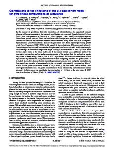
Moreover, design variants with the minimum
Geometric modifications were equally applied on
number of stories (i.e. 3) show a better
all buildings through the parametric variation of
performance, while the extra stories do not seem to
design parameters within the range of values
be so influential. The influence of setbacks is
prescribed by the master plan (i.e. building height),
limited and differentiated. In fact, the north-‐‑south
or those considered representative of possible
setback slightly increases the sDA as it augments
design choices (width and setback). 768 design
the daylight potential on the south-‐‑exposed
variants (#1 to #768) were obtained by combination
external facades, while east-‐‑west setback seems not
of the parameters defining the height and the
to affect sDA.
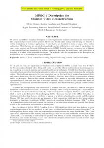
horizontal layout of the building blocks (Figure 1).
minimum acceptable daylight suffiency (IESNA, 2012)
extra stories
horizontal layout width setback
80
sDA300/50%
height stories
buildings
(hereinafter referred to as S, NE and NW blocks because of their relative position in the neighborhood), while taking into account their surrounding context in terms of shading and reflection. For similar reasons, only 32 design variants (#’’1 to #’’32), defined by combination of the maximum and minimum values of each design parameter (Figure 3), were simulated for hourly
stories
three
design variants
extra stories
3 0 17
width
on
#’’
6
setback setback EW NS
Due to the computational cost, the simulations only
40
Figure 2 – Variant-performance plot: spatial Daylight Autonomy
Figure 1 – Schematic of the parametric model
conducted
all blocks
60
20
were
S block NE block NW block
10 3
0 3 0
#’’
design variants
Figure 3 – Parameter-variation plot: set of 32 design variants
illuminances. The metrics were calculated by post-‐‑processing the
Both spatial and temporal false-‐‑color maps are
simulation results in custom MATLAB scripts. The
disposed in a parametric matrix (Figure 4 and
generation of plots and temporal maps was also
Figure 5) confirming that block width is definitely
done in MATLAB, while spatial maps were created
the
through the Rhinoceros/Grasshopper interface.
daylighting.
Only results concerning daylighting are presented
design
3 stories
results, as well as details on the modeling and
variation of design parameters. By analyzing Figure 2 and Figure 3, it can be noted
4 stories
This analysis aims at comparing the trend of performance indicators in relation with the
that block width is by far the most relevant design parameter affecting spatial Daylight Autonomy.
parameter
for
100% 0 10-m block width 17-m block width null N-S setback 3-m N-S setback null N-S setback 3-m N-S setback
provide the widest range of visualizations. All
3.1 Performance Analysis
relevant
occupied hours
in performance and sensitivity analyses, as they
simulation phases, can be found in Peronato (2014).
most
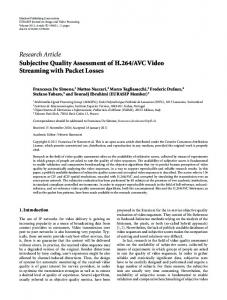
Figure 4 – False-color spatial maps: DA300
Giuseppe Peronato, Emilie Nault, Francesca Cappelletti, Fabio Peron, Marilyne Andersen
In the spatial maps, it can be noted that the number
In addition to what has already been observed (e.g.
of stories is particularly crucial for the daylighting
the relevance of the block width for daylighting),
of the south side of the north-‐‑east block, but a 3-‐‑m
Figure 6 shows that augmenting the building
setback partially compensates the negative effect of
height from 3 to 4 stories has a comparable effect as
the building height, as it can be seen in map #’’10.
adding a 3-‐‑m setback on 4-‐‑story high buildings, as
the curves have similar slopes but opposite angles. surface 100% 0 10-m block width 17-m block width null N-S setback 3-m N-S setback null N-S setback 3-m N-S setback
Conversely, in 3-‐‑story high buildings, the effect of setbacks is much less relevant.
3 stories
3.3 Optimization
The selection of the optimal design solutions was done through the analysis of two decision plots. The decision plot of Figure 7, in which the space of
4 stories
acceptable solutions is defined by the constraints sDA300/50% ≥ 50% and Floor Area Ratio (FAR) ≥ 1.7, allows the selection of a set of six acceptable design variants. The density lower limit is a master plan requirement, while the minimum sDA300/50% was
Figure 5 – False-color temporal maps: tDA300
In the temporal maps, the effect of design parameters is more evident in the time period 12-‐‑ 16 p.m. from April to September for design variants with a 10-‐‑m block width (left half side of
fixed to 50%, as using the minimum daylight sufficiency value (55%) suggested by IESNA (2012) produced an empty solution space.
the matrix), when design variants with 4 stories (second row of the matrix) have a smaller orange area, corresponding to a smaller floor area achieving the 300 lx threshold. However, setbacks
contribute to re-‐‑increasing the dimension of this area, counterbalancing the negative effect of the building height.
3.2 Sensitivity Analysis Because of the large number of design parameters, only a few combinations representing the extreme values of each parameter were considered in this analysis.
Figure 7 – Decision plot: selection of the acceptable solutions
The decision plot of Figure 8 uses the HVAC primary energy (assuming for the heating system a 5% heat losses and, for both heating and cooling
systems, an efficiency of 3.1 and a primary energy no extra stories
conversion factor for electricity of 2.0) and Active
no extra stories
Solar energy production as the two objectives to be respectively minimized and maximized. It should
sDA300/50%
55
be noted that all acceptable solutions, previously
50
selected in Figure 7, show here a low performance
45
for the optimization objectives, while the best
40
solutions, located at the extremes of the axes, do
10 block width 17
3
stories
4
Figure 6 – Parameter-sensitivity plot: sDA300
0
setbacks
3
not achieve the density and/or daylight thresholds. However, by restricting the search for non-‐‑ dominated solutions (as explained in paragraph
A parametric design-based methodology to visualize building performance at the neighborhood scale
2.3.4) to only the acceptable solutions, three design variants (#145, #401 and #657) were selected.
Primary energy (kWh/m2)
This paper has shown a flexible methodology to provide dynamic visualization of the results of
Acceptable Non-dominated
FAR < 1.7 sDA300/50% < 50% FAR < 1.7 and sDA300/50% < 50%
4. Conclusion
building performance simulation for a large number of neighborhood-‐‑scale design variants.
19
The proposed visualizations convey complementary
21
23
the different performance indicators. The false-‐‑color maps, for example, help visualize the suitability of
#145
25
information on the influence of each parameter on
#401
each surface and space for different uses, while, at a
#657
larger scale, sensitivity analysis highlights the
27 130
150 170 190 PV + ST energy production (kWh/m2)
Figure 8 – Decision plot: selection of the optimal solutions
relationship between each design parameter and building performance indicator, so that the designer is more conscious of his/her choices. Finally, the decision plots allow the designer to visualize the
Table 3 – Parameter values of the acceptable solutions
optimal solutions for some given objectives and Extra stories
Stories
Block width
Setback EW
Setback NS
Variant
constraints among the whole set of simulated design variants. However, in the case-‐‑study application, only a few variants resulted acceptable for the chosen constraints, while presenting among the poorest results for the optimization objectives. This proves that optimization is first of all a question of priorities and that the choice to be made by the
#145*
0
0
11
4
0
#146
1
0
11
4
0
#401*
0
0
11
4
1
The main limitations of the methodology are linked
#402
1
0
11
4
1
particular those of interior illuminances, as well as
#657*
0
0
11
4
2
#658
1
0
11
4
2 *non-‐‑dominated
designer (or the decision maker) about which objective(s) to give priority to is fundamental. to the computational cost of simulations, in to the assumptions made for the metrics calculation. Further work should be done to implement the proposed workflow in an interactive design-‐‑support system and to verify its effectiveness in a usability testing study. The support in the choice of
parameters and their range of values through a first
Table 3 shows the geometry characteristics of all
evaluation of simpler metrics would limit the use of
acceptable solutions, including the non-‐‑dominated
time-‐‑expensive simulations. Such platform should
ones. All design variants present 4 stories (the
be finally released as a standalone software or
maximum), an 11-‐‑m block width, which almost
plugin to be used in real design practice.
corresponds to the minimum value (10 m), as well as a null east-‐‑west setback. Moreover, the range of
References
north-‐‑south setbacks is limited to a 0-‐‑to-‐‑1-‐‑m depth,
ASHRAE. 2014. “Annual Heating Load.” ASHRAE Terminology. Accessed November 28, 2014. https://www.ashrae.org/resources-‐‑-‐‑ publications/free-‐‑resources/ashrae-‐‑ terminology Attia, Shady, Liliana Beltrán, André de Herde, and Jan Hensen. 2009. “‘Architect Friendly’: A Comparison of Ten Different Building
while all optimal solutions have a null setback. The designer should hence consider these parameters as particularly important for the performance of the buildings, whereas he/she can have a greater degree of freedom in choosing the extra stories according to other design criteria.
Giuseppe Peronato, Emilie Nault, Francesca Cappelletti, Fabio Peron, Marilyne Andersen
Performance Simulation Tools.” In Proceedings of BS2009, 204–11. Glasgow: IBPSA. Bauart. 2010. Rapport Plan Directeur Localisé Gare-‐‑ Lac. Yverdon-‐‑les-‐‑Bains (CH) Compagnon, R. 2004. “Solar and Daylight Availability in the Urban Fabric.” Energy and Buildings 36 (4): 321–28. doi:10.1016/j.enbuild.2004.01.009. Doelling, Max C. 2014. “Space-‐‑Based Thermal Metrics Mapping for Conceptual Low-‐‑ Enegy Architectural Design.” In Proceedings of BSO2014. London: IBPSA-‐‑ England. Dogan, Timur, Christoph F. Reinhart, and Panagiotis Michalatos. 2012. “Urban Daylight Simulation : Calculating the Daylit Area of Urban Designs.” In Proceedings of SimBuild 2012, 613–20. Madison: IBPSA-‐‑USA. EERE. 2013. “EnergyPlus Engineering Reference : The Reference to EnergyPlus Calculations.” U.S. Department of Energy -‐‑ Energy Efficiency & Renewable Energy (EERE). EN ISO 13790. 2008. “Energy Performance of Buildings -‐‑ Calculation of Energy Use for Space Heating and Cooling (ISO 13790:2008).” CEN. Glaser, Daniel C., and M. Susan Ubbelohde. 2001. “Visualization for Time Dependent Building Simulation.” In Proceedings of BS2001, 423–30. Rio de Janeiro: IBPSA. Haeb, Kathrin, Stephanie Schweitzer, Diana Fernandez Prieto, Eva Hagen, Daniel Engel, Michael Bottinger, and Inga Scheler. 2014. “Visualization of Building Performance Simulation Results: State-‐‑of-‐‑ the-‐‑Art and Future Directions.” In Proceedings of PacificVis 2014, 311–15. IEEE. doi:10.1109/PacificVis.2014.34. IESNA. 2012. IES LM-‐‑83-‐‑12 IES Spatial Daylight Autonomy (sDA) and Annual Sunlight Exposure (ASE). IES LM-‐‑83-‐‑12. IESNA Lighting Measurement. New York. Jakubiec, Alstan, and Christoph F. Reinhart. 2011. “DIVA 2.0: Integrating Daylight and Thermal Simulations Using Rhinoceros 3D, DAYSIM and EnergyPlus.” In Proceedings of BS2011, 2202–9. Sidney: IBPSA. Kleindienst, Siân, and Marilyne Andersen. 2012. “Comprehensive Annual Daylight Design through a Goal-‐‑Based Approach.” Building Research & Information 40 (2): 154–73.
doi:10.1080/09613218.2012.641301. Lagios, Kera, Jeff Niemasz, and Christoph F. Reinhart. 2010. “Animated Building Performance Simulation (ABPS) -‐‑ Linking Rhinoceros/Grasshopper with Radiance/Daysim.” In Proceedings of SimBuild 2010, 321–27. New York: IBPSA-‐‑ USA. Legriel, Julien, Colas Le Guernic, Scotto Cotton, and Oded Maler. 2010. "ʺApproximating the Pareto Front of Multi-‐‑Criteria Optimization Problems."ʺ In Tools and Algorithms for the Construction and Analysis of Systems. Berlin-‐‑Heidelberg: Springer-‐‑ Verlag McNeel. 2013a. Rhinoceros v. 5.0 Windows. Seattle: Robert McNeel & Associates. ———. 2013b. Grasshopper v. 0.9 Windows. Seattle: Robert McNeel & Associates. Peronato, Giuseppe. 2014. “Built Density, Solar Potential and Daylighting: Application of Parametric Studies and Performance Simulation Tools in Urban Design.” Master'ʹs thesis, Venice: Università Iuav di Venezia. Reinhart, Christoph F., Timur Dogan, J. Alstan Jakubiec, Tarek Rakha, and Andrew Sang. 2013. “UMI -‐‑ An Urban Simulation Environment for Building Energy Use, Daylighting and Walkability.” In Proceedings of BS2013. Chambéry: IBPSA. Reinhart, C.F., and O. Walkenhorst. 2001. “Validation of Dynamic RADIANCE-‐‑ Based Daylight Simulations for a Test Office with External Blinds.” Energy and Buildings 33 (7): 683–97. doi:10.1016/S0378-‐‑ 7788(01)00058-‐‑5. Robinson, Darren, Frédéric Haldi, Philippe Leroux, Diane Perez, Adil Rasheed, and Urs Wilke. 2009. “CitySim: Comprehensive Micro-‐‑Simulation of Resource Flows for Sustainable Urban Planning.” In Proceedings of BS2009, 1083–90. Glasgow: IBPSA. Ward-‐‑Larson, Greg, and Rob Shakespeare. 1998. Rendering with Radiance: The Art and Science of Lighting Visualization. San Francisco: Morgan Kaufmann Publishers