These patterns are ideally searched for in massive data sets, which could have origins as diverse as medicine, astronomy, fraud detection, loan granting or.
A Particle Swarm Data Miner Tiago Sousa1 , Arlindo Silva1,2 , and Ana Neves1,2 1
Escola Superior de Tecnologia, Instituto Politecnico de Castelo Branco, Av. do Empres´ ario, 6000 Castelo Branco – Portugal {tsousa,arlindo, dorian}@est.ipcb.pt http://www.est.ipcb.pt 2 Centro de Informatica e Sistemas da Universidade de Coimbra Polo II – Pinhal de Marrocos, 3030 Coimbra Portugal
Abstract. This paper describes the implementation of Data Mining tasks using Particle Swarm Optimisers. The object of our research has been to apply such algorithms to classification rule discovery. Results, concerning accuracy and speed performance, were empirically compared with another evolutionary algorithm, namely a Genetic Algorithm and with J48 - a Java implementation of C4.5. The data sets used for experimental testing have already been widely used and proven reliable for testing other Data Mining algorithms. The obtained results seem to indicate that Particle Swarm Optimisers are competitive with other evolutionary techniques, and could come to be successfully applied to more demanding problem domains.
1
Introduction
Data Mining (DM) and Knowledge Discovery in Databases (KDD) are the most commonly used names to describe the computational efforts meant to process database-stored information, in order to obtain valuable high level knowledge, which must conform to three main requisites: accuracy, comprehensibility and interest for the user [1]. In a nutshell, DM comprehends the actions of (semi) automatically seeking out, identifying, validating and using for prediction, structural patterns in data [2], that might be grouped into five categories: decision trees, classification rules, association rules, clusters and numeric prediction. These patterns are ideally searched for in massive data sets, which could have origins as diverse as medicine, astronomy, fraud detection, loan granting or agriculture. Many approaches, methods and goals have been tried out for DM. Evolutionary approaches such as Genetic Algorithms (GA) and swarm-based approaches like Ant Colonies (AC) [3] have been successfully used. In this paper we propose the use of Particle Swarm Optimisers (PSO) in classification rule discovery. PSO are a new branch in evolutionary algorithms, which were inspired in group dynamics and its synergy and were originated from computer simulations of the coordinated motion in flocks of birds or schools of fish. As these animals Fernando Moura Pires, Salvador Abreu (Eds.): EPIA 2003, LNAI 2902, pp. 43–53, 2003. c Springer-Verlag Berlin Heidelberg 2003 �
44
T. Sousa, A. Silva, and A. Neves
wander through a three-dimensional space, searching for food or evading predators, these algorithms make use of particles moving in an n-dimensional space to search for solutions for an n-variable function optimisation problem. In PSO individuals are called particles and the population is called a swarm [4]. PSO has proved to be competitive with Genetic Algorithms in several tasks, mainly in optimisation areas. Previous research, using PSO for classification tasks [5], has provided results comparing three PSO variants, namely Discrete PSO (DPSO) [6], Linear Decreasing Weight PSO (LDWPSO) [7] and Constricted PSO (CPSO) [8], laying, therefore, the foundations to our present research. In our approach, we opted for the CPSO variant, for it proved to be more qualified when dealing with continuous attributes, which was one of our goals. Temporal complexity was another of our concerns, for without optimisation in this area, expansion to more demanding problems is seriously affected or even made impossible. Following the experimental platform, of the previously mentioned research [5], the same data sets were used, in order to assert whether this approach could offer significant improvements. These data sets were collected mainly from biology and medical science domains. Proving the competitiveness of the PSO Data Miner in these relatively simple domains will lead to successfully applying the same algorithms to problems in the more demanding problem domains mentioned before, like molecular biology and genetics. In section 2 the structure and algorithms used in our work are described in detail. In section 3 we describe the experimental setup and discuss the obtained results which are presented in the section 5. Conclusion and future work are in Section 4.
2
Design Structure and Algorithms
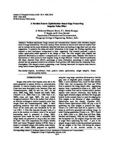
The overall structure of our work was designed to include three nested algorithms; each one fulfils a specific task and is described in details in the following sections.
Fig. 1. Three-nested algorithm application structure
The innermost algorithm, which is the classification rule discovery algorithm, has for its task to find and return the rule, which better classifies the predominant class in a given instance, set. It is here that the PSO algorithm is used.
A Particle Swarm Data Miner
45
The covering algorithm, receives an instance set (the training set), and invokes the classification rule discovery algorithm to reduce this set by removing instances correctly classified by the rule returned by the classification rule discovery algorithm. This process is repeated until a pre-defined number of instances are left to classify in the training set. A sequential rule set is therefore created. The aim of the validation algorithm - the out most algorithm - is not only to determine the accuracy of a rule set returned by the covering algorithm but also to gauge the liability of the whole classifying algorithm - classification rule discovery and covering algorithms altogether. This is achieved by iteratively dividing the initial data set into different test and training sets and computing average indicators, such as accuracy, time spent, rule number per set and attribute tests number per rule. 2.1
Pre-processing Routines – Data Extraction and Normalization
In a pre-processing routine, the original data set is extracted from file, parsed and analyzed. Two data structures are created: a normalized image of the data set and a structure containing metadata information. All attribute values are normalized to the range [0.0, t] with 0.0 < t < 1.0, being t a user pre-defined value, it stands for the indifference threshold where a higher value will trigger the omission of the corresponding attribute test. Three types of attributes were contemplated: nominal, integer and real. Instances containing missing attribute values are discarded. Nominal attributes are normalized assigning to each different attribute value an enumerated index #idx and applying the following equation: idxv × t . (1) #idx idxv is the index of the attribute value v and #idx the total number of different attribute values. Both integer and real types are normalized with equation 2. vnorm =
(v − vmin ) × t . (2) vmax − vmin vmin and vmax are the lower and higher attribute values found for this attribute. A state attribute is assigned to each instance. Manipulating this state value, it is very easy and computationally efficient, to divide the data set into training and test sets and to (pseudo-) remove instances. This attribute takes the following values: TEST, TRAIN and REMOVED. vnorm =
2.2
Rule Representation
Classification rules are no more than conditional clauses, involving two parts: the antecedent and the consequent. The former is a conjunction of logical tests, and the latter gives the class that applies to instances covered by this rule. These rules take the following format:
46
T. Sousa, A. Silva, and A. Neves
IF attribute_a=value_1 AND attribute_b=value_2 ... AND attribute_n=value_i THEN class_x In rule classifier systems there are two distinct approaches to individual or particle representation: the Michigan and the Pittsburgh approaches [9]. In the Michigan approach each individual encodes a single rule, whereas in the Pittsburgh approach each individual encodes a set of rules. In our work, we follow the Michigan approach and rules are encoded as a floating-point array; each attribute is represented by either one or two elements on the array, according to its type. Nominal attributes are assigned with one element on the array and attribute-matching tests are defined as follows: true if �vr × #idx� = �vi × #idx� m(vr , vi ) = (3) f alse otherwise. Being t the indifference threshold value, vr the attribute value stored in the rule for testing and vi the instance value stored in the normalized image of the data set. Integer and real attributes are assigned with an extra element in the array in order to implement a value range instead of a single value, true m(vr1 , vr2 , vi ) =
if vr1 ≥ t or (vr1 − vr2 ) ≤ vi or (vr1 + vr2 ) ≥ vi
f alse otherwise.
(4) vr1 can be seen as the center and vr1 as a neighbourhood radius, inside which matching will occur. 2.3
Classification Rule Discovery Algorithm – Particle Swarm Optimisation
As previously mentioned, the rule discovery process is achieved through a PSO algorithm. PSO are inspired in the intelligent behavior of beings as part of an experience sharing community as opposed to an isolated individual reactive response to the environment. The Adaptive Culture Model [6], which is PSO’s framing theory, states that the process of cultural adaptation is rooted into three principles: evaluate, compare and imitate. Evaluation is the capacity to qualify environmental stimuli and the sine qua non condition to social learning. Evaluation itself is both useless and impossible without the ability to compare; all of our metrics are but a comparison to a wellknown unit and a single value becomes pointless without the values of its peers. At last, imitation is the rawest form of experience sharing from the receiver’s
A Particle Swarm Data Miner
47
standpoint; it involves not only observation but also the realization of purpose and timing adequacy. In PSO algorithms, a particle decides where to move next, considering its own experience, which is the memory of its best past position, and the experience of its most successful neighbour. There may be different concepts and values for neighbourhood; it can be seen as spatial neighbourhood where it is determined by the Euclidean distance between the positions of two particles, or as a sociometric neighbourhood (e.g.: the index position in the storing array). The latter is the most commonly used for two main motives: if space coordinates were to represent mental abilities or skills, two very similar individuals may never come to meet in their lifetime, as to elements of the same family, which may differ significantly from each other, but still, they will always be neighbours. The other motive is related with the computational effort required to process the Euclidean distance, when faced with large number of particles or dimensions - in each iteration, the distance between every two particles would have to be calculated and for each particle the nearest k neighbours would have to be sorted out. The number of neighbours (k) usually considered is either k = 2 or k = all. Although some actions differ from one variant of PSO to the other, the pseudo-code for PSO is as follows: Initiate_Swarm() Loop For p=1 to number of particles Evaluate(p) Update_past_experience(p) Update_neighbourhood_best(p,k) For d=1 to number of Dimensions Move(p,d) Until Criterion . Inevitably, with more or less iterations, the swarm converges to an optimum (possibly just a local one). In our implementation, the criterion used to trigger the ending of the loop is the realization all particles in the swarm are within a user-defined distance from the best particle in the swarm. In order to manipulate equivalent threshold distances, considering that distance ranges will differ accordingly to the dimension number, the distance formula used is the normalized Euclidean distance � d(p1 , p2 ) =
n � i=1
(pi1 − pi2 )2 √
d.
(5)
p1 and p2 are particles and d the dimension number, pin stands for the ith coordinate value of particle pn . As each dimension coordinate is bounded to the interval [0.0, 1.0] the maximum value for (pi1 − pi2 ) is 1.0, which when squared
48
T. Sousa, A. Silva, and A. Neves
remains 1.0, therefore to normalize a distance, all that is needed is to divide it √ by d. The output of this algorithm is the best point in the hyperspace the swarm visited - and in this case, converged to. There are several variants of PSO, typically differing in the representation: Discrete or Continuous PSO[6]; in the mechanism used to avoid spatial explosion of the swarm and guaranteeing convergence: Linear Decreasing Weight[7] or Constricted PSO[8]; or in the mechanism used to avoid premature convergence to local optima: Predator Prey[10] or Collision Avoiding Swarms[11]. The variant used in our work was the Constricted PSO (CPSO). There is a need to maintain and update the particle’s previous best position (Pid ) and the best position in the neighbourhood (Pgd ). There is also a velocity (Vid ) associated with each dimension, which is an increment to be made, in each iteration, to the dimension associated (equation 6), thus making the particle change its position in the search space. vid (t) = χ(vid (t − 1) + ϕ1id (Pid − xid (t − 1)) + ϕ2id (Pgd − xid (t − 1)))
(6) xid (t) = xid (t) + vid (t)
ϕ1 and ϕ2 are random weights defined by an upper limit, χ is a constriction coefficient [8] set to 0.73. The general effect of equation 6 is that each particle oscillates in the search space between its previous best position and the best position of its best neighbour, hopefully finding new best points during its trajectory. If the particle’s velocity were allowed to change without bounds the swarm would never converge to an optimum, since particles oscillations would grow larger. The changes in velocity are therefore limited by χ - the constriction coefficient - forcing the swarm to converge. The value for this parameter and for the upper limits on ϕ1 and ϕ2 can be chosen to guarantee convergence [8]. In our experiments χ was set o 0.73 while ϕ1 and ϕ2 upper limits were set to 2.05. 2.4
Rule Evaluation – Establishing Points of Reference
Rules must be evaluated during the training process in order to establish points of reference for the training algorithm: best particle positioning. The rule evaluation function must not only consider instances correctly classified but also the ones left to classify and the wrongly classified ones. The formula used to evaluate a rule and therefore set its quality is expressed in equation 7 [9]: TP N if 0.0 ≤ xi ≤ 1.0, ∀i ∈ d T P +F N × T NT+F P Q(X) = (7) −1.0 otherwise Where:
A Particle Swarm Data Miner
49
• T P - True Positives = number of instances covered by the rule that are correctly classified, i.e., its class matches the training target class. • F P - False Positives = number of instances covered by the rule that are wrongly classified, i.e., its class differs from the training target class. • T N - True Negatives = number of instances not covered by the rule, whose class differs from the training target class. • F N - False Negatives = number of instances not covered by the rule, whose class matches the training target class. This formula penalizes a particle, which as moved out of legal values, assigning it with negative value (−1.0), forcing it to return to the search space. 2.5
Covering Algorithm – Rule Set Construction
The covering algorithm is basically a divide-and-conquer technique. Being given a instance training set, it runs the rule discovery algorithm in order to obtain the highest quality rule for the predominant class in the training set. Correctly classified instances are then removed from the training set and the rule discovery algorithm is run once more. Iteratively a sequential rule set is built, and the covering algorithm runs until only a pre-defined number of instances are left to classify. This threshold criteria value is user-defined as a percentage and it is typically set to 10%. A default rule, to capture and classify instances not classified by the previous rules is added to the rule set. Containing no attribute tests and predicting the same class as the one predominant in the remaining instances, this rule takes the form: IF true THEN class_x. 2.6
Validation Algorithm – Rule Set and Overall Evaluation
The purpose of the validation algorithm is to statistically evaluate the accuracy of the rule set obtained by the covering algorithm. This is done using a method known as tenfold cross validation [2]. The tenfold cross validation consists in dividing the data set into ten equal partitions and iteratively using one of this sets as a test set and the remaining nine as training sets. In the end ten different rule sets are obtained and average indicators, such as accuracy, time spent, rule number per set and attribute tests number per rule are computed. Several other numbers for partitioning have been tried out, but theoretical research [2] has shown that ten offers the best estimate of errors. Rule set accuracy is evaluated and presented as the percentage of instances in the test set correctly classified. An instance is considered correctly classified, when the first rule in the rule set, whose antecedent matches this instance and the consequent (predicted class) matches this instance’s class.
50
2.7
T. Sousa, A. Silva, and A. Neves
Post-processing Routines – Rule Pruning and Rule Set Cleaning
Recall that high level knowledge extracted from databases must conform to three main requisites: accuracy, comprehensibility and interested for the user [1]. In classification rule discovery problems, the number of attribute tests per rule and the number of rules per set is a major contributor for the comprehensibility of the obtained results - fewer attribute tests and rules eases comprehensibility. After a rule is returned from the classification rule discovery algorithm it goes through a pruning process in order to remove unnecessary attribute tests. This is done by iteratively removing each attribute test whenever the newly obtained rule has the same or higher quality value than the original rule. Just after the covering algorithm returns a rule set, another post-processing routine is used: rule set cleaning, where rules that will never be applied are removed from the rule set. As rules in the rule set are applied sequentially, in this routine, rules are removed from the rule set if: • There is a previous rule in the rule set that has a subset of the rule’s attribute tests. • If it predicts the same class as the default rule and is located just before it. So in the example below, rules number 2 and 3 will be removed and the rule set will be reduced to the first and last rules: Rule #1 If attribute_a = x_a Then class=c_1 Rule #2 If attribute_a = x_a and attribute_b=x_b Then class=c_2 Rule #3 If attribute_c = x_c Then class=c_3 Rule #4 - Default Rule If TRUE Then class=c_3.
3
Experimental Results
Experimental results are presented and discussed in this section. To maintain a fair experimental platform with [5] the same data sources were used: two regarding Breast-Cancer diagnosis, and the other, animal classification. These are standard benchmark problems which can easily be used to compare results with a vast number of other implemented algorithms thus allowing us to compare the effectiveness of our PSO based algorithms, not only with the other algorithms implemented by us, but also with previous results obtained from the literature.
A Particle Swarm Data Miner
51
To help benchmarking the evolutionary algorithms implemented, results were also obtained with a well-known standard tree induction algorithm, J48, a Java implementation of C4.5. 3.1
Experimental Setup
In [5] attribute testing, indifference was implemented with an extra bit (particles were coded in binary strings), as a result indifference probability occurrence will vary accordingly to the attribute assigned bit number and its range of possible values, in the interval ]1/2, 3/4]. In our work a user defined threshold level maintains attribute-testing indifference, therefore different values for this threshold were tested in order to evaluate its influence. The data sources used were obtained from the Department of Computer Science, University of Waikato, Hamilton, New Zealand[13], and Information and Computer Science, University of California [14]. In section 5 we present the experimental results obtained. Accuracy values are in percentage of success, and are obtained by averaging ten-fold accuracy results. The swarms were set to 25 particles, convergence radius to 0.1 and minimum uncovered instances to 10%. 3 data sets were used: Zoo, Wisconsin-Breast-Cancer and Breast-Cancer. Zoo is a data set that classifies animals according to their characteristics. WisconsinBreast-Cancer and Breast-Cancer are real data sets that classify if the tumour was malignant/benign and if recurrence of events did happen. 3.2
Discussion
Results obtained clearly state the competitiveness of CPSO with industrial tree induction algorithms like J48, a Java implementation of C4.5. Trees obtained with J48 are easily converted to rules - each path from the root to a leaf stands for a rule. There is a clear relation between indifference threshold level value and accuracy results: best results were obtained with lower values for indifference threshold level. Rule pruning and rule set cleaning routines indicate as expected to be strong contributors comprehensibility. Both CPSO versions did surpass J48 in the Wisconsin-Breast-Cancer relation. Regarding accuracy, all tested algorithms seem to be equivalent. Nevertheless, temporal complexity of both CPSO versions are still much more demanding than J48, possibly due to the nature of the algorithm and processing involved.
4
Conclusions and Future Work
We proposed to improve one of the PSO variants investigated in [5] and evaluate the possible influence of the indifference threshold values. We implemented
52
T. Sousa, A. Silva, and A. Neves
and compared this variant with the corresponding one in [5] and J48, in some benchmark data. From the results, we can conclude that PSO can obtain competitive results against J48 in the data sets used, although there is some increase in the computational effort needed. We can also conclude, that lower values for indifference threshold offer the best accuracy results. Both post-processing routines: rule pruning and rule set cleaning, contribute greatly to comprehensibility. Directions for future work include an empirical analysis of the influence of indifference threshold with exploration and exploitation. Applying this tool to more demanding data sources, containing continuous attributes. We hope that a more focused and better-tuned PSO based algorithm will surpass the results obtained with this approach, making PSO a real competitive technique in DM.
References 1. Fayyad, U.M., Piatetsky-Shapiro, G. and Smyth, P.: From Data Mining to Knowledge Discovery: an Overview. Advances in Knowledge Discovery and Data Mining, 1–34. AAAI/MIT, Cambridge (1996). 2. Witten, Ian H. and Frank, E.: Data Mining – Practical Machine Learning Tools and Techniques with Java Implementations. Morgan Kauffmann (1999). 3. Parpinelli, R., Lopes, H. and Freitas, A.: An Ant Colony Algorithm for Classification Rule Discovery. Idea Group (2002). 4. Kennedy, J. and Eberhart, R. C.: Particle Swarm Optimisation. Proc. IEEE, International Conference on Neural Networks. Piscataway (1995). 5. Sousa, T., Silva, A. and Neves, A.: Particle Swarm Optimisation as a New Tool for Data Mining. International Parallel and Distributed Processing Symposium (IPDPS). Nice, France, (2003). 6. J. Kennedy, Eberhart, R. C.: Swarm Intelligence Morgan Kauffman, (2001). 7. Shi, Y. and Eberhart, R. C.: Empirical Study of Particle Swarm Optimisation. Proceedings of the 1999 Congress of Evolutionary Computation. Piscatay (1999). 8. Clerc, M. and Kennedy, J.: The Particle Swarm-Explosion, Stability and Convergence in a Multidimensional Complex Space. IEEE Transactions on Evolutionary Computation, Vol. 6 No.1. (2002). 9. Lopes, H.S., Coutinho, M. S. and W. C.: An Evolutionary Approach to Simulate Cognitive Feedback Learning in Medical Domain. Genetic Algorithms and Fuzzy Logic Systems: Soft Computing Perspectives. ISBN 981-02-2423-0, World Scientific Singapore, (1997). 10. Silva, A., Neves, A. and Costa E.: Chasing the Swarm: A Predator Prey Approach to Function Optimisation. Proc. of MENDEL2002 – 8th Interna-tional Conference on Soft Computing. Brno, Czech Republic, (2002). 11. Blackwell, T. and Bentley, P. J.: Don’t Push Me! Collision-Avoiding Swarms. Proc. of the Congress on Evolutionary Computation, (2002). 12. Freitas, A.: A survey of evolutionary algorithms for data mining and knowledge discovery. Ghosh, A.; Tsutsui, S. (Eds.) Advances in evolutionary computation. Springer-Verlag, (2001). 13. ftp://ftp.cs.waikato.ac.nz/pub/ml/datasets-UCI.jar 14. http://www.ics.uci.edu/ cmerz/mldb.tar.Z
A Particle Swarm Data Miner
5
53
Appendix: Results
Table 1. Relation Zoo Indifference Pruning Rule Set Cleaning Accuracy Time Spent Number of Rules Tests per Rule
J48 — — — 92.07 0.09 13 5
CPSO[5] 0.5 - 0.7 y y 76.67 11.75 7 2
0.1 n n 89.00 11.00 6 6
0.5 n n 86.33 16.00 10 31
CPSO 0.7 n n 80.33 48.00 181 1224
0.1 y y 89.04 17.36 6 5
0.5 y y 77.00 13.01 6 4
0.7 y y 46.67 3.35 5 4
0.1 y y 76.66 28.13 6 5
0.5 y y 75.18 13.19 6 5
0.7 y y 73.33 17.81 6 5
0.5 y y 91.81 67.16 7 4
0.7 y y 76.61 18.05 5 4
Table 2. Relation Breast-Cancer Indifference Pruning Rule Set Cleaning Accuracy Time Spent Number of Rules Tests per Rule
J48 — — — 72.92 0.03 4 2
CPSO[5] 0.5 - 0.7 y y 76.42 7.04 5 2
0.1 n n 75.80 26.45 6 5
0.5 n n 74.56 11.54 6 5
CPSO 0.7 n n 74.44 25.73 7 8
Table 3. Relation Winsconsin-Breast-Cancer Indifference Pruning Rule Set Cleaning Accuracy Time Spent Number of Rules Tests per Rule
J48 — — — 92.82 0.02 55 2
CPSO[5] 0.5 - 0.7 y y 93.92 17.34 7 1
0.1 n n 92.89 117.42 7 4
0.5 n n 90.63 87.84 8 7
CPSO 0.7 n n 92.00 114.27 40 122
0.1 y y 92.84 85.01 7 4