Given the pass/fail information, the timing validation is to determine if the behavior is consistent with the timing model used in the pre-silicon design. Without loss.
A Path-Based Methodology for Post-Silicon Timing Validation Leonard Lee1 , Li-C. Wang1 , T. M. Mak2 , and Kwang-Ting Cheng1 1 Department of ECE, UC-Santa Barbara 2 Intel Corporation, Santa Clara, CA Abstract
power noise, crosstalk, thermal effects, etc. [1, 2, 3]. These effects are hard to predict and model deterministically. For these effects, traditional discrete-value timing models become ineffective. Statistical timing analysis and timing simulation approaches are among the many that promise to better handle these deep submicron (DSM) timing effects [4]-[11]. However, even with a statistical timing approach, it is hard to ensure that a timing model can accurately capture all aspects of DSM timing effects. As the complexity of timing models continues to increase, their accuracy and correct usage in design analysis may come into question. Today, it has become increasingly difficult for a timing signoff tool to guarantee silicon results. This means that inevitably, some of the non-defect-related timing problems have to be resolved in the post-silicon stage. In order to analyze the timing problems in the post-silicon stage, we require a novel methodology to perform statistical inference (or reasoning) based on the observed timing behavior on the silicon. The difficulty of developing such a post-silicon timing validation methodology lies in the constraint of lacking internal cell delay information in the analysis. This is why such information has to be obtained through inference and reasoning based on the observed delays on the silicon. Therefore, in this work we present a novel approach to derive post-silicon path ranking based on inference from observed timing behavior. This path ranking serves as the basis in our validation methodology. Our path ranking methodology consists of two inference approaches: ranking optimization and path filtering. In ranking optimization, we formulate the problem as a minimization problem. Given a set of paths U and the observed timing behavior on a set of patterns PA, the objective is to find delay assignments to all paths in U in order to minimize an estimated error function. The error function characterizes how feasible the delay assignments are, based on the observed timing behavior. In path filtering, our objective is to utilize statistical learning techniques to correlate logic path sensitization to pattern delays as that outlined in [12]. Then, we derive a statistically important subset of paths that is sufficient to explain the observed behavior. The post-silicon path ranking is compared to the pre-silicon path ranking in order to determine if the timing model is consistent with the observed behavior. To derive a pre-silicon path ranking, we can simply use any timing analysis tool capable of calculating path delays. In this work, we use a false-path-aware statistical timing analysis tool [7]. To obtain sample chip behavior for the experiments, this work utilizes a statistical timing simulator developed in the past. The prototype simulator was introduced in [15] and was later used to conduct research in [16]-[17]. In our experiments, we use the statistical timing analyzer as the pre-silicon timing tool to derive path
This paper presents a novel path-based methodology for postsilicon timing validation. In timing validation, the objective is to decide if the timing behavior observed from the silicon is consistent with that predicted by the timing model. At the core of our path-based methodology, we propose a framework to obtain the post-silicon path ranking from observing silicon timing behavior. Then, the consistency is determined by comparing the post-silicon path ranking and the pre-silicon path ranking calculated based on the timing model. Our post-silicon ranking methodology consists of two approaches: ranking optimization and path filtering. We discuss the applications of both approaches and their impacts on the path ranking results. For experiments, we utilize a statistical timing simulator that was developed in the past to derive chip samples and we demonstrate the feasibility of our methodology using benchmark circuits.
1. Introduction Given a set of patterns PA and a set of test chips, by applying PA on these chips with various clock frequencies, we can obtain the pass/fail behavior of the chips. Given the pass/fail information, the timing validation is to determine if the behavior is consistent with the timing model used in the pre-silicon design. Without loss of generality, we may assume that by applying as many different clocks as we want, it is possible to determine the delay of a pattern on a given test chip. This delay can be the shortest clock period where the chip does not fail with the pattern. The application of many different clocks for all patterns can be an expensive process. However, this can be done based on a small number of test chips. Moreover, applying tests with multiple clock frequencies is commonly required for speed binning. Therefore, having estimated the delays of all patterns, it remains to be an interesting question to ask if the observed timing behavior is consistent with that predicted by the timing model, and if not, what the most representative subset of paths should be for us to debug the problem. Historically, post-silicon timing validation receives less attention than delay testing. In delay testing, we assume that timing errors are mostly due to manufacturing defects. Hence, if we signoff a chip design with the target of k MHz, then without manufacturing defects, we would expect that most of the real chips should behave as fast as k MHz. This means that at the stage of testing, our objective would be to screen out bad chips due to manufacturing defects. However, with the advances to nanometer technologies, this assumption is hardly true. In the deep sub-micron (DSM) domain, circuit timing reflects many important sources of effects such as process variations,
0-7803-8702-3/04/$20.00 ©2004 IEEE.
713
delays. To obtain post-silicon timing behavior, we use the timing simulator to simulate the application of tests on a number of sample chips. To study the proposed methodology, we may use the same timing model or two different timing models in the analyzer and the simulator. The rest of the paper is organized as the following. In Section 2 we define the problem of post-silicon path ranking and point out key considerations. Section 3 describes the key tools used in our experiments. In Section 4, we discuss the ranking optimization problem. Section 5 discusses the path filtering approach based on statistical learning and the impact of producing more patterns for select paths. Section 6 summarizes additional experimental results. Section 7 concludes the paper and discusses future research.
Through functional sensitization analysis, suppose we can associate subsets of paths S = {U1 , . . . ,Un } to the patterns x1 , . . . , xn , respectively. Then, the problem of path ranking becomes how to derive path delays from the given (PA, Dmean , S). For any path p ∈ U but p �∈ Ui for any i (1 ≤ i ≤ n), we simply ignore this path because no delay information can be derived. An interesting problem related to the path ranking is to establish the mapping f such that f (PA, S) ≈ Dmean . That is, ∀xi ∈ PA,Ui ∈ S, f (Ui ) can be used to predict the value of Dmean (xi ). The mapping f can be non-linear. The author in [12] proposed a methodology to solve a different but similar mapping problem. Define the critical probability crti of a pattern xi on the N test chips as the percentage of the chips failing a given test clock clk. The methodology derives a mapping f � such that ∀xi ∈ PA,Ui ∈ S, f � (Ui ) ≈ crti . The methodology utilizes a statistical learning technique called Support Vector Machine (SVM) [18][19]. Essentially, each (Ui , crti ) can be seen as a training sample point in a learning problem and SVM can be used to derive a statistical learned model from all sample points. If the mapping f can be established, then f can be used to extract statistically important paths. This is equivalent to asking the following question. Given the original path set U, can we find a minimal-size subset Umin of U such that the learned mapping fmin based on the smaller subset Umin is as effective as the original f based on U? Then, the paths in Umin can be seen as the statistically important paths. In statistical learning, this problem of finding Umin is called the feature selection problem [21][22]. We note that deriving the statistically important paths does not reveal any information about the ranking of paths. For path ranking, the prior learning-based methodology alone is not sufficient. In general, the path ranking is not an easy problem to be solved (as we will see in the discussion in later sections). Hence, we propose two complementary approaches for solving the problem. In ranking optimization, we try to derive a path ranking based on the given information (PA, Dmean , S). In path filtering, we try to filter out statistically unimportant paths based on a SVM-learningbased methodology. In other words, since ranking optimization may not solve the path ranking problem completely, we may need a path filtering approach to identify potential paths whose ranks cannot be correctly established by ranking optimization.
2. The Path Ranking Problem Suppose that we are given a set of patterns PA = {x1 , . . . , xn } and N = {t1 , . . . ,tN } test chips. By applying xi on t j with various clocks, we assume that we can obtain the worst-case delay di j . Let the observed timing profile be T = {di j |1 ≤ i ≤ n, 1 ≤ j ≤ N}. Let U = {p1 , . . . , pm } be a given path set. Given (PA, T,U), the problem of path ranking is to derive the delays of paths in U in order to obtain a feasible ordering among them. Since there are N test chips, for each pattern xi we have N delay values di1 , . . . , diN which may be different. These delay values form a delay distribution for xi . In order to define a path ranking, we need to define how to order two patterns based on their delay distributions. To simplify the analysis, this work utilizes the mean delays to define the ranking. The mean delay of xi is simply iN . Dmean (xi ) = di1 +···+d N Given the mean pattern delays, the path ranking problem can be solved by answering the question of how to derive path delays from these pattern delays. The inference from pattern delays to path delays would be trivial if for each pattern xi , there is at most one path in U such that this path has a chance to decide the delay of xi . If the path ranking problem is given with a (PA,U) pair with this property, then the solution is straightforward. In general, a pattern may be associated with many paths in U, which all have a chance to decide the delay of the pattern (to be the speed-limiting path). This is especially true if the patterns are based on transition faults instead of path delay faults or if the patterns are functional patterns and the paths spread in different functional blocks. Even with path delay fault patterns, due to cosensitization, timing hazards, and fortuitous sensitization, more than one path can be affecting the delay of a pattern. In this case, the path ranking problem becomes interesting. In order to determine if a path has a chance to decide the delay of a pattern, we can utilize logic simulation to analyze path sensitization. For example, if a path is functionally sensitized by a pattern, then there is a chance that the pattern delay is determined by the path delay. We note that a path is functionally sensitized by a pattern if (1) there are transitions on all on-inputs of the path, and (2) all side-inputs of the path have non-controlling values from the second vector of the given pattern [25] if the corresponding oninputs also have non-controlling values from the second vector. Note that functional sensitization is not the only way to sensitize a path [25]. Moreover, if a path has a timing hazard [23], we can use the same logical conditions to decide if the hazard has a chance to affect the path output delay and consequently, the pattern delay.
3. Tools and Methodologies For Experiments Throughout the work, we use a statistical static timing analyzer (SSTA) [7] to obtain the pre-silicon path ranking and a statistical timing simulator (STS) to produce sample chip results for the postsilicon path ranking. Given a cut-off threshold clock, the SSTA tool can output the set of paths whose critical probabilities (based on the clock) are not zero. We use this set as the initial path set U. To assess the effectiveness of our post-silicon path ranking methodology, the SSTA and STS will employ the same timing model. Hence, if our post-silicon path ranking method is perfect, the two rankings should be close to identical. To demonstrate the usefulness of the post-silicon ranking, we will intentionally change the timing model in SSTA so that it does not match the model used in STS. For example, we can alter the SSTA timing model by using only the rising pin-to-pin delays instead of both the rising and falling pin-to-pin delays. This will increase the delays of many paths, as rising delays tend to be larger.
714
estimated error Err. Definition 4.2 translates the problem of searching for a feasible delay assignment in an ill-defined space to a problem of searching for a weight assignment in a well-defined space. Such an approach is quite common in statistical analysis. In searching for a feasible model, we often need to provide hypothetical constraints to restrict the search in order to make the problem solvable with reasonable computational resources.
Given the initial set of paths, we use a SAT-based path oriented ATPG tool [20] to produce non-robust patterns for the paths, one pattern for each path. The unnecessary primary inputs are filled randomly with 0 or 1s. Since not all false paths can be eliminated by SSTA, the ATPG may fail to produce a pattern for some paths. In this case, we just ignore the result. However, these paths would still be kept in the initial path set. Since the main objective here is to study the feasibility of the proposed path-based methodology, this paper does not consider other types of pattern sets. Given the pattern set PA and the path set U, for each pattern xi we need to produce the sensitized path subset Ui as described in Section 2. We wrote a simple logic sensitization tool Path-Sen for this purpose. For post-silicon analysis, this is our only view of the inner workings of a circuit, which should be readily available from the design process leading to first silicon. For our experiments, we assume that we have a gate level representation of a circuit that can be used to extract sensitization information. Our statistical timing model assumes pin-to-pin delay random variables. The timing model is cell-based, and interconnects’ delays can be included for consideration. For experimental purposes, the random delay distributions were obtained using a MonteCarlo-based SPICE simulator (ELDO) [26]. We extracted the cells’ pin-to-pin delay distributions from a 0.25µm, 2.5V CMOS technology.
4.1. A simple greedy search heuristic Definition 4.2 defines a minimization problem that, similar to most of the problems in practice, is likely to be as hard as an NP-complete problem or beyond. In this work, we do not try to develop an optimal algorithm for solving the problem. Instead, we provide a simple greedy heuristic. The following depicts the heuristic. 1. Let W = {1, . . . , 1}. 2. Let ρ > 1 be a given rate. For example, the default value of ρ can be 10. 3. Repeat the following steps k times. (a) Based on the current weight assignment W , calculate the delay assignment Dassign ← Dave . (b) Calculate the estimated error erri for every pattern xi and then, the total error Err.
4. Path Ranking Optimization
(c) Find the five patterns whose estimated errors are among the largest. Randomly pick one from these five patterns. Let this pattern be x j .
Given (PA, Dmean , S), our objective is to derive a feasible delay assignment Dassign = {d1 , . . . , dm } to paths {p1 , . . . , pm }, which are most consistent with the observed timing behavior Dmean . This ”feasibility” can be measured as the following. Suppose for a pattern xi , Ui = {pi1 , . . . , pik }, i.e. the pattern functionally sensitizes these k paths. The delay assignment Dassign gives the delays {di1 , . . . , dik } for all paths in Ui . Based on these delays and Ui , fixed-delay simulation can calculate the longest delay value from Ui . Let this delay be denoted as Dassign (xi ). We note that Dassign (xi ) is not necessarily = max(di1 , . . . , dik ). For example, if two paths merge at a gate where both have the transition from the non-controlling value to the controlling value of the gate, then the minimum delay of the two dominates. Conversely, if both have the transition from the controlling value to the noncontrolling value, then the maximum delay of the two dominates. Definition 4.1 (Estimated Error) Given the two delays Dmean (xi ) and Dassign (xi ) for pattern xi , we define the estimated error erri = (Dmean (xi ) − Dassign (xi ))2 . The total estimated error Err from a delay assignment Dassign is Σni=1 (erri ). We use the total estimated error Err to evaluate the feasibility of a delay assignment Dassign to the paths. To facilitate the search for a feasible delay assignment, we assume the following constraint. Let pi be a path sensitized by j patterns xi1 , . . . , xi j . We assume that the delay of pi is equal w D
(x )+···+w D
(d) Update the weight of x j as w j ← w j + ρ × err j . 4. Output the delay assignment whose total estimated error is the minimum during the k iterations. The reasoning behind the above heuristic is the following. In each iteration, we identify a pattern with a large error value. To fix this large error value, we would increase the pattern’s weight so that this pattern delay has dominating effect in the calculation of the weighted average. This would result in assigning delay values, which are close to the pattern delay, to all paths sensitized by this pattern and consequently, reduce the error for this pattern. However, we note that this weight change may increase the errors of other patterns. The reason why we pick five patterns and randomly choose one, instead of simply choosing the one with the largest error, is to avoid the search falling into a local loop. For example, two patterns xi , x j may have estimated errors much larger than the others. When we fix the weight for xi , the error of pattern x j increases and appears to be the largest. Then, we fix the weight for x j , and the error of xi increases and appears to be the largest. In this situation, simply focusing on the pattern with the largest estimated error will not be effective.
(x )
to Dave (pi ) = i1 mean wi1i1 +···+wii jj mean i j , i.e. the weighted average of all the pattern delays. Hence, given a weight assignment W = {w1 , . . . , wn } for patterns PA = {x1 , . . . , xn }, we can calculate the weighted average Dave (pi ) for each path pi . Then, this weighted average will serve as one solution for Dassign . Definition 4.2 (Ranking Optimization) Given (PA, Dmean , S), the problem of ranking optimization is to find a weight assignment W , resulting in a delay assignment Dassign to minimize the total
4.2. Initial experiments to illustrate the heuristic To illustrate the above heuristic, in this section we present experimental results based on the ISCAS85 benchmark c880. By selecting the SSTA clock properly, we were able to construct a U172 path set with 172 paths. Then, we produce a pattern for each path. We first sort these paths according to their mean delays calculated by SSTA. Then, we select 86 paths (U86 ) from the
715
estimated error tracks the true error well, i.e. they follow similar trends. Hence, this justifies using the estimated error in our heuristic to guide the search process. In practice, we do not know the true error because we cannot assume that the ranking from the SSTA should be identical to the post-silicon ranking. Hence, we could not use the true error to guide the search in the heuristic. This is why we need to use the estimated error. (2) To obtain a delay assignment with minimal error, there is no need to run a large number of iterations. Usually, the error value drops quickly during the first few iterations and then does not change significantly for the remaining iterations. In this experiments, about 50 iterations are sufficient to obtain a good result.
172 paths by selecting every other path according to the ranked order. Then, from the 86 paths, we select 43 paths (U43 ) by selecting every other path again. For each path set, we apply the patterns from those paths in the set only. Call these three pattern sets PA172 , PA86 , PA43 , respectively. We first focus on U86 . Based on the path set and the pattern set PA86 , we use the path sensitization checking tool Path-Sen to construct the sensitization profile S86 = {U1 , . . . ,U86 }. We use SSTA to derive a path ranking Rssta for paths in U86 and use STS and the above heuristic to derive a post-silicon path ranking R post . In STS, the number of simulated samples is 200. We note that in our path ranking, a small number means that the path has a larger delay. Hence, we call a path with a small ranking number as a high ranking path, and vice versa. Given the two rankings Rssta and R post , we can calculate the true ranking error by comparing these two. For a path p, the true error of the path is calculated as errtrue (p) = 12 (Rssta (p) − R post (p))2 . Figure 1 illustrates the calculation of the true error.
4.3. Path ranking results Given the two rankings Rssta and R post , we will plot R post against Rssta to evaluate how these two correlate. Figure 3 shows the results where SSTA and STS employ the same timing model. Figure 3-(a) shows the correlation plot by selecting the delay assignment giving the minimum estimated error from the 200 iterations. Figure 3-(b) shows the result by selecting the delay assignment giving the minimum true error. As it can be seen, both plots look similar.
1/2(a−b) (a, a)
| a−b |
SSTA ranking
Figure 1: The true error in path ranking. In the ideal case (where SSTA and STS have exactly the same timing model), the two rankings should be identical as denoted as the line ”x = y” in the figure. For a path with the � two ranks denoted
SSTA ranking
1 2 2 (a − b) .
(a)
SSTA ranking
(a)
(b)
Figure 3: The results of path ranking based on estimated error vs. true error. In contrast, Figure 4 shows the results where SSTA and STS employ different timing models. In Figure 4-(a), each pin-to-pin falling delay in the cell library is ignored and replaced by its corresponding pin-to-pin rising delay. In Figure 4-(b), we use only the falling delays and ignore the rising delays. Unlike what is shown in Figure 3-(a), the SSTA path rankings do not correlate well to the post-silicon path rankings in Figure 4.
Post-silicon ranking
True Error
Estimated Error
Hence, as (a, b), its distance from the x = y line is the true error is measured by the distance from the ideal answer. We calculate the true total error as Errtrue = Σm i=1 errtrue (pi ). The total estimated error Err is defined based on patterns (please refer to Definition 4.1) and the true error Errtrue is calculated based on path ranking comparison. It is interesting to compare these two errors during the iterations of the proposed heuristic. Figure 2 compares the two errors in the case of c880. The number of iterations is 200.
Iteration
Post-silicon ranking (from true error)
| b − a | (a, b)
Post-silicon ranking
(b, b)
Post-silicon ranking (from estimated error)
Post−silicon ranking
x=y 2
Iteration
(b)
SSTA ranking (fixed rising)
Figure 2: Comparison between the total estimated error and the true error.
(a)
SSTA ranking (fixed falling)
(b)
Figure 4: Examples of inconsistent timing models in SSTA.
Figure 2-(a) shows the total estimated error as the iteration proceeds. Figure 2-(b) shows the true error. From these two plots we observe the following two interesting points: (1) In general, the
Figure 5 shows two similar plots for the cases of U172 (plot a) and U43 (plot b). The key observation from these two plots (as
716
the patterns, we should have f (x) = G(x). In other words, the f mapping allows us to directly make the inference about the critical probability of a pattern based on only the logical sensitization information, without knowing any delay information. The accuracy of an f can be measured easily by counting the percentage of patterns such that G(x) �= f (x). Based on this accuracy measurement, we can ask the question: how many paths are required in U in order to maintain a good accuracy? The question can be answered by continuous reduction of the U path size and checking if the accuracy can be maintained. Given the initial U path set, suppose we can find a subset Us of U such that fUs and fU have the same accuracy. Then, essentially all paths in U −Us have no impact on the development of an accurate f mapping. In this case, these paths can be ignored. Finding the smaller set Us is called feature extraction in machine learning literature [21] [22]. The reason that we make G a binary function is because SVM is most effective for binary classification. The reason that we chose SVM as our learning tool is due to its capability to handle problems with large dimensions. The dimension in our learning problem depicted above is the size of U. The above path filtering idea was first proposed in [12] and was applied in [13] for test and diagnosis. However, in this work we provide more detailed analysis to elaborate how SVM-based learning should be used for path filtering.
Post-silicon ranking
Post-silicon ranking
comparing them to Figure 3-(a)) is that the size of the U path may affect the effectiveness of the path ranking optimization heuristic. When a larger U path set is used, the result contains more noise. When a smaller U path set is used, the result contains less noise. This is intuitive because with more paths and patterns, the complexity of inference from pattern delays to path delays is higher and hence, the problem of post-silicon path ranking is harder. Consequently, the heuristic can be less effective.
SSTA ranking
(a)
SSTA ranking
(b)
Figure 5: Ranking examples by using different path sizes. For the purpose of timing validation, the size of a U path set cannot be too small. This is because if there are only a few paths in U, then these paths may cover a very narrow region of the circuit. As a result, a timing model error in most parts of the circuit will have no chance of being discovered. To enhance the validation effectiveness, we may want to have a U path size that provides at least a good topological coverage. Although this paper does not answer the question of how to construct the most effective U path set, intuitively, we observe that there is a limitation on how small the U set should be (for the purpose of validation). On the contrary, with more paths in U, the path ranking result can be noisy. This may reduce our ability to differentiate the result based on an inconsistent timing model from the result based on a consistent timing model. This concern motivates us to develop a path filtering methodology in order to restrict the size of U.
5.1. Feature path extraction Given a clock in SSTA
Increase clock in SSTA
U paths
new U paths SVM training SVM model
(superset)
Patterns
Extracted support vector patterns
SVM training SVM model
Extract SV paths
SVM evaluation reduced U path set
5. Statistical Learning Based Path Filtering
Similar accuracies? no
Our path filtering methodology is based on the statistical learning technique called SVM [18][19]. The basic idea is summarized as the following. Given a set PA of n patterns, a set U of m paths and the sensitization profile S = {U1 , . . . ,Un }, the objective of learning is to establish a mapping f so that f (Ui ) can serve as a good predictor for the value G(xi ), for 1 ≤ i ≤ n. The function G is explained below. Given N sample test chips, let crt(xi ) be the critical probability of the pattern, defined based on a given clock clk and the chip samples, i.e. crt(xi ) is the percentage of chips failing the clock under the pattern. Based on patterns’ critical probabilities, we can divide the pattern set into two disjoint subsets PA0 , PA1 . For example, we can apply a cut-off probability threshold 0.5 and group all patterns whose critical probabilities are ≥ 0.5 into PA0 . The remaining patterns stay in PA1 . Then, the function G is defined as G(xi ) = 0 if xi ∈ PA0 and G(xi ) = 1 otherwise. Because G is binary function, the learning problem to establish the required mapping f is a binary classification problem [18]. If we can establish an reasonably accurate f , then for most of
yes
SVM training New SVM model
iterative learning process
Done
Figure 6: Iterative SVM learning for path extraction [13]. Figure 6 shows the overall path reduction methodology. The objective here is to search for an optimal set of paths such that through the SVM learning, we can statistically explain why patterns in PA0 are likely to fail more chips than patterns in PA1 . Feature selection in general is a very difficult problem because the search space is exponential in terms of the number of features [21][22]. In our case, instead of searching for the best subset from the initial path set U, we search for the largest clock such that the same SVM learning accuracy can be maintained. We note that with a larger clock, the SSTA would extract a smaller set of nonzero-critical-probability paths. Starting with an initial SSTA clock, we first construct a superset of paths U for SVM learning. After the learning, SVM will produce a set of support vector patterns (SVs). These support vectors correspond to the patterns that are critical to define the SVM model [19, 24]. Based on these SV patterns, we extract their corresponding SV paths, i.e. only paths functionally sensitized by these
717
this STD characterizes the standard deviation of the radius from the point as illustrated in Figure 7. Hence, a large STD implies that SVM would utilize more sample points falling into a bigger circle to decide the class of the point, and vice versa.
SV patterns. Other paths are removed from the set. The result is a reduced U path set. SVM learning is carried out with the reduced U path set again to obtain a new SVM model. Then, we compare the two SVM models, one based on the superset and the other based on the reduced U set. If the accuracies are similar, we proceed with iterative learning by increasing the SSTA clock setting. In each pass of the iterative learning process, we obtain a smaller U path set that results in a smaller reduced U set. The iteration continues until the reduced U set cannot produce a similar accuracy as that with the original superset. Table 1: Results on path extraction. Circuit c880 c1355 c2670 c7552 s1488 s5378 s5378
pattern number 307 96 516 215 79 237 260
Superset size accu. 1379 99.7% 3389 100% 4696 95.16% 4323 94.89% 703 99.82% 4138 100% 4138 100%
Reduced U sets size/same accu. size 436 224 452 319 833 568 2339 650 16 16 444 384 917 447
Table 2: STD in experiments for s5378. STD 50 500 5000 10000 50000 Accuracy 100% 100% 98.87% 89.79% 71.70% The default STD = 1724
The SVM software provides a way to estimate the standard deviation of the entire input training set [24]. We call this the default STD. Take s5378 as an example, Table 2 shows results based on various STD values. It can be clearly observed that, the larger the STD is the less the accuracy is. This is because the SVM learning and accuracy evaluation use the same pattern set in our path reduction methodology.
accu. 99.05% 97.92% 92.45% 87.05% 99.82% 99.65% 98.18%
Table 3: STD in experiments for c880. STD 5 500 1000 2000 3000 3762 4000 Accuracy 99.7% 99.7% 99.28% 98.09% 60.97% *64.22% 68.97% STD 5000 6000 9000 12000 20000 30000 50000 Accuracy 73.52% 72.95% 83.95% 88.56% 92.73% 94.38% 95.2%
Table 1 summarizes the path reduction results for experiments from some benchmark circuits [13]. The patterns selected for these experiments are long-delay patterns. In each case, we set the cut-off probability so that roughly half of the patterns belong to PA0 and the other half belong to PA1 . The ”size/same accu.” column are the sizes of the reduced U path sets that can deliver the same accuracy results as the initial U path supersets. The last two columns show further path reductions by allowing small decreases in accuracy. As mentioned above, the accuracy is measured by counting the percentage of patterns where f (x) = G(x).
Table 3 shows similar results for c880. The number 3762 is the default STD that only achieves an accuracy of 64.22%. In principle, if the learning and accuracy evaluation are based on the same set of patterns as that in our path reduction methodology, a small STD setting (< 50) should be used.
5.3. The combined methodology The SVM-based path reduction methodology can be used to extract a small set of paths based on a given test scenario. Then, the post-silicon path ranking methodology can be applied on these paths. For example, when applying a set of n patterns to test a set of N chips, we may discover that n� patterns fail at least one chip and n − n� patterns fail none of them. For the n� patterns, we can divide them roughly into two equal-size groups: PA0 and PA1 where the patterns in PA0 fail more chips than the patterns in PA1 . ¿From SSTA, we can extract a large path set U such that we are confident that U contains all important paths for timing validation. Then, we can apply the SVM-based path reduction methodology to extract a much smaller path set U � (based on PA0 and PA1 ). With the patterns in PA0 +PA1 and the U � path set, we can proceed with the post-silicon path ranking. By comparing the post-silicon ranking to the SSTA path ranking, we can identify outliers in the plot. Then, the diagnosis can proceed with those outliers. If the plot is too noisy, we may decide that the timing model used in SSTA is too different from the observed timing behavior. In this case, other methods should be used to fix the problem. In this combined methodology, the SVM-based path reduction serves as a path filtering tool to restrict the size of the U path set used in the post-silicon path ranking methodology. As mentioned earlier, if the size of U is too large, the ranking optimization heuristic may not be effective.
5.2. The standard deviation in Gaussian Kernel SVM is one of the Kernel-based learning techniques [18]. The intuition behind using a kernel is to assign weights to the sample points when building the learning model. Figure 7 illustrates the idea. The figure shows a 2-dimensional feature space. The problem is to classify a given point into one of the two classes: 0 and 1. Each dot circle represents a training sample point in class 0. Each × represents a training sample point in class 1. The is a target point to be classified after the learning. To classify , a kernel method assigns a weight to each sample point based on its ”distance” to the point. For example, the most popular kernel used in SVM is the Gaussian Kernel. In this case, the weight is decreased from the point based on a Gaussian distribution. In other words, a kernel method tries to depend more on those points closer to the point in order to decide its class. target point sample point with G=0 sample point with G=1
STD
5.4. The effect of non-SV path removal on path ranking As explained in the methodology flow in Figure 6, the reduced U path set contains only the paths sensitized by the support vector (SV) patterns. It is interesting to see the effect of removing nonSV-pattern-sensitized paths on the result of path ranking. Figure 8(a) shows the path ranking result based on the U path set where no
Figure 7: Intuition behind the standard deviation STD. With a Gaussian kernel, the user can specify a standard deviation (STD) value in the SVM learning process [24]. Intuitively,
718
Post-silicon ranking SSTA ranking
(a)
SSTA ranking
(b)
Figure 8: The effect of SVM-pattern removal. non-SV path removal is involved (for c880). In contrast, Figure 8(b) shows the path ranking result after removing non-SV paths. It is interesting to see that the removed paths are mostly those lowranking paths (with shorter delays). This is another desired property from SVM-based path reduction to improve the effectiveness of post-silicon path ranking. This is because typically there are much more paths with shorter delays than those with longer delays. Hence, if in the post-silicon path ranking, we have to deal with short-delay paths, then the number of paths may be too large for the ranking optimization heuristic to be effective. The removal of non-SV paths helps to avoid this problem. We emphasize that the SVM-based path reduction methodology is based on the observed behavior on the test chips and hence, is independent of the SSTA tool and the timing model. Hence, a long path defined in the SSTA tool may not be a statistically important path extracted from the SVM-based methodology. The results in Figure 8 is only because the SSTA and STS both employ the same timing model for the purpose of illustration. In reality, even though the SSTA timing model does not match the silicon behavior, the SVM-based reduction methodology will still be able to extract true long-delay paths for path ranking analysis.
6. Additional Experimental Data
Post-silicon ranking
In this section, we present the data obtained from the benchmarks: ISCAS85 c2670, ISCAS89 s1488, and s5378.
Post-silicon ranking
Post-silicon ranking
outliers tend to appear in the lower right of the plot. These outliers are being given significantly higher R post (oi ) than Rssta (oi ). Our methodology overestimates the delays of these oi because the delay of p j is larger than the delay of oi . We note that if the delay of p j is smaller than the delay of oi , then p j becomes the outlier path and oi becomes the dominating path. When the difference in delay between oi and p j is small, R post (oi ) is still similar to Rssta (oi ). Therefore, the problem becomes apparent only when the difference in delay between oi and p j is large. In this case, R post (oi ) will be much higher than Rssta (oi ). Co-sensitization appears to be the underlying cause of the outlier path problem. Logically, it causes multiple paths to have a chance to affect the delay of a pattern. Timing-wise, it may not. However, given only the pattern delays and the logic structure of the circuit, it is difficult to gauge the impacts of these effects, since they are dependent on the exact delay configuration of a chip. Therefore, our methodology inherently does not have enough information to properly find the ranking of these outlier paths.
SSTA ranking
SSTA ranking
(a)
(b)
Figure 9: The results for the ISCAS85 benchmark c2670.
Post-silicon ranking
Even after the application of the SVM-based path reduction methodology, there may still exist a set of K outliers O = {o0 , . . . , oK } in the correlation plots. We attribute O to the exact internal delay configuration not being open for analysis in the post silicon. With only the mean pattern delays Dmean and the sensitization profile S for a pattern set PA, we cannot overcome the outlier problem without more information available. To better understand the outlier problem, we randomly generated ten more patterns OP(oi ) = {yoi 0 , . . . , yoi 9 } for each oi in O. However, we discovered that with these additional patterns, instead of adjusting the ranks R post (oi ) closer to Rssta (oi ), R post (oi ) did not change at all. We then observed that every pattern yoi k generated for oi sensitizes at least another p j , where p j is the same within each pattern set OP(oi ). The paths (oi , p j ) are cosensitized in this situation, since whenever a pattern sensitizes oi , it will also sensitize p j . This means that no matter how many patterns we generate that target an outlier path oi , R post (oi ) would not move closer to Rssta (oi ), as each of these patterns will sensitize both oi and p j . The delay of p j always dominates the delay of oi when deciding the delay of each pattern yoi k , therefore creating a masking effect. This masking effect can be seen in our correlation plots, where
Post-silicon ranking
5.5. Impact of producing patterns for outlier paths
SSTA ranking
(a)
SSTA ranking
(b)
Figure 10: The results for the ISCAS89 benchmark s1488. Figures 9, 10, and 11 show the contrast between using identical timing models in both SSTA and STS (in plot (a) of the figures) and after introducing an error into the timing model of SSTA (in plot (b) of the figures). We can observe that a correlation is present when using identical timing models, while no correlation is apparent after injecting a systematic error into one timing model. This error ignores the falling pin-to-pin delays of cells and instead replaces them with rising pin-to-pin delays. Furthermore, in Figure 12, we see the effects of the SVM-based path reduction methodology for s5378.
719
Post-silicon ranking
Post-silicon ranking
[2] Anne Gattiker, et. al. Timing Yield Estimation from Static Timing Analysis. Proc. IEEE ISQED 2001, pp. 437-442 [3] Sani R. Nassif. Modeling and Analysis of Manufacturing Variations. Proc. IEEE Custom Integrated Circuits Conference, 2001, pp. 223228 [4] D. R. Tryon, F. M. Armstrong, and M. R. Reiter. Statistical Failure Analysis of System Timing. IBM Journal of Research and Development, 28(4):340–355, July 1984. [5] H.-F. Jyu, S. Malik, S. Devadas, and K. Keutzer. Statistical Timing Analysis of Combinational Logic Circuits. IEEE Transactions on VLSI Systems, 1(2):126–137, June 1993. [6] J.-J. Liou, A. Krsti´c, K.-T. Cheng, D. Mukherjee, and S. Kundu. Performance Sensitivity Analysis Using Statistical Methods and Its Applications to Delay Testing. Proc ASP-DAC 2000, pp. 587-592 [7] J.-J. Liou, A. Krstic, L.-C. Wang, and K.-T. Cheng. False-PathAware Statistical Timing Analysis and Efficient Path Selection for Delay Testing and Timing Validation. ACM/IEEE Design Automation Conference, June 2002. [8] Michael Orshansky and Kurt Keutzer. A general probabilistic framework for worst case timing analysis. in Proc. DAC, 2002, pp. 556-561. [9] Anirudh Devgan and Chandramouli Kashyap. Block-based Static Timing Analysis with Uncertainty. in Proc. Digest of papers, ICCAD 2004, pp 607-614. [10] Chandu Visweswariah, Kaushik Ravindran, and Kerim Kalafala. First-Order Parameterized Block-Based Statistical Timing Analysis. in ACM/IEEE TAU workshop, 2004, pp. 17-24. [11] A. Agarwal, D. Blaauw, V. Zolotiv. Statistical timing analysis for intra-die process variations with spatial correlations. in Proc. ICCAD, 2003, pp. 900-907. [12] Li-C. Wang. Regression Simulation: applying path-based learning in delay test and post-silicon validation in Proc. DATE, March 2004, pp. 692-693. [13] Li-C. Wang, et. al. On Path-based Learning and Its Applications in Delay Test and Diagnosis in Proc. ACM/IEEE DAC, June 2004, [14] J.-J. Liou, L.-C. Wang, and K.-T. Cheng. On Theoretical and Practical Considerations of Path Selection For Delay Fault Testing. Proc. International Conference on Computer-Aided Design, Nov. 2002. [15] Angela Krstic, Li-C. Wang, Kwang-Ting Cheng, Jing-Jia Liou, Magdy S. Abadir. Delay Defect Diagnosis Based Upon Statistical Timing Models – The First Step. in Proc. DATE, 2003, pp. 328-323 [16] Mango C-T. Chao, Li-C. Wang, Kwang-Ting Cheng. Pattern Selection for Testing of DSM Timing Defects. in Proc. DATE, March 2004, pp. 1060-1065 [17] Angela Krstic, Li-C. Wang, Kwang-Ting Cheng, T. M. Mak. Diagnosis-Based Post-Silicon Timing Validation Using Statistical Tools and Methodologies. in Proc. ITC, 2003 [18] Trevor Hastie, Robert Tibshirani, and Jerome Friedman. The Elements of Statistical Learning - Date Mining, Inference, and Prediction. Springer Series in Statistics, 2001 [19] Nello Cristianini, John Shawe-Taylor. An Introduction to Support Vector Machine and other kernel-induced-based learning methods. Cambridge University Press, 2002 [20] Kai Yang, et. al. TranGen: A SAT-Based ATPG for Path-Oriented Transition Faults. in Proc. ASP-DAC, Jan 2004. [21] A. Blum and P. Langley. Selection of relevant features and examples in machine learning. Artificial Intelligence, 10:245V271, 1997 [22] R. Kohavi. Wrappers for feature subset selection. Artificial Intelligence, special issue on relevance, 97:273V324, 1995. [23] Haluk Konuk. On Invalidation Mechanisms for Non-Robust Delay Tests. in Proc. International Test Conference 2000, pp. 393-399 [24] http://www.torch.ch [25] A. Krsti´c and K.-T. Cheng. Delay Fault Testing for VLSI Circuits. Kluwer Academic Publishers, Boston, MA, 1998. [26] Anacad. Eldo v4.4.x User’s Manual. 1996.
SSTA ranking
SSTA ranking
(a)
(b)
Post-silicon ranking
Post-silicon ranking
Figure 11: The results for the ISCAS89 benchmark s5378.
SSTA ranking
(a)
SSTA ranking
(b)
Figure 12: The SVM-pattern removal for the ISCAS89 benchmark s5378.
7. Conclusion and Future Research In this paper, we present a novel path-based methodology for timing validation. Our methodology consists of two separate approaches: ranking optimization and path filtering. In ranking optimization, the objective is to derive a post-silicon path ranking from the observed timing behavior on the silicon. This ranking is compared to the pre-silicon path ranking calculated by the static timing analyzer for validation. We propose a ranking optimization heuristic and demonstrate its feasibility. Since the post-silicon path ranking problem can be too difficult to solve if the size of a given path set is too large, we propose using a path filtering approach to restrict the size of a target path set. Our path filtering approach utilizes the statistical learning technique SVM to extract statistically important paths for explaining a particular testing outcome. We discuss the design of our path filtering approach and also demonstrate its feasibility. As one of the early works along this line of research, we leave several interesting questions unanswered: (1) What will be the optimal U path set for our post-silicon path ranking methodology? (2) When a noisy correlation between pre-silicon path ranking and post-silicon path ranking is observed, what will be the most effective way to debug the problem? (3) Is there a better algorithm than the ranking optimization heuristic presented in the paper? (4) Is there any other concern if the proposed methodology is applied with other types of pattern sets such as a transition fault pattern set? These question should be answered in future research.
References [1] M. A. Breuer, C. Gleason, and S. Gupta. New Validation and Test Problems for High Performance Deep Sub-Micron VLSI Circuits. Tutorial Notes, IEEE VLSI Test Symposium, April 1997.
720