A Peer-to-Peer Bandwidth Allocation Scheme for Sensor ... - Polimi

A Peer-to-Peer Bandwidth Allocation Scheme for Sensor Networks Luca Caviglione*, Franco Davoli+ University of Genoa – Department of Communications, Computer and Systems Science (DIST) Via Opera Pia 13, 16145 Genova (Italy) Phone: +39-010-3532202, Fax: +39-010-3532154 e-mail: { * [email protected] , + [email protected] }

Abstract Nowadays, both bandwidth allocation schemes and Bandwidth on Demand (BoD) schemes are widely adopted. Besides, in the modern Internet there is the tendency toward an even more distributed architectural approach. Actually, decentralized architectures are gaining more and more popularity. Peer to peer (p2p) applications and their communication paradigm are becoming popular. P2p networking allows obtaining a redundant architecture that reacts well against failure. Based upon p2p principles, this paper introduces a novel algorithm for configuring and managing bandwidth in a sensor network.

Keywords: p2p, sensor networks, bandwidth on demand (BoD), distributed algorithm, middleware

I.

Introduction

Many of the applications adopted in the modern Internet rely on a client-server framework. Usually, a centralized entity manages requests, processes them by applying some kind of policy, and then sends back an answer to the original requestor. This approach is simple and easy to understand, but centralized architectures introduce many hazards: there is a single point of failure and the architecture does not scale well. Moreover, there are some problems concerning both performance and throughput bottlenecks: when a single centralized server cannot handle high client load, a common solution is to use a cluster of machines allowing a more transactional throughput. The antithetical approach is the

distributed one: there are no centralized entities, but the functionalities are spread among all the network participants. The exasperation of this concept brings to p2p networking [1], where all the hosts have the same capabilities and the same responsibilities. To emphasize the aspect, all the entities involved in this kind of network are named peers. This networking paradigm is becoming adopted in different fields, such as distributed computing, instant messaging and GRID computing [2]. However, p2p networking introduces some problems: the topology is quite trivial, and the lack of a hierarchical organization brings to major difficulties in developing any kind of algorithms. As previously stated, there are no “well known nodes” (in a client-server scenario, the server is the known service provider node): functionalities are shared across the network. This characteristic introduces a problem related to information delocalization, leading to a situation where it is impossible to determine the peer that contains information of interest. Due to this fact, to perform content searches (i.e., services or resources), many p2p protocols use a controlled broadcast algorithm. The most popular methodology is based on the expanding ring principle. The queries are generated and associated to a given value of time-to-live (TTL) and then they are broadcast to the network. Every peer that receives that query will analyze it and send back an answer. The TTL is decremented by one and, if the TTL value differs from zero, the query is routed to the other reachable peers. The process is iterated until TTL reaches the zero value. To reduce the localization indeterminacy, a widely adopted solution consists of leaving the pure p2p network architecture in advantage of a mediated p2p topology: some peers act as “mediation points”, allowing a simplified network management.

One of the key problems in modern device-networks concerns the management of the bandwidth available at the physical level. This is not the classical Quality of Service (QoS) problem [3] [4]. QoS techniques are powerful, but resource intensive, and rely on a well-organized network infrastructure. Sensors are usually equipped with low computational resources and sophisticated resource reservation policies are often not applicable. Sensor networks are based on wireless technology: among others, the

most adopted one seems to be the IEEE 802.11 [5] family. Sensors are added or removed “on the fly”. Moreover, a sensor might stop working properly at any time. In addition, sensors often rely on battery power supply and, consequently, battery life is a critical issue.

Classical proactive protocols might waste power, shortening sensors’ lifetime. BoD-based algorithms are reactive technologies that perform actions only in response to a particular event (e.g., a bandwidth request or a critical topology change). Moreover, since a sensor might stop working due to power shortage at any time, distributing BoD functionalities among all the sensors will improve fault tolerance. Finally, sensor networks are most of the time based on wireless protocol using a broadcast scenario.

The proposed algorithm solves the problem of bandwidth reservation and utilization in a low mobility context, allowing coordinated bandwidth usage and releasing resources when they are no longer needed. The paper is structured as follows: Section II introduces the operative scenario. Section III discusses the protocol architecture and the proposed algorithm. Section IV reports simulation results and, finally, Section V contains the conclusions and indications for future works.

II.

Operative Scenario

As previously stated, the proposed algorithm is deployed and tested in a scenario concerning a wireless sensor network. In this perspective, a “static” sensor network is assumed: the node mesh will not change its topology during its lifetime (nodes may turn on and off, but no roaming through multiple services areas is considered). In particular, the algorithm relies on information routability: a proper routing algorithm is assumed (e.g., AODV [6]), that allows delivering proper control information.

Generally, a sensor network relies on a quite simple architecture and a broadcast-based routing strategy is often adopted. In addition, a sensor, which is a node of the networked infrastructure, should be added or removed during the network lifetime. Sensors are usually simple devices: an end-to-end bandwidth reservation or signaling strategy a la RSVP [7] is difficult to implement on devices with limited resources and capabilities. In addition, there are many concerns about configuration issues.

In many circumstances, sensors are not reachable from the outside: they are masqueraded by a special gateway that collects data (e.g. a DB-node) and then sends data remotely through the Internet. Sensor networks are often deployed by using a private IP based scheme, jointly with a NAT-based [8] device: the gateway should also implement IP address conversion, acting as a Network Address Translator (NAT). The gateway performs also both medium and protocol conversions. For instance, the sensor network communicates to a remote center via wired technology or via satellite by exploiting a proper protocol solution [9]. In this perspective, where sensors are not publicly addressable, an autoconfiguration scheme is necessary. The proposed algorithm is intended to be operative without any external help. Only a certain configuration is required; if some policy is requested, it must be “hardcoded” within the middleware or simply stored in a configuration file. The proposed framework is not zero-configurable (in the sense of the ZeroConf standard [10]), but it requires a minimal configuration effort.

III.

Protocol Architecture

Figure 1 depicts the layered protocol architecture and the protocol interfaces adopted. Each node implements the reference stack. There are two kinds of interfaces: Transport Access Points (TAP) and Bandwidth Access Points (BAP). TAPs are responsible of providing a standard communication path between the application layer and the transport layer, while BAPs are responsible of communication between the application and the middleware layer, implementing the BoD algorithm. Sensors are simple devices and often rely on simple software implementations. Therefore, most of the time the layered architecture is never fully implemented. In this perspective, the reference model might be too complex: the middleware layer should be merged with others and the adopted interfaces should be reduced to a library call rather than a full software entity. Nowadays, many embedded devices implement a full TCP/IP protocol stack [11]. Many of them adopt a “stateless” version of the TCP [12] allowing a fully compatible TCP version but with a simplified behavior. Application

Allocation Services Bandwidth allocation middleware

Transport Services

Transport Services Transport Network Data Link Physical

Bandwidth Access Point

Transport Access Point

Figure 1. Layered Protocol Architecture.

The Bandwidth Allocation Middleware offers only a bandwidth allocation service: allocation related control traffic is exchanged among the BAPs. As depicted in Figure 1, middleware traffic is delivered by using transport services: middleware is “wired” within the transport layer via TAPs. By doing so,

standard and popular Application Program Interfaces (APIs), such as socket ( ) [13], are still available. The software interaction between the application and middleware is assured by providing some InterProcess Communication (IPC) mechanism between the two processes. Due to the limited resource availability of this kind of systems, a more suitable way is to enhance the system with another system call. The guideline is to implement a BoD ( ) family of syscalls. The core interaction is depicted in Figure 2. BoD ( ) syscalls family: reserve, release, …

Application Process

Middleware

socket ( ) syscalls family: send, rcv, …

socket ( ) syscalls family: send, rcv, … Transport Service

Figure 2. Access Points communication paradigm.

The application process (e.g., a running instance of a process) can still interact directly with the transport layer. This offers many different possibilities:

•

Nodes participating in the sensor network preserve a full backward compatibility both for legacy software applications and for data communications among differently equipped nodes.

•

The middleware software is isolated from the protocol logic. Changes in the middleware will not affect the protocol characteristics and vice-versa.

The bandwidth constraints are enforced by using a self-limiting approach. Each node that uses the proposed algorithm implements a bandwidth marshal that checks for the correct bandwidth usage. The

overall architecture could be assumed as a distributed bandwidth shaper, without any central point of coordination. Figure 3 depicts the software architecture.

Application process

Bandwidth Marshal

Middleware

Transport Services

Figure 3. Interaction and communication paths of software architecture.

a.

The Virtual Topology

The proposed algorithm deals with a virtual topology layout: it deals with “overlaid networks”, rather than with the actual physical network infrastructure. The resulting network infrastructure could be established without any external help. Some useful parameters must be known before starting the algorithm, according to the fact that the total amount of bandwidth manageable by the algorithm must be known a-priori. Firstly, there is the need of individuating each host in a non-ambiguous way. Each sensor must be identified with a unique ID, randomly selected from an ID pool. When an ID is selected, it is then broadcast on the network: in case of ID collision, the nodes involved will simply select another random ID, excluding the collided one or another ID previously broadcast. After the IDs generation phase, a master Bandwidth Mediation Point (BMP) must be established. Each host broadcasts its ID within the local link: the host with the lowest ID is elected as BMP. To minimize the traffic and the latency introduced by the election phase of the BMP, a snoop-based protocol is proposed.

A host with an ID greater than the one that has just been transmitted will not send its host ID. If a new host will join the network and has the lower available ID, the BMP will bow out. BMP unbalances the network architecture: it resembles a client-server architecture rather than a p2p one. Actually, BMP is employed only to kickstart the network, allowing each sensor to build the virtual topology. At this stage, the BMP “owns” all the available bandwidth except the fraction allocated for the signaling traffic. Each node asks the BMP for bandwidth. After some cycle, the bandwidth will be distributed among the sensors.

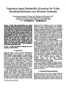
The core of the algorithm is as follows. If a node asks for more bandwidth, it will generate a query to all the nodes. Each node will send back some bandwidth according to availability or a well-defined traffic plan. The p2p paradigm is then applied both to the communication phase (i.e., no central authority mediates the interaction between two sensors) and to the bandwidth ownership relation (i.e., a centralized controller or marshaller owns the bandwidth). Let us analyze, in a more detailed fashion, the evolution of the virtual organization. As depicted in Figure 4, the overlaid network organization evolves during the algorithm lifetime; the very first snapshot, depicted in (a), shows that the virtual network acts on a client-server basis (where the BMP acts as a server). Later, as shown in (b), the bandwidth becomes distributed among quite a few sensors in the network. The BMP still plays a role, because a relevant amount of resource is under its supervision. In fact, the p2p organization is strictly related to the bandwidth ownership. Both in (a) and (b) there is a server-like entity that “owns” the resource (after the election): the key difference between (a) and (b) is that (a) represents a fully centralized approach, while (b) represents a hybrid scenario or a mediated p2p-network, where there are both centralized and distributed devices. The BMP delivers bandwidth, but normal sensors could directly manage a fraction of bandwidth. Finally, in (c) all the bandwidth has been distributed among all the requestors: each node now can act as a client (consuming bandwidth and asking for more) and server (delivering bandwidth). In this case, the organization is without any unique central point and

each sensor should be intended as “bandwidth peer”. In the figure, darker shadowing means more centralization. BMP

BMP

(a) client-server phase

(b) hybrid phase BMP

(c) pure p2p Figure 4. Different snapshots of the overall overlaid network.

The network kick-start phase is introduced to establish who is the very first owner of the bandwidth resource when the algorithm starts. Bandwidth policies are not strictly related with the proposed algorithm: actually, this algorithm introduces only a suitable method to exchange and distribute bandwidth on demand. Some constraints are needed to avoid starvation and uncontrolled bandwidth usage: policies’ exploitation needs a proper sub-layer in the layered architecture or a module inside the middleware layer.

b.

State Variables and Bandwidth Distribution

Before starting with a detailed explanation of the communication procedures, we must introduce the variables used to keep track of the bandwidth within the network and to define a state for each node.

The quantities introduced in (1) to (3) below allow defining the bandwidth available and actually used by every single node: they are the algorithm’s state variables.

Bi: the bandwidth available to the i-th node

(1)

Ui: the bandwidth used by the i-th node

(2)

Ri = Bi - Ui: the residual bandwidth of the i-th node

(3)

Each node updates its own state variables. The update is performed by the middleware, based on bandwidth requests both from the application layer and from other peers. The state variables are updated locally according to released, used, and received bandwidth. For instance, during a sensor’s lifetime, residual bandwidth could increase or decrease, depending upon applications running (e.g., the activation/deactivation of a video streaming function) or in response to bandwidth requests.

Let us analyze the algorithm’s evolution; there are three different basic events:

I)

A release-request is performed by processes running inside a node.

II)

A request arrives from a remote node.

III)

An answer is sent and received by a remote requestor.

Before analyzing the procedure, we will introduce the follow quantity.

RQi : an internal bandwidth update. This quantity carries the bandwidth requests/releases from

application processes.

Let us start by investigating when an internal release/request is performed. There are two different cases:

< 0 (bandwidth release) RQi =  > 0 (bandwidth request)

(4)

When RQi < 0 a process within a node performs a bandwidth release. The procedure is handled locally, without any external signaling flows: therefore, it will reflect only in a updating of the state variables stored in the middleware layer. The update is performed according to the following set of equations:

Binew ← Biold Uinew ←U iold + RQi

(5)

Rinew ← Binew −U inew = −U old − RQi = Riold − RQi = Bold i i

Conversely, when RQi > 0 , a process is requesting for more bandwidth. This will trigger two different temporal evolutions: if there is sufficient “internal” bandwidth, the action remains local at the node, but if the request is not fully satisfied, a bandwidth request is propagated to the network. At this stage there will be a “pending” bandwidth request waiting for a network response or another internal update. The pending status is recognizable by analyzing the sign of the residual bandwidth. If the residual bandwidth of a node is negative, the node is in a “bandwidth deficit” and is waiting for remote nodes’ responses to regain the positive sign and fully satisfy all the internal pending requests. Then,

← Bold Bnew i i

{

U new ← min U old + RQi , Bnew i i i

}

Rnew ← Rold − RQi = Bold −U old − RQi i i i i

(6)

If Rnew < 0 , there is a pending request: RQi is not fully satisfied. The amount of bandwidth still needed i is then

RQi ← Rnew i

(7)

The process is then iterated, assuming the previous quantity as a new bandwidth request. This will also trigger the signaling phase, asking other nodes for bandwidth.

Let us now analyze the evolution when an external request arrives, issued by a generic peer j. The algorithm will work at the maximum efficiency if each peer asks only for an amount of bandwidth really needed. Each peer, by using a “hot potato” approach, sends all its unused bandwidth back to the original requestor. Each peer will update its own state as follows:

for each responding peer

Bnew ← Bold − Rold i i i U new ←U old i i

(8)

Rnew ←0 i

The last action to be analyzed occurs when answers to a previously issued request arrive at node i. Let

RPi = ∑ Rrcvd j j≠i

where Rrcvd is the amount of bandwidth received from the j-th peer. j

(9)

The available bandwidth is then updated according to:

← Bold + RPi Bnew i i

(10)

and the used bandwidth becomes

← U old , if Rold ≥0 U new i i i

← U old − Rold , U new i i i if Rold < 0∧ Rold < RPi i i ← Bnew , U new i i < 0∧ Rold > RPi if Rold i i

(11)

Last, the residual bandwidth is updated according to the amounts received. Equations (12) and (13) below depict the residual bandwidth update and the amount of pending request, respectively.

← Bnew −U new ; Rnew i i i

(12)

>0)∨(Rold