A Perceptual Framework for Contrast Processing of High Dynamic ...

A Perceptual Framework for Contrast Processing of High Dynamic Range Images Rafał Mantiuk, Karol Myszkowski, and Hans-Peter Seidel MPI Informatik

Abstract Image processing often involves an image transformation into a domain that is better correlated with visual perception, such as the wavelet domain, image pyramids, multi-scale contrast representations, contrast in retinex algorithms, and chroma, lightness and colorfulness predictors in color appearance models. Many of these transformations are not ideally suited for image processing that significantly modifies an image. For example, the modification of a single band in a multi-scale model leads to an unrealistic image with severe halo artifacts. Inspired by gradient domain methods we derive a framework that imposes constraints on the entire set of contrasts in an image for a full range of spatial frequencies. This way, even severe image modifications do not reverse the polarity of contrast. The strengths of the framework are demonstrated by aggressive contrast enhancement and a visually appealing tone mapping which does not introduce artifacts. Additionally, we perceptually linearize contrast magnitudes using a custom transducer function. The transducer function has been derived especially for the purpose of HDR images, based on the contrast discrimination measurements for high contrast stimuli. CR Categories: I.3.3 [Computer Graphics]: Picture/Image Generation—Display algorithms; I.4.2 [Image Processing and Computer Vision]: Enhancement—Greyscale manipulation, sharpening and deblurring Keywords: visual perception, high dynamic range, contrast processing, tone mapping, contrast masking, contrast discrimination, transducer

1

Introduction and Previous Work

An image stored as a matrix of pixel values is the most common representation for image processing, but unfortunately it does not reflect the way we perceive images. This is why most image compression algorithms apply a transformation, such as the Discrete Cosine Transform or the Discrete Wavelet Transform before storing images, so that the visually important information is separated from visually unimportant noise. Besides image and video compression, there are many fields that benefit from a representation of images that is correlated with visual perception, such as tone mapping, visual difference prediction, color appearance modeling, or seamless image editing. The goal of such “perceptual” representations is to linearize values that encode images so that the magnitude of those values correspond to the visibility of features in an image. For example, large magnitudes of low and medium frequency coefficients c

ACM, 2006. This is the author’s version of the work. It is posted here by permission of ACM for your personal use. Not for redistribution.

of the Fourier Transform correspond to the fact that the visual system is the most sensitive for those frequencies. In this work we derive a framework for image processing in a perceptual domain of image contrast. We base our work on the gradient domain methods, which we generalize and extend to account for perceptual issues, such as the sensitivity for superthreshold contrast in HDR images. The research on perceptual representation of images has involved many areas of science. We briefly list some of these areas, pointing to the relevant works and describing major issues of these approaches. Image Transformations. A need for better image representation, which would partly reflect the processing of the Human Visual System (HVS), has been noticed in image processing for a long time. However, practical issues such as whether a transformation is invertible and computational costs, were often of more concern than an accurate modeling of the HVS. This resulted in numerous image transformations based in mathematics and signal processing, such as the Fourier transform, pyramids (Gaussian, Laplacian) or wavelets, which are now considered as standard tools of image processing. Color Appearance Models. Color appearance models, such CIECAM [CIE 2002] or iCAM [Fairchild and Johnson 2004], convert physical color values to a space of perceptual correlates, such as lightness, chroma and colorfulness. Such correlates are useful for the prediction of color appearance under different visual conditions, for finding visible differences in images and for tone mapping. The drawback of those models is that they do not account for aspects of spatial vision such as contrast sensitivity or contrast masking. Multi-scale Models of Human Vision. Spatial issues are better modelled with multi-scale models, such as those described in [Watson 1987; Simoncelli and Adelson 1989; ?; Winkler 2005], which separate an image into several band-pass channels. Such channels correspond to the visual pathways that are believed to exist in the HVS. Such models have been successfully applied for the prediction of visible differences in images [Daly 1993] and the simulation of color vision under different luminance adaptation conditions [Pattanaik et al. 1998]. However, they also pose many problems when images are modified in such multi-scale representations. If an image is modified in one of such band-pass limited channels while the other channels remain unchanged, the image resulting from the inverse transformation often contains severe halo artifacts. Retinex. A different set of problems has been addressed by the Retinex theory of color vision, introduced by Land [1964]. The original goal of Retinex was to model the ability of the HVS to extract reliable information from the world we perceive despite changes in illumination, which is referred as a color constancy. The latter work on the Retinex algorithm formalized the theory mathematically and showed that the problem is equivalent to solving a Poisson equation [Horn 1974; Hurlbert 1986]. Interestingly, most of the gradient methods also involve a solution of a Poisson equation although their goal is different. Gradient Methods. Operations on image gradients have recently attracted much attention in the fields of tone mapping [Fattal et al. 2002], image editing [Perez et al. 2003; Agarwala et al. 2004], im-

Forward Model Input Image

Transformation to Contrast

Contrast G

Transducer Function

Processing of Contrast

Inverse Model Output Image

Transformation to Luminance

Contrast G’

Response R

Inverse Transducer Function

Modified Response R’

Figure 1: Data flow in the proposed framework of the perceptual contrast processing.

age matting [Sun et al. 2004], image stitching [Levin et al. 2004], and color-to-gray mapping [Gooch et al. 2005]. The gradient methods can produce excellent results in areas where other methods usually result in severe artifacts. For instance, tone mapping and contrast enhancement performed in the gradient domain gives almost no halo artifacts while such artifacts are usually inevitable in the case of the multi-scale methods [Fattal et al. 2002]. The gradients methods can also seamlessly blend stitched images while other methods often result in visible discontinuities [Levin et al. 2004]. Even some advanced painting tools of Adobe Photoshop are based on the gradient methods [Georgiev 2005]. However, all these works focus mainly on image processing aspects without considering perceptual issues. In this work we generalize the gradient domain methods and incorporate perceptual issues by deriving a framework for processing images in perceptually linearized visual response space. Unlike the gradient or multi-scale methods, we impose constraints on the entire set of contrasts in an image for a full range of spatial frequencies. This way, even a severe image modification does not lead to reversing a polarity of contrast. This paper is an extended revision of a previous publication [Mantiuk et al. 2005]. The overview of our framework is shown in Figure 1. Pixel luminance values of an image are first transformed to physical contrast values, which are then transduced to response values of the HVS. The resulting image is then modified by altering the response values, which are closely related to a subjective impression of contrast. The modified response values can later be converted back to luminance values using an inverse transformation. As an application of our framework we demonstrate two tone mapping methods which can effectively compress dynamic range without losing lowcontrast information. We show that a complex contrast compression operation, which preserves textures of small contrast, is reduced to a linear scaling in our visual response space. In Section 2 we review less well known psychophysical data that was measured for high-contrast stimuli. Based on this data we derive a model of suprathreshold contrast discrimination for high contrast images. In Section 3 we introduce the components of our framework, in particular a multi-scale representation of low-pass contrast and a transducer function designed for HDR data. As an application of our framework, we propose two tone mapping methods in Sections 4 and 5, and a saliency preserving color to gray mapping in Section 6. Details on how the framework can be implemented efficiently are given in Section 7. We discuss strengths and weaknesses of the proposed framework in Section 9. Finally, we conclude and suggest future directions in Section 10.

W – contrast expressed as a Weber fraction (see Table 2) G – contrast expressed as a logarithmic ratio (see Table 2) ∆W (W ), ∆G(G) – function of threshold contrast discrimination for contrast W and G respectively ∆Gsimpl (G) – simplified function of threshold contrast discrimination for contrast G Gki, j – contrast between pixels i and j at the k’th level of a Gaussian pyramid (see Equation 6) Gˆ ki, j – modified contrast values, corresponding to Gki, j . Such contrast values usually do not form a valid image and only control an optimization procedure Lik – luminance of the pixel i at the k’th level of a Gaussian pyramid xik – log10 of luminance Lik Φi – set of neighbors of the pixel i T (G), T −1 (G) – transducer and inverse transducer functions R – response of the HVS scaled in JND units Rˆ – modified response R Table 1: Used symbols and notation.

2

Background

In the following two sections we review some fundamentals of the perception of contrast and summarize the results of a study on the HVS performance in contrast discrimination for HDR images. We use this contrast discrimination characteristic to derive our contrast processing framework.

2.1

Contrast

The human eye shows outstanding performance when comparing two light patches, yet it almost fails when assessing the absolute level of light. This observation can be confirmed in a ganzfeld, an experimental setup where the entire visual field is uniform. In fact, it is possible to show that the visual system cannot discern mean level variations unless they fluctuate in time or with spatial signals via eye movements, thus having a higher temporal frequency component. The Retinex theory postulated that low sensitivity to absolute luminance can be easily explained by the adaptation of the HVS to the real world conditions. Because the HVS is mostly sensitive to relative luminance ratios (contrast) rather than absolute luminance, the effect of huge light changes over the day is reduced and therefore we perceive the world in a similar way regardless of the light conditions. This and other sources of evidence strongly suggest that the perception of contrast (difference between two light stimuli) is the fundamental ability of the HVS. Many years of research on contrast have resulted in several definitions of contrast, some of them listed in Table 2. The variety of contrast definitions comes from the different stimuli they measure. For example, the Michelson contrast [Michelson 1927] is commonly used to describe a sinusoidal stimulus, while the Weber fraction is often used to measure a step increment or decrement stimulus. In the next section we show that certain contrast definitions are more suitable for describing the performance of the HVS than others.

0.1 Lmax

Simple Contrast Cs = LLmax min

Increments Decrements

∆L

Weber Fraction W = L∆L min

Lmin

Decrement

Lmax

∆L

Logarithmic Ratio G = log10 ( LLmax ) min

∆M

Increment

0.01

Lmin Lmax

Michelson Contrast |L −Lmin | M = Lmax max +Lmin

Lmean

Signal to Noise Ratio SNR = 20 · log10 ( LLmax ) min

0.001 1e−04

0.001

0.01

M

0.1

1

10

Lmin

Table 2: Definitions of contrast and the stimuli they measure. Contrast Discrimination Threshold ∆G(G) Contrast Detection Threshold G

Contrast Detection

Contrast Discrimination

Figure 2: The luminance profile of the stimuli used for contrast detection and contrast discrimination measurements. The test (red) and the standard (green) stimulus are displayed one after another. The threshold is the smallest visible contrast (detection) or a difference of contrast (discrimination).

2.2

Contrast Discrimination

Contrast detection and contrast discrimination are two of the most thoroughly studied perceptual characteristics of the eye [Barten 1999]. The contrast detection threshold is the smallest visible contrast of a stimulus presented on a uniform field, for example a Gabor patch on a uniform adaptation field. The contrast discrimination threshold is the smallest visible difference between two nearly identical signals, for example two sinusoidal patterns that differ only in their amplitudes. Detection can be considered as a special case of discrimination when the masking signal has zero amplitude. A difference between detection and discrimination tasks is illustrated in Figure 2. A stimulus can be considered suprathreshold when its contrast is significantly above the detection threshold. When the contrast is lower or very close to the detection threshold, a stimulus is considered subthreshold or threshold. Contrast discrimination is associated with the suprathreshold characteristics of the HVS and in particular with contrast masking. Contrast detection, on the other hand, describes the performance of the HVS for subthreshold and threshold stimulus, which can be modelled by the Contrast Sensitivity Function (CSF), the threshold versus intensity function (t.v.i.), or Weber’s law for luminance thresholds. The characteristic of contrast detection for a range of luminance adaptation levels is sometimes described as luminance masking. A good introduction to the above mentioned terminology can be found in [Wandell 1995, Chapter 7]. Since suprathreshold contrast plays a dominant role in the perception of HDR images, we will consider contrast discrimination data (suprathreshold) in detail and simplify the character of con-

Figure 3: Contrast discrimination thresholds plotted using the Michelson contrast, M. The Michelson contrast does not give a good prediction of the discrimination performance, especially for high contrast. trast detection (threshold). Although discrimination thresholds of the HVS have been thoroughly studied in psychophysics for years, most of the measurements consider only small contrast levels up to M = 50%. Such limited contrast makes the usefulness of the data especially questionable in the case of HDR images, for which the contrast can easily exceed 50%. The problem of insufficient scale of contrast in psychophysical experiments was addressed by Whittle [1986]. By measuring detection thresholds for the full range of visible contrast, Whittle showed that the discrimination data plotted with the Michelson contrast does not follow increasing slope, as reported in other studies (refer to Figure 3). He also argued that the Michelson contrast does not describe the data well. Figure 3 shows that the data is very scattered and the character of the threshold contrast is not clear, especially for large contrast values. However, when the same data is plotted as Weber’s fraction W = ∆L/Lmin , the discrimination thresholds for all but the smallest contrast values follow the same line on a log-log plot, which resembles Weber’s law, but for suprathreshold contrast: ∆W /W = c (see Figure 4). The sensitivity1 to contrast improves for low contrast just above the detection threshold and then deteriorates as the contrast reaches the threshold (W ≈ 0.025). Whittle calls this effect “crispening” while contrast discrimination studies usually describe it as a facilitation or “dipper” effect. Interestingly, typical models of contrast discrimination, such as Barten’s model [Barten 1999, Chapter 7], closely follow Whittle’s data for low contrast2 , but wrongly predict discrimination thresholds for high contrast (see the green solid line in Figure 4). The wrong prediction is a result of missing measurements for high contrast. Obviously, such models are not adequate for high contrast data, such as HDR images. To construct a model for contrast discrimination, which would be suitable for High Dynamic Range images, we fit a continuous function to Whittle’s original data [1986, Figure 2]: ∆W (W ) = 0.0928 ·W 1.08 + 0.0046 ·W −0.183

(1)

The chi-square test proves that the function approximates the data c

ACM, 2006. This is the author’s version of the work. It is posted here by permission of ACM for your personal use. Not for redistribution. 1

Sensitivity is defined as an inverse of the detection or discrimination threshold. 2 The parameters for Barten’s model have been chosen to fit the measurements by Foley and Legge [1981]. The detection threshold mt has been chosen so that it compensates for differences between the stimuli used for Whittle’s and Legge & Foley’s measurements.

1

100

∆W

10

Lmax

∆G(G)

∆W

Model fit to the data

W

0.1

Lmin

Barten’s Model

1

∆Gsimpl (G)

∆G

Luminance

1000

0.01 0.1 Increments Decrements

0.01 0.001 0.001

0.01

0.1

1 W

10

100

0.001

Figure 4: Contrast discrimination thresholds plotted as a function of contrast W . Data points – Whittle’s measurements; red solid line – a function fit to Whittle’s data; green solid line – Barten’s model fit to the measurements by Foley and Legge [1981] (k = 3, mt = 0.02); inset – the stimulus used to measure increments for Whittle’s data. (Q = 0.56) assuming a relative error ∆W /W ± 8%. The shape of the fitted function is shown as a red solid line in Figure 4. In Section 3.2 we use the above function rather than Whittle’s original model ∆W /W = c to properly predict discrimination thresholds for low contrast values. It is sometimes desirable to operate on contrast measure G rather than Weber fraction W (for contrast definitions refer to Table 2). In Section 3.1 we show that the proposed framework operates on contrast G since such contrast can be represented as a difference in logarithmic domain, which let us formulate a linear problem. Knowing that the relation between W and G is: G = log10 (W + 1)

(2)

and the relation between ∆W and ∆G is:  ∆W +1 , W +1 (3) we plot Whittle’s measurement points for contrast G in Figure 5. We can now fit the model from Equation 1 to the new data, to get a function of contrast discrimination for contrast G: ∆G ≈ log10 (W + ∆W + 1) − log10 (W + 1) = log10



∆G(G) = 0.0405 · G0.6628 + 0.00042435 · G−0.38072

(4)

The chi-square test for the fitted function gave Q = 0.86 assuming a relative error on ∆G/G ± 7%. If we do not need to model the facilitation effect or the loss of sensitivity for low contrast, we can approximate the data with a simpler function, which is both reversible and integrable, but does not consider data for G < 0.03: ∆Gsimpl (G) = 0.038737 · G0.537756

0.001

1000

(5)

The chi-square test for the fitted function gave Q = 0.88 assuming a relative error ∆G/G ± 3%. Both fitted functions are shown in Figure 5. Before we utilize the above discrimination functions, we have to consider whether it can be generalized for different stimuli and spatial frequencies. In a later study Kingdom and Whittle [1996] showed that the character of the suprathreshold discrimination is similar for both a square-wave and sine-wave patterns of different spatial frequencies. This is consistent with other studies that show

0.01

G

0.1

1

10

Figure 5: Contrast discrimination thresholds plotted as a function of the contrast G. The solid line – a full contrast discrimination model (Equation 4); the dashed line – a simplified contrast discrimination model (Equation 5). little variations of suprathreshold contrast across spatial frequencies [Georgeson and Sullivan 1975; Barten 1999]. Those variations can be eliminated if a contrast detection function is normalized by the contrast detection threshold for a particular spatial frequency [Legge 1979].

3

Framework for Perceptual Contrast Processing

In the next two sections we introduce a framework for image processing in a visual response space. Section 3.1 proposes a method for transforming complex images from luminance to physical contrast domain (blocks Transform to Contrast and Transform to Luminance in Figure 1). Section 3.2 explains how physical contrast can be converted into a response of the HVS, which is a perceptually linearized measure of contrast (blocks Transducer Function and Inverse Transducer Function in Figure 1).

3.1

Contrast in Complex Images

Before we introduce contrast in complex images, let us consider the performance of the eye during discrimination of spatially distant patches. We can easily observe that contrast can be assessed only locally for a particular spatial frequency. We can, for example, easily see the difference between fine details if they are close to each other, but we have difficulty distinguishing the brighter detail from the darker if they are distant in our field of view. On the other hand, we can easily compare distant light patches if they are large enough. This observation can be explained by the structure of the retina, in which the foveal region responsible for the vision of fine details spans only about 1.7 visual degrees, while the parafoveal vision can span over 160 visual degrees, but has almost no ability to process high frequency information [Wandell 1995]. When seeing fine details in an image, we fixate on a particular part of that image and employ the foveal vision. But at the same time the areas further apart from the fixation point can only be seen by the parafoveal vision, which can not discern high frequency patterns. The contrast discrimination for spatial patterns with increasing separation follows Weber’s law when the eye is fixed to one of the patterns and this is the result of the increasing eccentricity of the other pattern [Wilson 1980]. Therefore, due to the structure of the retina, the

ˆ This can be achieved by the but not necessarily exactly equal to G. minimization of the distance between a set of contrast values Gˆ that specifies the desired contrast, and G, which is the contrast of the actual image. This can be formally written as the minimization of the objective function:

1

G 12, 8 x1 x2 x3 x4 x5 x6 x7 x8 x9 x10 x11 x12 x13 x14 x15 x16 x17 x18 x19 x20 x21 x22 x23 x24 x25

1 )= f (x11 , x21 , . . . , xN

Figure 6: Contrast values for the pixel x12 (blue) at a single level of the Gaussian pyramid. The neighboring pixels x j are marked with green color. Note that the contrast value G12,7 (upper index k = 1 omitted for clarity) will not be computed, since G7,12 already contains the same difference. Contrast values G12,8 and G12,18 encode contrast for diagonal orientations. Unlike wavelets, contrast values, Gki, j can represent both −45◦ and 45◦ orientation. distance at which we can correctly assess contrast is small for high frequency signals, but grows for low frequency signals. While several contrast definitions have been proposed in the literature (refer to Table 2), they are usually applicable only to a simple stimulus and do not specify how to measure contrast in complex scenes. This issue was addressed by Peli [1990] who noticed that the processing of images is neither periodic nor local and therefore the representation of contrast in images should be quasi-local as well. Drawing analogy from the center-surround structures in the retina, he proposed to measure contrast in complex images as a difference between selected levels of a Gaussian pyramid. However, the resulting difference of Gaussians leads to a band-pass limited measure of contrast, which tends to introduce halo artifacts at sharp edges when it is modified. To avoid this problem, we introduce a low-pass measure of contrast. We use a logarithmic ratio G as the measure of contrast between two pixels, which is convenient in computations since it can be replaced with the difference of logarithms. Therefore, our low-pass contrast is defined as a difference between a pixel and one of its neighbors at a particular level, k, of a Gaussian pyramid, which can be written as: Gki, j = log10 (Lik /Lkj ) = xik − xkj

(6)

where Lik and Lkj are luminance values for neighboring pixels i and j. For a single pixel i there are two or more contrast measures Gki, j , depending on how many neighbouring pixels j are considered (see Figure 6). Note that both L and x cover a larger and larger area of an image when moving to the coarser levels of the pyramid. This way our contrast definition takes into account the quasi-local perception of contrast, in which fine details are seen only locally, while variations in low frequencies can be assessed for the entire image. The choice of how many neighboring pixels, x j , should be taken into account for each pixel, xi , usually depends on the application and type of images. For tone mapping operations on complex images, we found that two nearest neighbors are sufficient. For other applications, such as a color-to-gray mapping, and for images that contain flat areas (for example vector maps), we consider 20–30 neighboring pixels. Equation 6 can be used to transform luminance to contrast. Now we would like to perform the inverse operation that restores an image ˆ The problem is that there is from the modified contrast values G. probably no image that would match such contrast values. Therefore, we look instead for an image whose contrast values are close

K

N

∑∑ ∑

k=1 i=1 j∈Φi

pki, j (Gki, j − Gˆ ki, j )2

(7)

with regard to the pixel values xi1 on the finest level of the pyramid. Φi is a set of the neighbors of the pixel i (e.g. set of green pixels in Figure 6), N is the total number of pixels and K is the number of levels in a Gaussian pyramid. We describe an efficient solution of the above minimization problem in Section 7. The coefficient pki, j in Equation 7 is a constant weighting factor, which can be used to control a mismatch between the desired contrast and the contrast resulting from the solution of the optimization problem. If the value of this coefficient is high, there is higher penalty for a mismatch between Gki, j and Gˆ ki, j . Although the choice of these coefficients may depend on the application, in most cases we want to penalize contrast mismatch relative to the contrast sensitivity of the HVS. A bigger mismatch should be allowed for the contrast magnitudes to which the eye is less sensitive. This way, the visibility of errors resulting from such a mismatch would be equal for all contrast values. We can achieve this by assuming that: pki, j

=



if Gˆ ki, j ≥ 0.001 otherwise,

∆G−1 (Gˆ ki, j ) ∆G−1 (0.001)

(8)

where ∆G−1 is an inverse of the contrast discrimination function from Equation 4 and the second condition avoids division by 0 for very low contrast. When testing the framework with different image processing operations, we noticed that the solution of the optimization problem may lead to reversing polarity of contrast values in an output image, which happens when Gki, j is of a different sign than Gˆ ki, j , and which leads to halo artifacts. This problem concerns all methods that involve a solution of the optimization problem similar to the one given in Equation 7 and is especially evident for the gradients domain method (based on Poisson solvers). The problem is illustrated in Figure 7. To simplify the notation, the upper index of a Gaussian pyramid level is assumed to be 1 and is omitted. A set of desired contrast values Gˆ quite often contains the values that cannot lead to any valid pixel values (7a). The solution of the optimization problem results in modified contrast values G that can be used to construct an image with pixel values x1 , x2 , x3 (7b). The problem is that this solution results in a reversed polarity of contrast (G3,1 in 7b), which leads to small magnitude, but noticeable, halo artifacts. More desirable would be solution (7c), which gives the same value of the objective function f and does not result in reverse contrast values. To increase probability that the optimization procedure results in solution (7c) rather than (7b), the objective function should be penalized for mismatches at low contrast. This can be combined together with penalizing mismatches according to the sensitivity of the HVS if we replace the contrast discrimination function ∆G in Equation 8 with the simplified model ∆Gsimpl from Equation 5: pki, j =

1 ∆Gsimpl (Gˆ ki, j )

(9)

The simplified model overestimates sensitivity for low contrast, which is desirable as it makes the value of pki, j large near zero contrast and thus prevents the reversal of contrast polarity.

Gˆ 2,1

Gˆ 3,1

160

Gˆ 3,2 G2,1 G3,1

b)

G3,2 x1

x3

x2 G2,1

G3,1

c)

x1

x2

R = T (G)

80

3

60

2

0

∆T = 1JND

1 0

0

2

4

6

∆G(Gthreshold ) G

Gthreshold

8 Contrast G

10

12

14

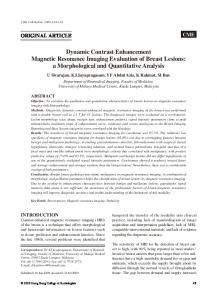
Figure 8: Transducer function derived from the contrast discrimination data [Whittle 1986]. The transducer function can predict the response of the HVS for the full range of contrast. The inset depicts how the transducer function is constructed from the contrast discrimination thresholds ∆G(G).

Transducer Function

A transducer function predicts the hypothetical response of the HVS for a given physical contrast. As can be seen in Figure 1, our framework assumes that the image processing is done on the response rather than on the physical contrast. This is because the response closely corresponds to the subjective impression of contrast and therefore any processing operations can assume the same visual importance of the response regardless of its actual value. In this section we would like to derive a transducer function that would predict the response of the HVS for the full range of contrast, which is essential for HDR images. Following [Wilson 1980] we derive the transducer function T (G) := R based on the assumption that the value of the response R should change by one unit for each Just Noticeable Difference (JND) both for threshold and suprathreshold stimuli. However, to simplify the case of threshold stimuli, we assume that:

or

R

100

20

Figure 7: For a set of desired contrast values Gˆ i, j that cannot represent a valid image (a), the optimization procedure may find a solution which contains reversed contrast values (G3,1 in b). An alternative solution without such reversed contrast values gives images without halo artifacts (c).

3.2

120

40 G3,2

x3

R = T (G)

140 Response R [JND]

a)

180

T (0) = 0 and T (Gthreshold ) = 1

(10)

T −1 (0) = 0 and T −1 (1) = Gthreshold

(11)

for the inverse response function T −1 (R) = G and for the boundary condition from Equation 11. G is a non-negative logarithmic ratio (refer to Table 2) and R is the response of the HVS. Since the function T −1 is strictly monotonic, finding the function T is straightforward. We numerically solve Equation 13 to find the transducer function T (G) = R shown in Figure 8. For many applications an analytical model of a transducer function is more useful than a lookup table given by the numerical solution of Equation 13. Although the curve shown in Figure 8 closely resembles a logarithmic or exponential function, neither of these two families of functions give an exact fit to the data. However, if an accurate model is not necessary, the transducer can be approximated with the function: T (G) = 54.09288 · G0.41850

The average and maximum error of this approximation is respectively R ± 1.9 and R ± 6. Equation 14 leads directly to an inverse transducer function: T −1 (R) = 7.2232 · 10−5 · R2.3895 .

T −1 (R)

for the inverse transducer function := G. The detection threshold, Gthreshold , is approximated with 1% contrast (Gthreshold = log10 (0.01 + 1) ≈ 0.0043214), commonly used for digital images [Wyszecki and Stiles 2000, Section 7.10.1]. This simplification assumes that the detection threshold is the same for all spatial frequencies and all luminance adaptation conditions. For a suprathreshold stimulus we approximate the response function T by its first derivative: ∆T ≈

dT (G) ∆G(G) = 1 dG

(12)

where ∆G(G) is the discrimination threshold given by Equation 4. The above equation states that a unit increase of response R (right hand side of the equation) should correspond to the increase of G equal to the discrimination threshold ∆G for the contrast G (left side of the equation). The construction of the function R = T (G) is illustrated in the inset of Figure 8. Although the above equation can be solved by integrating its differential part, it is more convenient to solve numerically the equivalent differential equation: dT −1 (R) = ∆G(T −1 (R)) dR

(13)

(14)

(15)

The transducer function derived in this section has a similar derivation and purpose as the Standard Grayscale Function from the DICOM standard [DICOM 2001] or the capacity function in [Ashikhmin 2002]. The major difference is that the transducer function operates in the contrast domain rather than in the luminance domain. It is also different from other transducer functions proposed in the literature (e.g. [Wilson 1980; Watson and Solomon 1997]) since it is based on the discrimination data for high contrast and operates on contrast measure G. This makes the proposed formulation of the transducer function especially suitable to HDR data. The derived function also simplifies the case of the threshold stimuli and assumes a single detection threshold Gthreshold . Such a simplification is acceptable, since our framework focuses on suprathreshold rather than threshold stimuli.

4

Application: Contrast Mapping

In previous sections we introduce our framework for converting images to perceptually linearized contrast response and then restoring

Figure 9: The results of the contrast mapping algorithm. The images from left to right were processed with the compression factor l = 0.1, 0.4, 0.7, 1.0. After the processing images were rescaled in the log 10 domain to use the entire available dynamic range. Memorial Church image courtesy of Paul Debevec. images from the modified response. In this section we show that one potential application of this framework is to compress the dynamic range of HDR images to fit into the contrast reproduction capabilities of display devices. We call this method contrast mapping instead of tone mapping because it operates on contrast response rather than luminance. Tone mapping algorithms try to overcome either the problem of the insufficient dynamic range of a display device (e.g. [Tumblin and Turk 1999; Reinhard et al. 2002; Durand and Dorsey 2002; Fattal et al. 2002]) or the proper reproduction of real-word luminance on a display (e.g. [Pattanaik et al. 1998; Ashikhmin 2002]). Our method does not address the second issue of trying to make images look realistic and natural. Instead we try to fit to the dynamic range of the display so that no information is lost due to saturation of luminance values and at the same time, small contrast details, such as textures, are preserved. Within our framework such nontrivial contrast compression operation is reduced to a linear scaling in the visual response space. Since the response Rki, j is perceptually linearized, contrast reduction can be achieved by multiplying the response values by a constant l: Rˆ ki, j = Rki, j · l

(16)

where l is between 0 and 1. This corresponds to lowering the maximum contrast that can be achieved by the destination display. Since the contrast response R is perceptually linearized, scaling effectively enhances low physical contrast W , for which we are the most sensitive, and compresses large contrast magnitudes, for which the sensitivity is much lower. The result of such contrast compression for the Memorial Church image is shown in Figure 9. In many aspects the contrast compression scheme resembles the gradient domain method proposed by Fattal et al. [2002]. However, unlike the gradient method, which proposes somewhat ad-hoc choice of the compression function, our method is entirely based on the perceptual characteristic of the eye. Additionally, our method can avoid low frequency artifacts as discussed in Section 9. We tested our contrast mapping method on an extensive set of HDR images. The only visible problem was the magnification of the camera noise on several HDR photographs. Those pictures were most likely taken in low light conditions and therefore their noise level

was higher than in the case of most HDR photographs. Our tone mapping method is likely to magnify camera noise if its amplitude exceeds the threshold contrast Wthreshold of the HVS. Therefore, to obtain good results, the noise should be removed from images prior to the contrast mapping. In Figure 11 we compare the results of our method with other tone mapping algorithms. Our contrast mapping method produces very sharp images without introducing halo artifacts. Sharpening is especially pronounced when the generated images are compared to the result of linear scaling in the logarithmic domain (see Figure 12).

5

Application: Contrast Equalization

Histogram equalization is another common method to cope with extended dynamic range. Even if high contrast occupies only a small portion of an image, it is usually responsible for large dynamic range. The motivation for equalizing the histogram of contrast is to allocate dynamic range for each contrast level relative to the space it occupies in an image. To equalize a histogram of contrast responses, we first find the Cumulative Probability Distribution Function (CPDF) for all contrast response values in the image Rki, j [Gonzalez and Woods 2001, Section 3]. Then, we calculate the modified response values: Rˆ ki, j = sign(Rki, j ) ·CPDF(kRki k)

(17)

where sign() equals −1 or 1 depending on the sign of the argument and kRki k is a root-mean-square of the contrast response between a pixel and all its neighbors: s 2 kRki k = (18) ∑ Rki, j j∈Φi

The histogram equalization scheme produces very sharp and visually appealing images, which may however be less natural in appearance than the results of our previous method (see some examples in Figures 10, 11, and 12). Such a tone mapping method can be especially useful in those applications, where the visibility of small

Figure 10: Top left – the linear rescaling of luminance in the logarithmic domain; top right – contrast mapping; bottom left – contrast equalization; bottom right – the result of [Reinhard et al. 2002]. Image courtesy of Grzegorz Krawczyk. details is paramount. For example, it could be used to reveal barely visible details in forensic photographs or to improve the visibility of small objects in satellite images. The results of the contrast equalization algorithm may appear like the effect of a sharpening filter. Figure 13 shows that the result of the contrast equalization (b) results in an image of much better contrast than the original image (a) while preserving low frequency global contrast. Sharpening filters tend to enhance local contrast at the cost of global contrast, which results in images that have flat appearance (c,d). Sharpening filters also introduce ringing and halo artifacts, especially in the areas of high local contrast, such as the border of the window in Figure 13 (c,d). The results of the contrast equalization algorithm are free of these artifacts.

6

Application: Color to Gray

Color images can often lose important information when printed in grayscale. Take for example Figure 15, where the sun disappears from the sky when only luminance is computed from the color image. The problem of proper mapping from color to grayscale has been addressed in numerous works, recently in [Gooch et al. 2005; Rasche et al. 2005]. We implemented the approach of Gooch et al. [2005] since their solution can be easily formulated within our framework. Their algorithm separately computes luminance and chrominance differences in a perceptually uniform CIE L ∗ a∗ b∗ color space for low-dynamic range. Such differences correspond to contrast values, G1i, j , in our framework (the finest level of a Gaussian pyramid). To avoid artifacts in flat areas (more on this in Section 9), their algorithm computes differences between all pixels in

the image, which is equivalent to considering for each pixel, x i , all remaining pixels in the image as neighbors, x j . Next, each luminance difference that is smaller than the corresponding chrominance difference is replaced with that chrominance difference. The algorithm additionally introduces parameters that control polarity of the chrominance difference, and the amount of chromatic variation applied to the luminance values. Finally, they formulate an optimization problem that is equivalent to Equation 7 restricted to the finest level of a pyramid (k = 1). The result of the optimization gives a gray-scale image that preserves color saliency. The authors show that their method produces results without artifacts for a broad range of images. The algorithm, while giving excellent results, is prohibitively computationally expensive and feasible only for very small images. This is because it computes differences (contrast values) between all pixels in an image, what gives a minimum complexity of O(N 2 ) regardless of the optimization method used. The number of considered differences can be limited, however at the cost of possible artifacts in isoluminant regions. Our framework involves a more efficient approach, in which the close neighborhood of a pixel is considered on fine levels of a Gaussian pyramid while far neighborhood is covered on coarser levels. This let us work with much bigger images and perform computations much faster. Following [Gooch et al. 2005] we transform input images into a CIE L∗ a∗ b∗ color space. Then, we transform each color channel into a pyramid of contrast values using Equation 6 (but xik denotes now the values in color channels). Next, we compute the color difference: q k∆Ci,k j k = (G(a∗ )ki, j )2 + (G(b∗ )ki, j )2 (19)

Figure 11: Comparison of the result produced by our contrast mapping (top left) and contrast equalization (top right) to those of Durand and Dorsey [2002] (bottom left) and Fattal et al. [2002] (bottom right). Tahoma image courtesy of Greg Ward.

Figure 12: The linear rescaling of luminance in the logarithmic domain (left) compared with two proposed contrast compression methods: contrast mapping (middle) and contrast equalization (right).

Figure 13: The contrast equalization algorithm compared with sharpening filters. (a) the original image; (b) the result of contrast equalization; (c) the result of a ’local adaptation’ sharpening; (d) the result of a sharpening filter. and selectively replace G(L∗ )ki, j with a signed k∆Ci,k j k, like in [Gooch et al. 2005]. We consider difference values for each level of a Gaussian pyramid and for 20–30 neighboring pixels. There is no need to apply the transducer function to the data. The reconstructed images can be seen in Figure 14 and 15. We achieve images of similar quality as [Gooch et al. 2005], but at a significantly lower computational cost.

7

Image Reconstruction from Contrast

In this section we give an efficient solution to the optimization problem stated in Section 3.1. By solving the optimization problem, we can reconstruct an output image from modified contrast values. The major computational burden of our method lies in minimizing the objective function given in Equation 7. The objective function reaches its minimum when all its derivatives ∂∂ xf equal 0: i

K N ∂f = ∑ ∑ ∑ 2pki, j (xik − xkj − Gˆ ki, j ) = 0 ∂ xi k=1 i=1 j∈Φi

(20)

for i = 1, . . . , N. The above set of equations can be rewritten using a matrix notation: A·X = B (21) where X is a column vector of x1 , . . . , xN , which holds pixel values of the resulting image, A is an N × N square matrix and B is an N-row vector. For a few mega-pixel images N can equal several million and therefore Equation 21 involves the solution of a huge set of linear equations. For a sparse matrix A a fast solution of such a problem can be found using multi-grid methods. However, since we consider contrast at all levels of a Gaussian pyramid, the matrix A in our case is not sparse. From the visualization of the matrix A (see Figure 16), we can conclude that the matrix has a regular

Figure 14: Examples of a saliency preserving color to gray mapping. Left – original image; center – luminance image; right – the result of the color to gray algorithm. Images courtesy of Jay Neitz(top) and Karl Rasche(bottom) structure, but certainly cannot be considered sparse. Such multiresolution problem seems to be well suited for the Fourier methods [Press et al. 2002, Chapter 19.4]. However, the problem cannot be solved using those methods either, since they require matrix coefficients to be of the same value while the constant factors pki, j introduce variations between matrix coefficients. We have found that the biconjugate gradient method [Press et al. 2002, Chapter 2.7] is appropriate for our problem and gives results in acceptable time. The biconjugate gradient method is considered to be slower than more advanced multi-grid methods, however we found that it converges equally fast for our problem. This is because the structure of the A matrix enforces that iterative improvements are performed for all spatial frequencies of an image, which is also the goal of multi-grid methods. The biconjugate gradient method is also often used as a part of a multi-grid algorithm. The biconjugate gradient method involves an iterative procedure, in which an image stored in the vector X is refined in each iteration. The attractiveness of this method is that it requires only an efficient computation of the product Ψ = A · X. For clarity consider only the nearest neighborhood of each pixel, although the algorithm can be easily generalized to a larger pixel neighborhood at moderate computational cost. The contrast is computed between a pixel and its four neighbors within the same level of a Gaussian pyramid. Let X k be a matrix holding pixel values of an image at the k-level of a Gaussian pyramid. Then, we can compute the product Ψ using the following recursive formula: Ψk (X k ) = X k × L + upsample[Ψk+1 (downsample[X k ])], (22) where X k is a solution at the k-th level of the pyramid, the operator × denotes convolution, L is the kernel   0 1 0 L =  1 −4 1  (23) 0 1 0

Figure 15: An example of a saliency preserving color to gray mapping. Left – original image; center – luminance image; right – the result of the color to gray algorithm. Image: Impressionist Sunrise by Claude Monet transferred from an original image. The goal is to preserve the same perceived hue and color saturation while altering luminance. Hue can be easily preserved if a color space that decorrelates chrominance from luminance is used (such as LHS or Yxy). Preserving the perceived color saturation is much more difficult since it is strongly and non-linearly correlated with luminance. Additionally, the perceived color saturation may change if luminance contrast is modified. A transfer of color saturation seems to be a difficult and still unsolved problem. Therefore, for the proposed tone mapping algorithms, we follow the method employed in most tone mapping algorithms, which involves rescaling red, green and blue color channels proportionally to the luminance and desaturating colors to compensate for higher local contrast. For each pixel, we compute:

Figure 16: Visualization of the matrix A, which is involved in the solution of the optimization problem for a 1-mega-pixel image. White color denotes zero coefficients, which increase in magnitude with darker colors. Gray corresponds to positive and green to negative coefficients. and upsample[] and downsample[] are image upsampling and downsampling operators. The recursion stops when one of the image dimensions is less than 3 pixels after several successive downsamplings. The right-hand term B can be computed using another recursive formula: Bk (Gˆ k ) = Gˆ k:,x × Dx + Gˆ k:,y × Dy + + upsample[Bk+1 (downsample[Gˆ k ])]

(24)

Gˆ k

where is the modified contrast at the k-th level of the pyramid, Gˆ k:,x and Gˆ k:,y are the subsets of contrast values Gˆ k for horizontal and vertical neighbors, and Dx, Dy are the convolution kernels:     1 (25) Dx = 1 −1 Dy = −1

For simplicity, we did not include the coefficients pki, j in the above equations. Note that if only the first level of the pyramid is considered, the problem is reduced to the solution of Poisson’s equation as in [Fattal et al. 2002]. To account for the boundary conditions, we can pad each edge of an image with a line or column that is a replica of the image edge.

8

Reconstruction of Color

Many applications, including the majority of tone mapping algorithms, focus on the processing of luminance while chrominance is

Cout =

X − lmin + s(Cin − Lin ) lmax − lmin

(26)

where Cin and Cout are the input and output pixel values for the red, green or blue color channel, Lin is the input luminance, and X is the result of the optimization (all values are in the logarithmic domain). The resulting values Cout are within the range from 0 to 1. The parameter s is responsible for the saturation of colors and is usually set between 0.4 and 0.6. If Pk is k-th percentile of X and d = max(P50 − P0.1 , P99.9 − P50 ), then lmin = P50 − d and lmax = P50 + d. This way, the average gray level is mapped to the gray level of the display (r = g = b = 0.5) and overall contrast is not lost due to a few very dark or bright pixels. Note that fine tuning of lmax and lmin values is equivalent to so called gammacorrection used as a last step of many tone mapping algorithms. This is because a power function in the linear domain corresponds to a multiplication in the logarithmic domain: log(xγ ) = γ · log(x). Equation 26 is similar to formulas proposed by Tumblin and Turk [1999] but it is given in the logarithmic domain and includes a linear scaling. The resulting color values, Cout , can be linearly mapped directly to the pixel values of a gamma corrected (perceptually linearized) display.

9

Discussion

The proposed framework is most suitable for those problems where the best solution is a compromise between conflicting goals. For example, in the case of contrast mapping (Section 4), we try to compress an overall contrast by suppressing low frequencies (low frequency contrast has large values and thus is heavily compressed), while preserving details. However, when enhancing details we also lessen compression of overall contrast since details can span a broad range of spatial frequencies (the lower levels of low-pass Gaussian pyramid) including low-frequencies, which are primarily responsible for an overall contrast. The strength of our method comes

Figure 17: When an original signal (upper left) is restored from attenuated gradients (upper right) by solving Poisson’s equation (or integration in 1-D), the flat parts of the restored signal are shifted relative to each other (lower left). However, if the minimization constraints are set for multiple levels of the pyramid as in our proposed method, the flat parts can be accurately restored although the sharp peaks are slightly blurred (lower right). from the fact that the objective function given in Equation 7 leads to a compromise between the conflicting goals of compressing lowfrequency large contrast and preserving small contrast of the details. The minimization problem introduced in Equation 7 seems similar to solving Poisson’s equation in order to reconstruct an image from gradients, as proposed by Fattal et al. [2002]. The difference is that our objective function takes into account a broader neighborhood of a pixel (summation over j) and puts additional optimization constraints on the contrast at coarser levels of the pyramid (summation over l), which improves a restoration of low frequency information. When an objective function is limited only to the finest level of the Gaussian pyramid (as it is done in Poisson’s equation), the low frequency content may be heavily distorted in the resulting image 3 . This is illustrated on the examples of a 1-D signal in Figure 17 and a tone-mapped image in Figure 18. In general, Poisson solvers may lead to the reduction (or even reversal) of global low-frequency contrast measured between disconnected image fragments. Other researchers have also noticed this problem. Gooch at al. [2005] experimented with Poisson solvers and found that they do not work well for “large disconnected isoluminant regions because they compute gradients over nearest neighbors, ignoring difference comparison over distances greater than one pixel”. They overcome this problem by including a larger number of neighbors for each pixel in the objective function. The importance of global contrast and the fact that considering only local contrast gives wrong results was also discussed in [Rasche et al. 2005, Figure 2]. Our framework can be considered as a generalization of the gradient domain methods based on Poisson solvers. We consider larger neighborhoods for local contrast and also several levels of a Gaussian pyramid for global contrast. Such an approach is both perceptually plausible and computationally much more efficient than solving the optimization problem for contrast values between all pixels in the image [Gooch et al. 2005]. The most computationally expensive part of the proposed framework is the contrast-to-luminance transformation. The solution of the minimization problem for 1–5 Mpixel images can take from several seconds up to half a minute to compute on a modern PC. This limits the application of the algorithm to off-line processing. c

ACM, 2006. This is the author’s version of the work. It is posted here by permission of ACM for your personal use. Not for redistribution. 3

Loss of low-frequency contrast is also visible in Figure 3 in the paper by Fattal et al. [2002], where low intensity levels of the left and middle peaks in the original image (a) are strongly magnified in the output image (f), so that they eventually become higher than the originally brightest image part on the right side.

Figure 18: The algorithm by Fattal et al. [2002] (top) renders windows panes of different brightness due to the local nature of the optimization procedure. The contrast compression on the multi-scale contrast pyramid used in our method can maintain proper global contrast proportions (bottom). Image courtesy of Greg Ward.

However, our solution is not much less efficient than multi-grid methods (for example [Fattal et al. 2002]) as discussed in Section 7.

10

Conclusions and Future Work

In this paper we have presented a framework for image processing operations that work in the visual response space. Our framework is in many aspects similar to the gradient methods based on solving Poisson’s equation, which prove to be very useful for image and video processing. Our solution can be regarded as a generalization of these methods which consider contrast on multiple spatial frequencies. We express a gradient-like representation of images using physical and perceptual terms, such as contrast and visual response. This gives perceptual basis for the gradient methods and offers several extensions from which these methods can benefit. For instance, unlike the solution of Poisson’s equation, our pyramidal contrast representation ensures proper reconstruction of low frequencies and does not reverse global brightness levels. We also introduce a transducer function that can give the response of the HVS for the full range of contrast amplitudes, which is especially desired in case of HDR images. Some applications can also make use of the contrast discrimination thresholds, which describe

suprathreshold performance of the eye from low to high contrast. As a proof of concept, we implemented two tone mapping algorithms and a saliency preserving color to gray mapping inside our framework. The tone mapping was shown to produce sharper images than the other contrast reduction methods. We believe that our framework can also find many applications in image and video processing. In the future, we would like to improve the performance of reconstructing the image from the contrast representation, which would make the framework suitable for real-time applications. We would also like to include color information using a representation similar to luminance contrast. The framework could be extended to handle animation and temporal contrast. Furthermore, the accuracy of our model can be improved for the threshold contrast if the Contrast Sensitivity Function were taken into account in the transducer function. A simple extension is required to adapt our framework to the task of predicting visible differences in HDR images: since the response in our framework is in fact scaled in JND units, the difference between response values of two images gives the map of visible differences. One possible application of such HDR visible difference predictor could be the control of global illumination computation by estimating visual masking [Ramasubramanian et al. 1999; Dumont et al. 2003]. Finally, we would like to experiment with performing common image processing operations in the visual response space.

11

Acknowledgments

We would like to thank Dani Lichinski for helpful discussion on his gradient domain method. We are also grateful for his patience in generating images using his tone mapping method. We also thank Kaleigh Smith for proofreading the manuscript.

References AGARWALA , A., D ONTCHEVA , M., AGRAWALA , M., D RUCKER , S., C OLBURN , A., C URLESS , B., S ALESIN , D., AND C OHEN , M. 2004. Interactive digital photomontage. ACM Transactions of Graphics. 23, 3, 294–302. A SHIKHMIN , M. 2002. A tone mapping algorithm for high contrast images. In Rendering Techniques 2002: 13th Eurographics Workshop on Rendering, 145–156. BARTEN , P. G. 1999. Contrast sensitivity of the human eye and its effects on image quality. SPIE – The International Society for Optical Engineering. ISBN 0-8194-3496-5. CIE. 2002. A Colour Appearance Model for Colour Management Systems: CIECAM02 (CIE 159:2004). DALY, S. 1993. The Visible Differences Predictor: An algorithm for the assessment of image fidelity. In Digital Image and Human Vision, Cambridge, MA: MIT Press, A. Watson, Ed., 179–206. DICOM. 2001. Part 14: Grayscale standard display function. In Digital Imaging and Communications in Medicine (DICOM). D UMONT, R., P ELLACINI , F., AND F ERWERDA , J. A. 2003. Perceptuallydriven decision theory for interactive realistic rendering. ACM Transactions on Graphics 22, 2 (Apr.), 152–181. D URAND , F., AND D ORSEY, J. 2002. Fast bilateral filtering for the display of high-dynamic-range images. ACM Transactions on on Graphics 21, 3, 257–266.

FAIRCHILD , M., AND J OHNSON , G. 2004. icam framework for image appearance differences and quality. Journal of Electronic Imaging 13, 1, 126–138. FATTAL , R., L ISCHINSKI , D., AND W ERMAN , M. 2002. Gradient domain high dynamic range compression. ACM Transactions on Graphics 21, 3, 249–256. F OLEY, J., AND L EGGE , G. 1981. Contrast detection and near-threshold discrimination in human vision. Vision Research 21, 1041–1053. G EORGESON , M., AND S ULLIVAN , G. 1975. Contrast constancy: Deblurring in human vision by spatial frequency channels. J.Physiol. 252, 627–656. G EORGIEV, T. 2005. Vision, healing brush, and fiber bundles. In IS&T/SPIE Conf. on Hum. Vis. and Electronic Imaging X, vol. 5666, 293–305. G ONZALEZ , R. C., AND W OODS , R. E. 2001. Digital Image Processing, 2nd Edition. G OOCH , A. A., O LSEN , S. C., T UMBLIN , J., AND G OOCH , B. 2005. Color2gray: Salience-preserving color removal. ACM Transactions on Graphics 24, 3. H ORN , B. 1974. Determining lightness from an image. Computer Graphics and Image Processing 3, 1, 277–299. H URLBERT, A. 1986. Formal connections between lightness algorithms. Journal of the Optical Society of America A 3, 10, 1684–1693. K INGDOM , F. A. A., AND W HITTLE , P. 1996. Contrast discrimination at high contrasts reveals the influence of local light adaptation on contrast processing. Vision Research 36, 6, 817–829. L AND , E. H. 1964. The retinex. American Scientist 52, 2, 247–264. L EGGE , G. 1979. Spatial frequency masking in human vision: binocular interactions. Journal of the Optical Society of America 69, 838–847. L EVIN , A., Z OMET, A., P ELEG , S., AND W EISS , Y. 2004. Seamless image stitching in the gradient domain. In Eighth European Conference on Computer Vision, vol. 4, 377–389. M ANTIUK , R., M YSZKOWSKI , K., AND S EIDEL , H.-P. 2005. A perceptual framework for contrast processing of high dynamic range images. In APGV ’05: Proceedings of the 2nd symposium on Appied perception in graphics and visualization, ACM Press, New York, NY, USA, 87–94. M ICHELSON , A. 1927. Studies in Optics. U. Chicago Press. PATTANAIK , S. N., F ERWERDA , J. A., FAIRCHILD , M. D., AND G REEN BERG , D. P. 1998. A multiscale model of adaptation and spatial vision for realistic image display. In Siggraph 1998, Computer Graphics Proceedings, 287–298. P ELI , E. 1990. Contrast in complex images. Journal of the Optical Society of America A 7, 10, 2032–2040. P EREZ , P., G ANGNET, M., AND B LAKE , A. 2003. Poisson image editing. ACM Transactions Graphics 22, 3, 313–318. P RESS , W., T EUKOLSKY, S., V ETTERLING , W., AND F LANNERY, B. 2002. Numerical Recipes in C++, second ed. Cambridge Univ. Press. R AMASUBRAMANIAN , M., PATTANAIK , S. N., AND G REENBERG , D. P. 1999. A perceptually based physical error metric for realistic image synthesis. In Siggraph 1999, Computer Graphics Proceedings, 73–82. R ASCHE , K., G EIST, R., AND W ESTALL , J. 2005. Re-coloring images for gamuts of lower dimension. Computer Graphics Forum 24, 3, 423–432. R EINHARD , E., S TARK , M., S HIRLEY, P., AND F ERWERDA , J. 2002. Photographic tone reproduction for digital images. ACM Transs on Graph. 21, 3, 267–276.

S IMONCELLI , E., AND A DELSON , E. 1989. Nonseparable QMF pyramids. Visual Communications and Image Processing 1199, 1242–1246. S UN , J., J IA , J., TANG , C.-K., AND S HUM , H.-Y. 2004. Poisson matting. ACM Transactions on Graphics 23, 3, 315–321. T UMBLIN , J., AND T URK , G. 1999. LCIS: A boundary hierarchy for detailpreserving contrast reduction. In Siggraph 1999, Computer Graphics Proceedings, 83–90. WANDELL , B. 1995. Foundations of Vision. Sinauer Associates, Inc. WATSON , A. B., AND S OLOMON , J. A. 1997. A model of visual contrast gain control and pattern masking. Journal of the Optical Society A 14, 2378–2390. WATSON , A. 1987. The cortex transform: Rapid computation of simulated neural images. Computer Vision Graphics and Image Processing 39, 311–327. W HITTLE , P. 1986. Increments and decrements: Luminance discrimination. Vision Research 26, 10, 1677–1691. W ILSON , H. 1980. A transducer function for threshold and suprathreshold human vision. Biological Cybernetics 38, 171–178. W INKLER , S. 2005. Digital video quality: vision models and metrics. John Wiley & Sons. W YSZECKI , G., AND S TILES , W. 2000. Color Science. John Willey & Sons.