formulation based on the ZMP provides an effective way to modify a given motion to achieve ... action between the feet and the ground leads to quite complex pat- terns in the ..... fist should be considerably larger than that of the original motion,.
To appear in the ACM SIGGRAPH 2003 conference proceedings
A Physically-Based Motion Retargeting Filter Seyoon Tak
Hyeong-Seok Ko
Graphics and Media Lab Seoul National University∗
Abstract
Kinematic Constraints
This paper presents a novel constraint-based motion editing technique. On the basis of animator-specified kinematic and dynamic constraints, the method converts a given captured or animated motion to a physically plausible motion. In contrast to previous methods using spacetime optimization, we cast the motion editing problem as a constrained state estimation problem based on the perframe Kalman filter framework. The method works as a filter that sequentially scans the input motion to produce a stream of output motion frames at a stable interactive rate. Animators can tune several filter parameters to adjust to different motions, or can turn the constraints on or off based on their contributions to the final result. One particularly appealing feature of the proposed technique is that animators find it very scalable and intuitive. Experiments on various systems show that the technique processes the motions of a human with 54 degrees of freedom at about 150 fps when only kinematic constraints are applied, and at about 10 fps when both kinematic and dynamic constraints are applied. Experiments on various types of motion show that the proposed method produces remarkably realistic animations.
Original Motion
Constraints
New Motion
Solver
Figure 1: The constraint-based motion editing problem. and joint strengths should be accounted for if we are to generate a dynamically plausible motion of the target character. For example, the kicking motion of a professional soccer player cannot be reproduced by an unskilled person of equivalent anthropometric characteristics. Therefore the motion editing algorithm should resolve both the kinematic and dynamic aspects of the source-totarget body differences. In addition, motion editing should provide means to create variations from the original motion. For example, starting from an original walking motion on a level surface, an animator may need to create longer steps or uphill steps. This paper proposes a novel constraint-based motion editing technique that differs significantly from existing methods in that it is intrinsically a per-frame algorithm. The traditionally employed spacetime optimization methods can be used for interactive editing of short motion sequences and produce physically plausible motions. However, the processing times of these methods increase proportional (or at a higher rate) to the length of the motion sequence. In contrast, our algorithm functions as a filter of the original motion that processes the sequence of frames in a pipeline fashion. Thus, the animator can view the processed frames at a stable interactive rate as soon as the filter has started processing the motion, rather than having to wait for all frames to be processed as is the case in spacetime optimization methods. The per-frame approach has previously been taken by several researchers for the kinematic motion editing problem in which only kinematic constraints are imposed [Lee and Shin 1999; Choi and Ko 2000; Shin et al. 2001]. However, the problem of motion editing with both kinematic and dynamic constraints poses two significant challenges: (1) Dynamic constraints are highly nonlinear compared to kinematic constraints. Such nonlinearity prohibits the constraint solver from reaching the convergent solution within a reasonable amount of time. (2) Dynamic constraints involve velocities and accelerations, whereas kinematic constraints involve only positions. It is this significant distinction that makes the per-frame approach inherently impossible for dynamic constraints; kinematic constraints can be independently formulated for individual frames, whereas the velocity and acceleration terms in the dynamic constraint equations call for knowledge of quantities from other frames. The recursive evaluation of those terms makes the process look like a chain reaction, whereby imposing dynamic constraints at a single frame calls for the participation of the positions and velocities of the entire motion sequence. We overcome the challenges outlined above by casting the motion editing problem as a constrained state estimation problem based on the Kalman filter framework. We make the method function as a per-frame filter by incorporating the motion parameters
CR Categories: I.3.7 [Computer Graphics]: Three-Dimensional Graphics and Realism—Animation; Keywords: Animation w/Constraints, Motion Capture, Physically Based Animation
1
Dynamic Constraints
Introduction
Motion editing is an active research problem in computer animation. Its function is to convert the motion of a source subject or character into a new motion of a target character while satisfying a given set of kinematic and dynamic constraints, as shown schematically in Figure 1. This type of motion editing, in which the animator specifies what they want in the form of constraints, is called constraint-based motion editing, and has been studied by numerous researchers [Gleicher 1998; Lee and Shin 1999; Choi and Ko 2000; Popovi´c and Witkin 1999; Shin et al. 2001]. Motion editing must compensate for both body differences and motion differences. When the anthropometric scale of the target character differs from that of the source character, the original motion should be kinematically retargeted to the new character. Characteristics that affect body dynamics such as segment weights ∗ e-mail:{tak,ko}@graphics.snu.ac.kr
1
To appear in the ACM SIGGRAPH 2003 conference proceedings and the desired constraints into a specialized Kalman filter formulation. One of the interesting findings of this work is that the unscented Kalman filter handles the severe nonlinearity of complex constraints significantly better than other variants of the Kalman filter or the Jacobian-based approximation. To apply Kalman filtering to the problem of motion editing, however, we must treat the position, velocity, and acceleration as independent degrees of freedom (DOFs). Under this treatment, the resulting motion parameter values may violate the relationship that exists between the position, velocity, and acceleration values describing a particular motion. We resolve this problem by processing the Kalman filter output with a least-squares curve fitting technique. We refer to this processing as the least-squares filter. Therefore, the proposed motion editing filter is basically a concatenation of the unscented Kalman filter and the least-squares filter. It functions as an enhancement operator; the first application of the filter may not produce a completely convergent solution, but repeated applications refine the result until a reasonable solution is reached. Such incremental refinement can be valuable in practice, because most animators prefer to see a rough outline of the motion interactively before carrying out the longer calculation necessary to obtain the final motion. Our motion editing technique is highly scalable; we can add or remove some or all of the kinematic and dynamic constraints depending on whether they significantly affect the type of motion being animated. When only kinematic constraints are imposed, one application of the filter produces a convergent solution and the motion editing algorithm runs in real-time. As dynamic constraints are added, the filter must be applied several times to obtain convergent results, but the editing process still runs at an interactive speed.
2
Kinematic Constraints
Original Motion
Dynamic Constraints
Kalman Filter
Least-squares Filter New Motion
Figure 2: Overall structure of the motion editing process. [2000] introduced a spacetime optimization technique for correcting a given motion into a dynamically balanced one. Popovi´c and Witkin [1999] addressed the physically-based motion editing problem using spacetime optimization. Because optimization subject to dynamic constraints (i.e. Newton’s law) can take a prohibitive amount of computation, they introduced a character simplification technique to make the problem tractable. The most significant distinction between our method and spacetime optimization methods is that, instead of looking at the entire duration of a motion, our technique works on a per-frame basis. The outcome of each frame is available in every deterministic amount of computation. As a result, the method runs at an interactive speed even when applied to fairly complex models. Many of the kinematic and physically-based motion editing techniques mentioned above derive from the spacetime constraints method proposed by Witkin and Kass [1988]. However, when this original method is applied to a complex articulated figure, the dimensional explosion and severe nonlinearity of the problem usually leads to impractical computational loads or lack of convergence. Several groups [Cohen 1992; Liu et al. 1994; Rose et al. 1996] have attempted to improve the classical spacetime constraints algorithm and its applicability. In a recent work that synthesizes a dynamic motion from a rough sketch, [Liu and Popovi´c 2002] circumvented the problems by approximating the Newtonian dynamics with linear and angular momentum patterns during the motion. A different approach for generating physically-based animation is using the (forward) dynamic simulation [van de Panne 1996; Hodgins et al. 1995]. In this approach, controller design is an important issue. [Hodgins and Pollard 1997] proposed a method for scaling a controller to other characters, [Faloutsos et al. 2001] proposed a method for automatically compositing the component controllers based on their pre- and post-conditions, and [Zordan and Hodgins 2002] proposed a motion-capture driven simulation technique. Our constraint solver is built on the Kalman filter framework. There have been several previous attempts to treat constraints using the Kalman filter. Maybeck[1979] introduced the notion that the Kalman filter can be used to solve linear constraints by regarding them as perfect measurements, while other workers [Geeter et al. 1997; Simon and Chia 2002] built constraint solvers based on the extended Kalman filter to solve nonlinear constraints. However, as many researchers have pointed out [Julier and Uhlmann 1997; Wan and van der Merwe 2000], the extended Kalman filter can produce inaccurate results at nonlinearities. We used the unscented Kalman filter to handle the severe nonlinearities in the dynamic constraints, and found that this filter is far superior to the extended Kalman filter. A good introduction to the Kalman filter can be found in [Welch and Bishop 2001].
Related Work
The establishment of motion capture as a commonplace technique has heightened interest in methods for modifying or retargeting a captured motion to different characters. Motion editing/synthesizing methods can be classified into four groups: (1) methods that involve only kinematic constraints, (2) methods that involve both kinematic and dynamic constraints, (3) the spacetime constraints methods that do not exploit the captured motion, and (4) motion generating techniques based on dynamic simulation. Gleicher [1997; 1998] formulated the kinematic version of the motion editing problem as a spacetime optimization over the entire motion. Lee and Shin [1999] decomposed the problem into per-frame inverse kinematics followed by curve fitting for motion smoothness. Choi and Ko [2000] developed a retargeting algorithm that works on-line, which is based on the per-frame inverse rate control but avoids discontinuities by imposing motion similarity as a secondary task. Shin et al. [2001] proposed a different on-line retargeting algorithm based on the dynamic importance of the endeffectors. A good survey of the constraint-based motion editing methods is provided by Gleicher [2001]. The way our motion editing technique works most resembles the approach of [Lee and Shin 1999], in that both techniques are per-frame methods with a postfilter operation. However, in our method, the post-filter is applied only to recently processed frames and, as a consequence, the whole process works as a per-frame filter. It is interesting to note that the methods based on kinematic constraints quite effectively generate useful variations of the original motion. However, when the dynamic context is significantly different in the source and target motions, the motion generated by kinematic editing is unacceptable. Pollard et al. [2000] proposed a force-scaling technique for fast motion transformation. Yamane and Nakamura [2000] proposed a dynamics filter that transforms a given motion into a physically consistent one. Tak et al.
3
Overview
Figure 2 shows an outline of the overall structure of our motion editing process. Animators first provide the input motion of the source
2
To appear in the ACM SIGGRAPH 2003 conference proceedings character along with a set of kinematic and dynamic constraints. Then a Kalman filter that is tailored to the motion editing problem produces the motion parameter values, which are post-processed by the least-squares curve fitting module. We apply the Kalman filter and least-squares filter repeatedly until it converges to an acceptable result. Several important issues must be addressed in the implementation of the process outlined above:
ri mi : supporting area : original ZMP trajectory
2D
PZMP ~ 2D PZMP
: corrected ZMP trajectory
• What kinds of constraints are needed to generate a desired motion? How should those constraints be formulated? These issues are addressed in Section 4.
PZMP
ZMP
(a)
(b)
COG
(c)
Figure 3: The zero moment point (ZMP) and its trajectory correction.
• How is the Kalman filter applied to our motion editing problem? The details are presented in Section 5.
where the function hfk is the forward kinematic equations for the end-effectors under consideration. Therefore, HK is simply formulated as ˙ q) ¨ = hfk (q), HK (q, q, (4)
• The Kalman filter processes position, velocity, and acceleration as independent variables, which can corrupt the imperative relationship among those variables. How is this rectified by the least-squares filter? This is explained in Section 6.
and the constraint goal is given by ZK = e.
4
Formulating Constraints 4.2
The collection of all the kinematic and dynamic constraints on the motion of a character with Λ DOFs can be summarized into the form ˙ q) ¨ = Z, H(q, q, (1)
Because humans are two-legged creatures, balancing is an important facet of their motion that must be adequately captured if an animation is to appear realistic. Dynamic balance is closely related to the zero moment point (ZMP), that is, the point at which the net moment of the inertial forces and gravitational forces of all the body segments is zero [Vukobratovi´c et al. 1990]. The ZMP at a particular instant is a function of the character motion, and can be obtained by solving the following equation for Pzmp � � (5) ∑ (ri − Pzmp ) × {mi (¨ri − g)} = 0,
where q = q(t) is the Λ-dimensional vector that completely describes the kinematic configuration of the character at time t. This vector contains a mixture of positional and orientational quantities, but when it is clear from the context, we call the entire vector simply the position. ˜ The vector valued function H : R3Λ → RΛ that maps a 3Λ˜ ˜ ˜ ˜ ˜ dimensional vector to a Λ = ΛK + ΛB + ΛT + ΛM dimensional vector can be written as ˙ q) ¨ HK (q, q, ˙ q) ¨ H (q, q, ˙ q) ¨ = B H(q, q, . (2) ˙ q) ¨ HT (q, q, ˙ q) ¨ HM (q, q,
i
where mi and ri are the mass and center of mass of the ith segment (Figure 3(a)), respectively, and g is the acceleration of gravity. In our work, we regard an animated motion to be dynamically balanced at time t if the projection P2D zmp of the ZMP is located inside the supporting area (the convex hull containing all the ground contacts). Taking ri = (xi , yi , zi ), g = (0, −g(≈ 9.8), 0), and setting the y component of Pzmp to zero, Equation (5) produces the following analytical solution for P2D zmp :
˜ K, Λ ˜ B, Λ ˜ T , and Λ ˜ M are the dimensions of the kinematic, balance, Λ torque limit, and momentum constraints, respectively. Therefore we can view the function H as a block matrix of the component constraint functions HK , HB , HT , and HM , as shown in the right˜ K, Λ ˜ B, Λ ˜ T , and Λ ˜M hand side of Equation (2). The values of Λ depend on how each type of constraint participates in the current editing process. For example, when only one end-effector position ˜ K = 3. If an additional orientational conconstraint is imposed, Λ ˜ K becomes 6. Z is a Λ-dimensional ˜ straint is imposed, then Λ vector that does not contain any variables, and can be represented as the block matrix Z = [ZTK ZTB ZTT ZTM ]T . The goals of this section are (1) to find the formulations for each of the component constraint functions HK , HB , HT , and HM , and (2) to find the values for the component constraint goals ZK , ZB , ZT , and ZM , which correspond to the constraints specified by the animators. The constraint solver this paper proposes requires only the formulation of the component functions, but does not require their derivatives or inverse functions. Constraints are resolved by the black box composed of the Kalman filter and least-squares filter.
4.1
Balance Constraints
P2D zmp =
= hzmp (q, q, ˙ q). ¨
(6)
˙ and q, ¨ we can view the Since ri and r¨ i can be expressed by q, q, ˙ q). ¨ 1 above result as giving the formula for the function hzmp (q, q, 2D Some portions of Pzmp obtained by evaluating the above formula may lie outside the supporting area as shown in Figure 3(c). In our ˙ and work, balancing is achieved by modifying the motion (i.e. q, q, ¨ such that hzmp (q, q, ˙ q) ¨ follows a new trajectory P˜ 2D q) zmp given by � 2D Pzmp (t) : if P2D zmp (t) ∈ S ˜P2D (7) zmp (t) = 2D projS (Pzmp (t)) : otherwise where S is the supporting area and projS is the operator that projects the given point into the area S as shown in Figure 3(c). Finally, the balance constraint is formulated as
Kinematic Constraints
˙ q) ¨ = hzmp (q, q, ˙ q), ¨ HB (q, q,
Kinematic constraints specify the end-effectors to be positioned at the desired locations e by hfk (q) = e,
∑i mi (y¨i +g)xi −∑i mi x¨i yi ∑i mi (y¨i +g) ∑i mi (y¨i +g)zi −∑i mi z¨i yi ∑i mi (y¨i +g)
1 Note
(8)
that for a static posture, the ZMP in Equation (6) reduces to the center of gravity ( ∑∑i mmi xi i , ∑∑i mmi zi i ), the projection point of the center of mass i i of the whole body on the ground.
(3)
3
To appear in the ACM SIGGRAPH 2003 conference proceedings and ZB = P˜ 2D zmp . It should be noted that the notion of balance in this paper is somewhat subtle, and different from the usual meaning – not falling. A number of researchers in robotics and graphics have proposed balancing techniques. One approach, based on the inverted pendulum model, ensures balanced motion by maintaining the position and velocity of the center of gravity (COG) within a stable region [Faloutsos et al. 2001; Zordan and Hodgins 2002]. The same goal has also been achieved by tracking the ZMP trajectory as an index of stability [Dasgupta and Nakamura 1999; Oshita and Makinouchi 2001; Sugihara et al. 2002]. In these previous studies, balancing was achieved by controlling the joint torques to prevent the characters from falling. If our objective is to analyze the moment of a legged figure with respect to the ground, we can equivalently represent the figure as an inverted pendulum (Figure 3(b)). In this conceptualization, the location of the pendulum base corresponds to the ZMP. In every real-world motion with a ground contact, even in falling motion, the ZMP always lies within the supporting area 2 [Vukobratovi´c et al. 1990]. Physically, therefore, the ZMP is not related to the act of balancing. Rather, the ZMP concept is related to physical validness. Physical validness has no meaning in real world motions, but has a significant meaning in motion editing. We can judge that a computer-generated motion is out of balance if the motion is physically invalid according to the ZMP criterion. Our balance constraint formulation based on the ZMP provides an effective way to modify a given motion to achieve dynamic balance.
4.3
data from the biomechanics [Winter 1990]. Finally, the torque constraints are formulated as ˙ q) ¨ = htrq (q, q, ˙ q), ¨ HT (q, q, with ZT = τ˜ .
4.4
with ZT = 0 in this case.
5
τ j (t) : if τ j (t) ≤ τ max j : otherwise τ max j
Kalman Filter-Based Motion Editing
Once the constraints are formulated as shown in Equation (1), the task of modifying the original motion to meet the constraints is accomplished using Kalman filtering. The important decisions in our tailoring of Kalman filtering to motion editing problem are (1) the choices for the process and measurement model, and (2) using the unscented Kalman filter rather than the extended Kalman filter. We begin this section with a brief explanation of how Kalman filtering works. Then we show how the motion editing problem is formulated in the framework of Kalman filtering.
The torque a human can exert at each joint is limited. However, computer-generated human motion can violate this principle, potentially giving rise to motions that look physically unrealistic or uncomfortable [Lee et al. 1990; Ko and Badler 1996; Komura et al. 1999]. To address this issue, we allow animators to specify torque limit constraints. The motion editing algorithm must therefore modify the given motion such that the joint torques of the new motion are within the animator-specified limits. We need to find ˙ q) ¨ and the goal ZT that the formulation of the function HT (q, q, achieves the modification. First, we must calculate the torque profile of the original motion to see if it contains any torque limit violations. We let τ (t) = [τ1 (t) · · · τΛ−6 (t)]T be the torque vector at time t, which is the collection of the scalar torques corresponding to the (Λ − 6) joint ˙ q) ¨ has been DOFs. The inverse dynamics problem τ (t) = htrq (q, q, extensively studied in the robotics literature [Craig 1989; Shabana 1994]. Here we use the O(Λ) Newton-Euler method, which does ˙ q), ¨ but instead recursively not give an explicit formula for htrq (q, q, computes the torque values. For the closed-loop formed during the double support phases, we resort to the approximation method proposed by [Ko and Badler 1996]. When the torque τ j (t) computed as described above exceeds the specified limit τ max j , we reduce it to the given limit. Thus, the corrected torque profile τ˜ j of joint j is given by �
Momentum Constraints
The momentum constraints are derived from Newton’s second law, which states that the rates of change of the linear and angular momenta are equal to the sums of the resultant forces and moments acting on the figure, respectively. In the supporting phases, the interaction between the feet and the ground leads to quite complex patterns in the character’s momentum behavior. Therefore, we do not impose momentum constraints in the supporting phases. In flight phases, however, gravity is the only external force. Thus the linear momentum and the net angular momentum of the entire body must ˙ = ∑i mi (ri − c) × (¨ri − c¨ ) = 0 (point satisfy P˙ = mall c¨ = mall g and L mass model assumed), where mall is the total mass and c is the center of mass of the entire figure [Liu and Popovi´c 2002]. Hence, we formulate the momentum constraints during flight phases as � � c¨ − g ˙ q) ¨ = HM (q, q, , (11) ∑i mi (ri − c) × (¨ri − c¨ )
Torque Limit Constraints
τ˜ j (t) =
(10)
5.1
How Kalman Filtering Works
Kalman filtering is the problem of sequentially estimating the states of a system from a set of measurement data available on-line [Maybeck 1979; Welch and Bishop 2001]. The behavior of a Kalman filter is largely determined by defining the process model xk+1 = f(xk , vk ) and the measurement model zk = h(xk , nk ), where xk represents the state of the system at time tk , zk is the observed measurement, and vk and nk are the process and measurement noise. For example, if we are to model the freefall of a stone that is being recorded by a digital camera, xk is the random variable that represents the 3D position of the stone, Pxk (which will appear in the subsequent descriptions) is the covariance of xk , and zk represents the 2D position of the stone recorded in the photograph. We define the process model f so that it predicts the next state from the value of the current state (using knowledge of Newtonian mechanics). The uncertainties due to factors such as air resistance and wind are modelled by vk , which is assumed to follow a Gaussian distribution. We define the measurement model h such that it describes in principle the relationship between the state xk and the measurement zk . nk models the measurement errors, and is also assumed to follow a Gaussian distribution. The Kalman filter recursively estimates the mean and covariance of the state using the following predictor-corrector algorithm.
(9)
In our implementation, the torque limit τ max was given by animaj tors experimentally, but can also be determined using joint strength 2 During flight phases, however, the evaluation of P2D in Equation 6 zmp results in dividing by zero, thus the ZMP is not defined. This is consistent with our intuition that balance is a meaningful concept only when the body makes contact with the ground. In flight phases, therefore, we deactivate the balance constraint. Detecting the initiation of the fight phase is done by examining the positions of the feet. The simulation results are insensitive to the noise at the phase boundaries.
Predict (time update) xˆ − xk−1 , 0) k = f(ˆ 4
Correct (measurement update) xˆ k = xˆ − x− k + Kk (zk − h(ˆ k , 0))
To appear in the ACM SIGGRAPH 2003 conference proceedings The time update predicts the a priori estimate xˆ − k , and the measurement update corrects xˆ − by referring to the new measurement zk to k obtain the a posteriori estimate xˆ k . The Kalman gain Kk is determined from the process and measurement models according to the procedure described in Section 5.3.
_
mean
x
sample points
xi covariance
Px
5.2
_
z = h(x) T Pz = J Px J
z = h(x)
When formulating the constraint-based motion editing problem using a Kalman filter, the most substantial step is the determination of the process and measurement models. We define the process model ˙ k q¨ k ], where qk = q(tk ) is the value of q at the discrete as xˆ − k = [qk q time step tk . In this case, function f does not depend on the previous state xˆ k−1 , but directly comes from the original motion. We use Z in Equation (1) as the measurements, and denote the value of Z at ˙ q) ¨ of time tk as Zk . We define the measurement model as H(q, q, Equation (1). The rationale behind the definition outlined above is that the original motion contains excellent kinematic and dynamic motion quality, so by starting from this motion we intend to preserve its quality in the final motion.
5.3
_
Our Formulation of Motion Editing Problem
z i = h(x i)
true mean
_ h(x) transformed sample points
JT Px J
true covariance
(a) In ideal transformation
zi (c) In UKF
(b) In EKF
Figure 4: Comparison of mean and covariance approximations after the nonlinear transformation h is applied (excerpted from [Haykin 2001]): solid, dotted, dashed lines in the transformed results correspond to the ideal-, EKF-, and UKF-transformed mean and covariance, respectively. In (b), J is the Jacobian matrix of h.
Motion Editing Algorithm Based on the UKF
and quantitative analysis of the UKF, see [Wan and van der Merwe 2001]. Now, we summarize the steps involved in the proposed UKFbased constraint solver. The inputs fed into the solver at each frame k are the source motion [qk q˙ k q¨ k ] and the constraint goal Zk .
Since the constraint functions in Equation (2) are highly nonlinear, the original version of the Kalman filter, which was designed for linear systems, does not properly handle the motion editing problem considered here. The extended Kalman filter (EKF), which was developed to handle nonlinearity through a Jacobian-based approximation, still cannot handle the severe nonlinearity of our measurement model. A significant finding of the present work is that the unscented Kalman filter (UKF) handles the nonlinearity of the kinematic and dynamic constraints remarkably well. The UKF was first proposed by Julier et al. [1997], and further developed by others [Wan and van der Merwe 2000; van der Merwe and Wan 2001]. The basic difference between the EKF and the UKF lies in the way they handle nonlinear functions. The computational core of the Kalman filter consists of the evaluation of the posterior mean and covariance when a distribution with the prior mean and covariance goes through the nonlinear functions of the process and the measurement models. As shown in Figure 4(b), the EKF approximates the posterior mean by evaluating the nonlinear function at the prior mean, and approximates the posterior covariance as the product of the Jacobian and the prior covariance. However, it has been reported that this method can lead to inaccuracy and occasional divergence of the filter [Julier and Uhlmann 1997; Wan and van der Merwe 2000]. The UKF addresses this problem using a deterministic sampling approach that approximates the posterior mean and covariance from the transformed results of a fixed number of samples as shown in Figure 4(c). Given a nonlinear function h(x) = z defined for ndimensional state vectors x, the UKF first chooses 2n + 1 sample points Xi that convey the state distribution (mean and covariance of x), after which it evaluates the nonlinear function h at these points, producing the transformed sample points Zi . The UKF then approximates the posterior mean and covariance by calculating the ˆ − and Pˆ zz in Step 4 of the proceweighted mean and covariance (Z k dure summarized below) of the transformed sample points. It seems similar to the simple finite-difference method for derivative computation in that both of them use sample points, but the UKF handles the nonlinearity statistically and is known to be accurate to the 2nd order for any nonlinearity. Another remarkable advantage of the UKF is its ease of implementation: the UKF does not require any numeric or symbolic evaluation of the Jacobian or Hessian. For a detailed description
For each kth frame, 1. Using the process model definition discussed in Section 5.2, the prediction step is straightforward3 : xˆ − k = [q " k q˙ k q¨ k ] Pˆ − k
=
Vx.pos 0
··· Vx.vel ···
#
0 Vx.acc
(12)
where Vx.∗ are the process noise covariances. Since our process model is not defined in terms of the previous state, Pˆ − k does not depend on Pˆ k−1 . Therefore we simply use the constant matrix shown above for every frame. ˆ− 2. We construct (2n + 1) sample points from xˆ − k and Pk by X0 = xˆ − k
q ˆ− Xi = xˆ − k + (q(n + κ )Pk )i − Xi = xˆ k − ( (n + κ )Pˆ − k )i
W0 = κ /(n + κ )
i=0
Wi = 1/{2(n + κ )}
i = 1, ..., n
Wi = 1/{2(n + κ )}
i = n + 1, ..., 2n
(13)
√
where κ is a scaling parameter, ( ·)i signifies the ith row or column of the matrix square root, and Wi is the weight associated with the ith sample point chosen such that ∑2n i=0 Wi = 1. Our choice for κ is based on [Wan and van der Merwe 2001]. 3. We transform the sample points in Step 2 through the measurement model defined in Section 5.2 to obtain Zi = H(Xi )
i = 0, ..., 2n.
(14)
4. The predicted measurement Zˆ − k is given by the weighted sum of the transformed sample points, and the innovation covariance and the cross covariance are computed as ˆ− Z k ˆPzz Pˆ xz 3 The
= = =
∑2n i=0 Wi Zi ˆ− T ˆ− ∑2n i=0 Wi (Zi − Zk )(Zi − Zk ) + Nz − 2n W (X − x T ˆ ∑i=0 i i ˆ k )(Zi − Z− k ) ,
(15)
state vector and covariance matrix contain only positional components when only kinematic constraints are involved.
5
To appear in the ACM SIGGRAPH 2003 conference proceedings where Nz is the measurement noise covariance.
KFprocessed
5. The Kalman gain and the final state update are given by
C i-1
... C1
Kk xˆ k
Pˆ xz Pˆ −1 zz ˆ− xˆ − k + Kk (Zk − Zk ).
= =
˘ T W(B c − q), ˘ (B c − q)
˘ c = (BT W B)−1 W q˘ = B# q,
B=
··· ··· ··· ··· ···
˘ B c = q,
c1 .. , q˘ = , c = . cM
q1 . . . qN q˙1 . . . q˙N q¨1 . . . q¨N
. q .. q
(18)
(19)
where B# is the weighted pseudo-inverse matrix of B, and is easily computed because BT W B is a well-conditioned matrix. Finally, we obtain the least-squares filtered motion by evaluating the B-spline curves at the discrete time steps. Note that B and accordingly B# are band-diagonal sparse matrices. This means that each control point in Equation 19 is determined by the section in q˘ that corresponds to the non-zero entries of B# . This locality suggests that the control points should be computed from the motion data within the window shown in Figure 5, which moves along the time axis as the Kalman filter advances. Suppose c1 , c2 , . . . , ci−1 have already been computed. When the center of the window of width W is positioned over the control point ci , we determine ci using the portion of q˘ that exists within the window. This scheme is equivalent to the global fitting described above if the window size is large enough. The plot of accuracy versus window size depends on the order and knot-interval of the B-spline curve. In our experiments, W = 64 gave almost the same accuracy as the global fitting.
˙ The Kalman filter described in the previous section handles q, q, and q¨ as independent variables. As a result, the filtered result may not satisfy the relationship between the position, velocity, and acceleration. The role of the least-squares filter is to rectify any corruption of this relationship that occurred during Kalman filtering.4 Because the least-squares filter is basically a curve fitting procedure, it also fixes any artifacts that may arise due to the per-frame handling of the motion data. To find the control points (in 1D) that fit the complete profile q˘ of a particular DOF, we formulate a B-spline curve that conforms to BM (t1 ) . . . BM (tN ) ˙ BM (t1 ) . . . B˙ M (tN ) B¨ M (t1 ) . . . B¨ M (tN )
q
where W is a 3N × 3N diagonal matrix that controls the relative ˙ and q. ¨ The classical linear algebra solution to influences of q, q, this problem is
Least-squares Filter
···
Wi
not KFprocessed
The above problem is that of an over-constrained linear system. Therefore, we find the control points c that best approximate the given data q˘ by minimizing the weighted objective function
• The measurement noise covariance Nz , which is also a diagonal matrix. Each diagonal element is related to the rigidity of one of the constraints on the motion. Typically, these elements are set to zero, treating the constraints as perfect measurements. Using nonzero diagonal elements is useful when two constraints conflict with each other, because the constraint with the larger covariance (soft constraint) yields to the one with the smaller covariance (hard constraint).
B1 (t1 ) . . . B1 (tN ) ˙ B1 (t1 ) . . . B˙ 1 (tN ) B¨ 1 (t1 ) . . . B¨ 1 (tN )
...
Figure 5: Sweeping of the Kalman filter and the least-squares filter
• The process noise covariance Vx.∗ , which is a diagonal matrix. Each diagonal element of this matrix represents the degree of uncertainty of the corresponding DOF. The values of these diagonal elements are related to the degree of displacement that occurs in the filtering process. A larger value of a particular element results in a bigger displacement of the corresponding DOF.
C i+1
(16)
The behavior of the filter can be controlled by adjusting the following parameters:
6
Ci
...
7
Discussion
Filter Tuning. The filter parameters (Vx.∗ and Nz in the UKF, and the weight parameter W in the least-squares filter) significantly affect the filtering performance. Therefore, unless the parameter values are carefully chosen through consideration of the type of constraints and target motion, the filter may not work properly. For example, too large Vx.∗ may lead to filter divergence, and too small Vx.∗ may result in slow convergence. Currently, we use the following guidelines: Vx.pos is typically chosen from the range 10−8 ∼10−10 , and we use Vx.vel = α Vx.pos and Vx.acc = α 2 Vx.pos where α =10∼100. The values of Nz are set to zero in most cases. One exception to this rule is when the the current constraint goal is too far; in which case we initially set Nz to a small but nonzero value (e.g. 10−10 ) and then adaptively decrease them to zero. Finally, we find that the weight parameter W = diag[I, β I, β 2 I] best ˙ and q¨ when β ≈ 0.1. scales the relative influences of q, q,
(17) where Bi (t), B˙ i (t), and B¨ i (t)(i = 1, . . . , M) are the B-spline basis functions and their first and second derivatives, respectively, and the scalar values ci are the control points. For a 3 DOF joint, we need to formulate four such equations corresponding to the four components of the quaternion representation, and re-normalize the resulting values to maintain the unity of the quaternions. The spacing of the control points along the time axis is determined by considering the distribution of frequency components in the motion. We place a control point at every second frame for motions with high-frequency components, and at every fourth frame for smooth motions.
Locality. Because our motion editing algorithm is based on a perframe approach, it does not make any dynamic anticipation on a large timescale. Therefore, the algorithm is not suited for editing a motion that requires global modification on the whole duration of the motion. For example, to generate the motion of punching an object with the dynamic constraint that the final speed of the
4 If only kinematic constraints are involved, the least-squares filter need not be applied. However, even in this case, the animator may choose to apply the least-squares filter to eliminate potential artifacts arising from the use of a per-frame approach.
6
To appear in the ACM SIGGRAPH 2003 conference proceedings motion dancing wide steps golf swing limbo walk jump kick
fist should be considerably larger than that of the original motion, a large pull-back action is required long before the arm makes the hit. However, our algorithm attempts to satisfy this constraint by modifying the motion only in the neighborhood of the final frame. In such cases, providing a rough sketch of the desired motion (we call it a kinematic hint) as the new source motion can overcome the locality problem. Such hints can be effective when our method is interactively used by an animator who has an intuitive idea of the form of the final motion.
# filtering operation 1(K) 2(D) + 1(K) 1(K) + 3(D) + 1(K) 1(K) + 2(D) + 1(K) 3(D) + 1(K)
frame rate 150.0 15.4 15.2 13.7 11.3
Table 1: Summary of the experimental conditions and resulting frame rates. Frame rates were estimated from pure computation time excluding the visualization time.
Convergence. Convergence is an important issue in the proposed technique. It is virtually impossible to characterize the analytical condition under which the repeated applications of the Kalman filter and least-squares filter converge, especially if we have to account for the effects resulting from different filter parameters and kinematic hints. According to our experiments on numerous models, when only kinematic constraints are applied, the technique produces a convergent solution with one or at most two applications of the filter. However, when the editing involves dynamic constraints, we must deal with the velocities and accelerations, which are much more sensitive than positions. In a highly dynamic motion, the velocities and accelerations can have severely undulating patterns and, as a consequence, the effects of the Kalman and least-squares filters may cancel, leading to slow convergence. Such situations require that we should carefully choose the filter parameters or provide kinematic hints. If we set our goal as producing dynamically plausible motion rather than dynamically correct motion, in most cases, we could find the filter parameters and/or kinematic hints such that 3~5 filter applications attain a reasonable level of dynamic quality. In such cases violation of kinematic constraints were more visible, therefore we ran the simulation with the dynamic constraints turned off. Using this approach, one additional kinematic filter application produced the final result while retaining the quality of the dynamic motion attained by prior filter applications.
8
# frames 660 260 216 260 152
1A. In other examples, which are not included in the paper, if the end-effector goal was too far or followed a severely non-smooth path, Kalman filtering alone could produce temporal artifacts. In such cases, application of the least-squares filter solved the problem, although it created a delay of about one second. In numerous experiments, the kinematic filtering worked stably and robustly. Wide Steps. In this experiment, we considered the problem of converting the normal walking steps in Animation 2A into the sequence of wide steps taken to go over a long narrow puddle. The kinematic filtering produced the physically implausible result shown in Animation 2B (Figure 7(a)). To make the motion physically plausible, we added a balance constraint, and applied dynamic filtering twice followed by a final kinematic filtering to impose the foot constraints (2(D)+1(K)); these calculations produced Animation 2C (Figure 7(b)). In this animation, the character now sways his body to meet the balance constraints. The previous two results are compared in Animation 2D. Animation 2E is the real-time screen capture during the production of the above animations. Golf Swing. This experiment shows how our technique retargets the golf swing shown in Animation 3A (Figure 8(a)) when a heavy rock (8 kg, which is 1/8 of the character’s total mass) is attached to the head of the club. We imposed balance constraints, but did not impose torque constraints because simply raising the club immediately causes torque limit violations at the shoulder and elbow. To facilitate convergence, we provided a kinematic hint mainly consisting of the shift of the pelvis (Animation 3B). 3(D) + 1(K) filter applications onto the kinematic hint produced Animation 3C (Figure 8(b)). In the resulting motion, the upper-body of the character makes a large movement to counterbalance the heavy club. The original and retargeted motions are compared in Animation 3D.
Results
Our motion editing system was implemented as a Maya plug-in on a PC with a Pentium-4 2.53 GHz processor and a GeForce 4 graphics board. All the motion sequences used were captured at 30 Hz. The human model had a total of 54 DOFs, including 6 DOFs for the root located at the pelvis. The root orientation and joint angles were all represented by quaternions. Below, we refer to the filtering with only kinematic constraints as kinematic filtering and denote i consecutive applications of the filter by i(K), and we refer to the filtering with both kinematic and dynamic constraints as dynamic filtering and denote j consecutive applications of the filter by j(D). In the following experiments, we used the full set of DOFs in the kinematic filtering, but omitted several less influential joints (e.g. wrists, ankles, and neck) in the dynamic filtering to improve the performance. This section reports the results of five experiments. The filter applications used and the resulting frame rates in these experiments are summarized in Table 1. The animations of the results can be found at http://graphics.snu.ac.kr/∼tak/filter.htm .
Limbo Walk. In this experiment the walking motion shown in Animation 2A is retargeted to a limbo walk (Animation 4A = Animation 2A). We placed a limbo bar at 4/5 of the height of the character. Balance constraints along with a (soft) kinematic constraint
Dancing (on-line kinematic retargeting). Referring to Animation 1A (Figure 6), we retargeted the dancing motion of the middle character to the characters on the left (shorter limbs and longer torso) and right (longer limbs and shorter torso). The foot trajectories of the source character were used without scaling as the kinematic constraints of the target characters. The height differences were accounted for by raising or lowering the root of the source character by a constant amount. In this experiment, a single application of the Kalman filter (without the least-squares filter) generated the target motions without any artifacts. Animation 1B is the real-time screen capture during the production of Animation
Figure 6: Dancing: A dancing motion of the character in the middle are retargeted to the other characters online.
7
To appear in the ACM SIGGRAPH 2003 conference proceedings
Figure 7: Wide Steps: (a) kinematic-filtered (b) dynamic-filtered.
Figure 8: Golf Swing: (a) original motion (b) with a heavier club (dynamic-filtered).
Figure 9: Limbo Walk: dynamic-filtered (a) without and (b) with kinematic hint.
Figure 10: Jump Kick: (a) original motion (b) when a load is attached (dynamic-filtered).
on the head height5 produced Animation 4B (Figure 9(a)), which is obviously not a limbo motion. To fix the problem, we provided a kinematic hint. A further 2(D) + 1(K) filter applications produced the realistic limbo walk shown in Animation 4C (Figure 9(b)). In another experiment, we animated the limbo motion of a character whose torso was twice as heavy as that of the original character, and we imposed the torque limit constraint. In this setup, the character could not bend the torso to the same extent as in the original case; thus the kinematic constraint, which was the soft constraint, could not be satisfied (Animation 4D).
constraints make the upper body bend forward to compensate for the momentum change in the right leg (Figure 10(b)).
9
In this paper we have presented a novel interactive motion editing technique for obtaining a physically plausible motion from a given captured or animated motion. To date, most methods for carrying out such motion retargeting have been formulated as a spacetime constraints problem. In contrast to these previous methods, our method is intrinsically a per-frame algorithm; once the kinematic and dynamic constraint goals are specified, the proposed algorithm functions as a filter that sequentially scans the input motion to produce a stream of output motion frames at a stable interactive rate. The method works in a highly scalable fashion. It provides various ways to trade off run time and animator effort against motion quality: (1) Animators can interactively control the type and amount of kinematic and dynamic constraints to shape the desired motion. (2) Animators can control the number of times the filter is applied according to the final quality that is required. (3) Animators can avoid the potential problem of slow convergence by providing a kinematic hint. This work made an exciting step forward in the constraint-based motion editing. Now, physically plausible motions can be produced
Jump Kick. This experiment shows how our motion editing technique adjusts the jump kick motion shown in Animation 5A (Figure 10(a)) to allow for the addition of a 10 kg sandbag to the right calf of the character. The motion consists of a supporting phase, a flight phase, and another supporting phase. We imposed balance and torque constraints along with foot position constraints during the supporting phases and torque and momentum constraints during the flight phase. Since the position of the landing foot at the end of the flight phase is affected by the attached weight, we adjusted the footprints to account for this. Without any kinematic hints, the algorithm produced a convergent result after 3(D) + 1(K) filter applications. In the resulting motion, shown in Animation 5B, it is evident that the character cannot lift the weighted leg as high as the original character due to the torque constraints6 . The momentum 5 The
6 An
Conclusion
height was lowered a few steps ahead. approach based on the muscle force model may generate a more
plausible motion than clamping the joint torques.
8
To appear in the ACM SIGGRAPH 2003 conference proceedings by filtering existing motions on a per-frame basis. Animators find the incremental property of the method very intuitive. With all the performance improvement, the resulting animation is remarkably realistic.
L EE , P., W EI , S., Z HAO , J., AND BADLER , N. I. 1990. Stregth guided motion. In Computer Graphics (Proceedings of ACM SIGGRAPH 90), 24,3, ACM, 253–262. L IU , C. K., AND P OPOVI C´ , Z. 2002. Synthesis of complex dynamic character motion from simple animations. ACM Transactions on Graphics 21, 3, 408–416.
Acknowledgements
L IU , Z., G ORTLER , S. J., AND C OHEN , M. F. 1994. Hierarchical spacetime control. In Proceedings of ACM SIGGRAPH 94, ACM Press / ACM SIGGRAPH, Computer Graphics Proceedings, ACM, 35–42.
We would like to thank Michael Gleicher and Norman Badler for their insightful comments. We are greatly indebted to Oh-young Song. Without his keen insightful comments in the initial conception, this work would not have been possible. This work was supported by Korea Ministry of Information and Communication, and Overhead Research Fund of Seoul National University. This work was also supported in part by Automation and Systems Research Institute at Seoul National University, and the Brain Korea 21 Project.
M AYBECK , P. S. 1979. Stochastic Models, Estimation, and Control, vol. 1. Academic Press, Inc. O SHITA , M., AND M AKINOUCHI , A. 2001. A dynamic motion control technique for human-like articulated figures. In Proceedings of Eurographics 2001. P OLLARD , N. S., AND B EHMARAM -M OSAVAT, F. 2000. Force-based motion editing for locomotion tasks. In Proceedings of the IEEE ICRA, vol. 1, 663–669. P OPOVI C´ , Z., AND W ITKIN , A. 1999. Physically based motion transformation. In Proceedings of ACM SIGGRAPH 99, ACM Press / ACM SIGGRAPH, Computer Graphics Proceedings, ACM, 11–20.
References C HOI , K., AND KO , H. 2000. On-line motion retargetting. Journal of Visualization and Computer Animation 11, 5, 223–235.
ROSE , C., G UENTER , B., B ODENHEIMER , B., AND C OHEN , M. F. 1996. Efficient generation of motion transitions using spacetime constraints. In Proceedings of ACM SIGGRAPH 96, ACM Press / ACM SIGGRAPH, Computer Graphics Proceedings, ACM, 147–154.
C OHEN , M. F. 1992. Interactive spacetime constraint for animation. In Computer Graphics (Proceedings of ACM SIGGRAPH 92), 26,2, ACM, 293–302.
S HABANA , A. A. 1994. Computational Dynamics. John Wiley & Sons, Inc.
C RAIG , J. J. 1989. Introduction to Robotics. Addison-Wesley. DASGUPTA , A., AND NAKAMURA , Y. 1999. Making feasible walking motion of humanoid robots from human motion capture data. In Proceedings of the IEEE ICRA, vol. 2, 1044–1049.
S HIN , H. J., L EE , J., S HIN , S. Y., AND G LEICHER , M. 2001. Computer puppetry: An importance-based approach. ACM Transactions on Graphics 20, 2, 67–94.
FALOUTSOS , P., VAN DE PANNE , M., AND T ERZOPOULOS , D. 2001. Composable controllers for physics-based character animation. In Proceedings of ACM SIGGRAPH 2001, ACM Press / ACM SIGGRAPH, Computer Graphics Proceedings, ACM, 251–260.
S IMON , D., AND C HIA , T. 2002. Kalman filtering with state equality constraints. IEEE Transactions on Aerospace and Electronic Systems 39, 128–136.
G EETER , J. D., B RUSSEL , H. V., AND S CHUTTER , J. D. 1997. A smoothly constrained kalman filter. IEEE Transactions on Pattern Analysis and Machine Intelligence, 1171–1177.
S UGIHARA , T., NAKAMURA , Y., AND I NOUE , H. 2002. Realtime humanoid motion generation through zmp manipulation based on inverted pendulum control. In Proceedings of the IEEE ICRA, vol. 2, 1404–1409.
G LEICHER , M. 1997. Motion editing with spacetime constraints. In Proceedings of the 1997 Symposium on Interactive 3D Graphics.
TAK , S., S ONG , O., AND KO , H. 2000. Motion balance filtering. Computer Graphics Forum (Eurographics 2000) 19, 3, 437–446.
G LEICHER , M. 1998. Retargetting motion to new characters. In Proceedings of ACM SIGGRAPH 98, ACM Press / ACM SIGGRAPH, Computer Graphics Proceedings, ACM, 33–42.
VAN DE
PANNE , M. 1996. Parameterized gait synthesis. IEEE Computer Graphics and Applications 16, 2, 40–49.
M ERWE , R., AND WAN , E. A. 2001. The squre-root unscented kalman filter for state and parameter-estimation. In Proceedings of International Conference on Acoustics, Speech, and Signal Processing. V UKOBRATOVI C´ , M., B OROVAC , B., S URLA , D., AND S TOKI C´ , D. 1990. Biped Locomotion: Dynamics, Stability, Control and Application. Springer Verlag.
VAN DER
G LEICHER , M. 2001. Comparing constraint-based motion editing methods. Graphical Models 63, 2, 107–134. H ODGINS , J. K., AND P OLLARD , N. S. 1997. Adapting simulated behavior for new characters. In Proceedings of ACM SIGGRAPH 97, ACM Press / ACM SIGGRAPH, Computer Graphics Proceedings, ACM, 153– 162.
WAN , E. A., AND VAN DER M ERWE , R. 2000. The unscented kalman filter for nonlinear estimation. In Proceedings of Symposium 2000 on Adaptive Systems for Signal Processing, Communication and Control.
H ODGINS , J. K., W OOTEN , W. L., B ROGAN , D. C., AND O’B RIEN , J. F. 1995. Animating human athletics. In Proceedings of ACM SIGGRAPH 95, ACM Press / ACM SIGGRAPH, Computer Graphics Proceedings, ACM, 71–78.
WAN , E. A., AND VAN DER M ERWE , R. 2001. Kalman Filtering and Neural Networks (Chapter 7. The Unscented Kalman Filter). John Wiley & Sons.
J ULIER , S. J., AND U HLMANN , J. K. 1997. A new extension of the kalman filter to nonlinear systems. In Proceedings of AeroSense: The 11th International Symposium on Aerospace/Defense Sensing, Simulation and Controls.
W ELCH , G., AND B ISHOP, G. 2001. An introduction to the kalman filter. ACM SIGGRAPH 2001 Course Notes. W INTER , D. A. 1990. Biomechanics and Motor Control of Human Movement. Wiley, New York.
KO , H., AND BADLER , N. I. 1996. Animating human locomotion in real-time using inverse dynamics, balance and comfort control. IEEE Computer Graphics and Applications 16, 2, 50–59.
W ITKIN , A., AND K ASS , M. 1988. Spacetime constraints. In Computer Graphics (Proceedings of ACM SIGGRAPH 88), 22,4, ACM, 159–168.
KOMURA , T., S HINAGAWA , Y., AND K UNII , T. L. 1999. Calculation and visualization of the dynamic ability of the human body. Journal of Visualization and Computer Animation 10, 57–78.
YAMANE , K., AND NAKAMURA , Y. 2000. Dynamics filter: Concept and implementation of online motion generator for human figures. In Proceedings of the IEEE ICRA, vol. 1, 688–694.
L EE , J., AND S HIN , S. Y. 1999. A hierarchical approach to interactive motion editing for human-like figures. In Proceedings of ACM SIGGRAPH 99, ACM Press / ACM SIGGRAPH, Computer Graphics Proceedings, ACM, 39–48.
Z ORDAN , V. B., AND H ODGINS , J. K. 2002. Motion capture-driven simulations that hit and react. In 2002 ACM SIGGRAPH Symposium on Computer Animation, 89–96.
9