where CD â¡ 1 is used which approximates a grass fuel element as a cylinder; βs is the packing ratio of the solid fuel, Ïs is the surface to volume ratio of the solid ...
10.1071/WF06002_AC ©IAWF 2007 Accessory Publication: International Journal of Wildland Fire, 2007, 16(1), 1–22
A Physics-Based Approach to Modeling Grassland Fires William MellA , Mary Ann JenkinsB , Jim GouldC,D , Phil CheneyC A
Building and Fire Research Laboratory, National Institute of Standards and Technology, Gaithersburg, USA B Department of Earth & Space Science & Engineering, York University, Toronto, Canada C Ensis-Forest Biosecurity and Protection, CSIRO, Canberra, Australia D Bushfire Cooperative Research Centre, Melbourne, Australia January 30, 2007
1 1.1
Model equations Approach for modeling the gas phase
The governing equations for low Mach number flow with combustion are based on those derived in Rehm & Baum (1978), where it is assumed that pressure changes due to the fire or buoyancy induced flow are a small fraction of the ambient pressure (i.e., the pressure in the absence of the fire). The resulting equations are commonly known as a low Mach number approximation. Explicit second order Runge–Kutta time stepping and second order spatial differencing on a rectilinear grid is used. Additional details, especially of the numerical approach and boundary condition implementation can be found in McGrattan (2004). Ideal gases and Fickian diffusion are assumed. The equation for conservation of total mass is ∂ρ + u · ∇ρ = −ρ∇ · u. ∂t
(1)
This equation requires the divergence of the velocity ∇ · u. The determination of ∇ · u is discussed in Sec. 1.1.1. The equation for conservation of momentum is ∂u + ∇H − u × ω = ∂t
1 [(ρ − ρ∞ )g + ∇ · τ − F D ] , ρ 1 1 1 1 ∇H = ∇|u|2 + ∇pd ∼ ∇pd , = ∇|u|2 + 2 ρ 2 ρ∞ µ ¶ 2 τ = µLES def u − (∇ · u)I . 3
(2) (3) (4)
Here the vector identity (u·∇)u = (1/2)∇|u|2 −u×ω is used and the deformation, or rate of strain, tensor is def u = 0.5(∇u + (∇u)T ) . Equation (3) implies that (1/ρ − 1/ρ∞ )∇pd is negligible. Physically this amounts to assuming that the baroclinic torque has a negligible contribution, relative to buoyancy, to the generation of vorticity. With this assumption a constant coefficient PDE for the pressure is formed by taking the divergence of the momentum equation [Eq.(2)]. This pressure PDE 1
is solved in a computationally efficient and accurate manner using a direct solver. The baroclinic torque is then approximately restored using the pressure from the previous time step (McGrattan 2004). The influence of the grass fuel bed on the ambient wind flow is approximated by the drag term F D in Eq. (2). This drag term is present only in the first gas-phase grid cell above the bottom boundary, and is determined by £ ¤ ½ CD 38 βs σs ρ|u|u 1 − 0.9 mfs,pyr (t) , 0 ≤ mfs,pyr < 1, FD = (5) 3 CD 8 βs σs ρ|u|u [0.1], mfs,pyr = 1, where CD ≡ 1 is used which approximates a grass fuel element as a cylinder; βs is the packing ratio of the solid fuel, σs is the surface to volume ratio of the solid fuel particles, and R t 00 m ˙ s,pyr (t0 )dt0 f ms,pyr (t) = 000 . (6) ms (0)(1 − χchar ) Here m ˙ 00s,pyr is the rate of fuel gas generation due to pyrolysis of the vegetative solid, m00s is the mass loading (mass per unit area) of the solid fuel bed, and χchar is the char fraction of the solid fuel. Equation (6) is the fraction of fuel that has undergone pyrolysis. Similar expressions for the terms not in the square brackets of Eq. (5) are used by Porterie et al. (2000) and Linn et al. (2002). The term in the square brackets approximates the weakening drag of the grass on the air flow as it burns away. For a given gas density and velocity field the drag of the fuel bed is reduced to 10% of its original value at the end of burning. The vegetative fuel variables in Eq. (5) are discussed more fully in Sec. 1.2. This is a simple, first–step, model for representing the drag of the fuel bed. This approach is more explicit than the traditional boundary-layer meteorology method of treating the fuel as a zero-depth, constant friction surface of a particular roughness length based on the wind. It has the advantage of simplicity, a direct relationship to commonly measured fuel properties that are used in the fuel model, and varies with fuel consumption. How well it captures the influence of drag over a range of conditions is the subject of future research. The computational grids used for the large fire simulations conducted here are too coarse to capture molecular transport physics. Instead an approximation to these subgrid processes using quantities resolved on the computational grid must be made. One approach to doing this is called called large eddy simulations (LES), a variant of which is used here. Following Smagorinsky (1963) a subgrid scale model for the dynamic viscosity in the viscous stress tensor is used, where µLES
¶1 µ 2 2 2 . = ρ(C∆) 2(def u) · (def u) − (∇ · u) 3 2
(7)
Here C is an empirical constant (Smagorinsky constant), ∆ is a length on the order of the grid cell size, and the deformation term is related to the dissipation function (the rate at which kinetic energy is converted to thermal energy). The thermal conductivity and material diffusivity are related to turbulent viscosity µLES by λLES =
µLES cp,N2 Pr
and
(ρD)LES =
µLES . Sc
(8)
The Prandtl and Schmidt numbers, Pr and Sc, are constant. Values of C, Pr, and Sc were obtained by comparing numerical simulations and laboratory experiments C = 0.2, Pr = Sc = 0.5 (McGrattan
2
2004). The equation for the conservation of species is ρ
∂Yi + ρu · ∇Yi = ∇ · {(ρD)LES ∇Yi } + m ˙ 000 i . ∂t
(9)
The equation of state is X po = RρT Yi /Mi = RρT /M.
(10)
i
The equation for conservation of energy is ∂h ρ + ρu · ∇h = ∇ · (λLES ∇T ) + ∇ · ∂t
à X
! hi (ρD)LES ∇Yi
− ∇ · q˙ 00r +
i
dpo . dt
(11)
Note that the WFDS simulations conducted here are not in a sealed enclosure, and therefore dpo /dt = 0. The energy release associated with chemical reactions is not explicitly present but is accounted for by h (Rosner 2000), see their Eq.[13]). Here h(x, t) =
X
Z Yi (x, t)hi (T )
and
hi (T ) =
i
hoi
T
+ To
cp,i (T 0 )dT 0
(12)
are the enthalpy of the mixture and of species i, respectively. The temperature only dependence of P the enthalpy of ideal gases is used. Note that cp = i Yi dhi /dT is the mixture specific heat. The molar heat of combustion for a given chemical reaction at constant pressure is X X ¯c = − ¯ i (T ) = − ∆h νi h νi hi (T )Mi . (13) i
i
The simplified stoichiometric relation C3.4 H6.2 O2.5 + 3.7 (O2 + 3.76 N2 ) → 3.4 CO2 + 3.1 H2 O + 13.91 N2
(14)
is used to model the chemical reaction of air and fuel gases generated by wood pyrolysis (Ritchie et al. 1997). The mass consumption rate term for any of the species (except N2 which is chemically inactive) can be written in terms of a specific one. Thus in terms of the fuel mass consumption rate, m ˙ 000 ˙ 000 i = ri m F , ri =
(νM )i , (νM )F
νF = −1, νO2 = −3.7, νCO2 = 3.4, νH2 O = 3.1.
(15)
With this expression the heat release per unit volume rate of the combustion process can be represented in terms of the heat of combustion: Q˙ 000 c =−
X i
hi m ˙ 000 i =−
X m ˙ 000 m ˙ 000 F F ¯ c = −m νi hi Mi = ∆h ˙ 000 F ∆hc . (νM )F (νM )F
(16)
i
¯ c /MF is the mass based heat of combustion and the fact that νF ≡ −1 is used. Here ∆hc = ∆h
3
1.1.1
Divergence constraint
The divergence of the velocity is required in the conservation equation for total mass, Eq. (1). A general divergence constraint on the velocity can be derived by taking the material (or Lagrangian) derivative of the equation of state p˙o =
X 1 DYi RT Dρ Rρ DT + + RρT M Dt M Dt Mi Dt
(17)
i
and using Eqs. (1), (9), DT /Dt from Dh/Dt where h is expressed in Eq. (12), and Eq. (11): ! Ã X 1 (ρD)LES ∇Yi · ∇hi − ∇ · q˙ 00r ∇·u = ∇ · (λLES ∇T ) + ρcp T i µ ¶ X 1 M 1X M hi + ∇ · {(ρD)LES ∇Yi } + − m ˙ 000 (18) i . ρ Mi ρ Mi cp T i
i
A similar expression for the divergence constraint was used in simulations by Bell et al. (2000) of vortex flame interaction neglecting thermal radiation. Equation (18) can be simplified using the assumption that the ratio of specific heats, γ, for each species is equal to the value for diatomic gases, or γi =
cp,i c¯p,i = = γ = 7/5 c¯v,i cv,i
⇒ c¯p,i = c¯p , c¯v,i = c¯v constant.
(19)
The basis for this assumption is that nitrogen is the dominant species in the gas mixture. The implication that the molar specific heats are constant follows from c¯p,i − c¯v,i = R. With this assumption the divergence constraint can be written ! Ã X 1 ∇·u = ∇ · (λLES ∇T ) + cp,i ∇ · {T (ρD)LES ∇Yi } − ∇ · q˙ 00r ρcp T i ¶ µ 1X M hi + − m ˙ 000 (20) i , ρ Mi cp T i
where the relation cp,i =
R γ = constant, Mi γ − 1
cp =
X
Yi cp,i =
i
R γ M γ−1
⇒
cp,i M = Mi cp
(21)
is used to combine the two diffusion terms in Eq. (18). Note that the specific heats are independent of temperature but do depend on the molecular weight of the gas species. In each form of the divergence constraint the mass consumption terms are, using Eqs. (15) and (16), P µ ¶ µ P ¶ M i νi 000 1X M hi 1 M i νi ∆hc 1 ˙ 000 000 000 − m ˙i = m ˙F = Q , (22) − m ˙F + ρ Mi cp T ρ νF MF cp T ρνF MF ρcp T c i
where Q˙ 000 c is the chemical heat release per unit volume given in Eq. (16). An order of magnitude analysis shows that the first term on the right-hand-side can be neglected for the complex hydrocarbon fuel gases and is not included in the numerical implementation of WFDS. To determine the
4
the chemical heat release rate per unit volume, Eq. (16), the combustion process must be modeled. This model provides the fuel mass consumption term m ˙ 000 F and is discussed next. 1.1.2
Mixture fraction based combustion model
Even when available, models of detailed chemical kinetics are too computationally expensive to implement in simulations of the scale we are interested in. Instead, we adopt the commonly used mixture fraction based fast chemistry or flame sheet model (Bilger 1980). In this model it is assumed that the time scale of chemical reactions is much shorter than that of mixing (i.e., “mixed is burnt”). The mixture fraction, Z, is defined as: Z≡
rO2 YF − (YO2 − YO∞2 ) , rO2 YF∞ + YO∞2
0 ≤ Z ≤ 1,
(23)
where the dependence of YF and YO2 on Z can be easily determined by applying the flame sheet assumption, YF YO2 = 0. Here YF∞ is the fuel mass fraction in the fuel stream, YO∞2 is the oxygen mass fraction in the ambient atmosphere, and rO2 is defined in Eq. (15). If the fuel and oxygen are in stoichiometric proportions, rO2 YF = YO2 , and they are each completely consumed by the chemical reaction where Z = Zst = YO∞2 /(rO2 YF∞ + YO∞2 )
(24)
is the location of the flame sheet or combustion zone. With this combustion model the chemical reaction occurs solely as the result of fuel and oxygen mixing in stoichiometric proportion and so is independent of temperature. In reality chemical reactions are dependent on temperature. However, the computational grids used here are much too coarse (O(1 m)) to resolve the combustion zone (O(1 mm)). Thus, in a WFDS simulation the heat released by the combustion process is deposited in computational grid cell volumes that are much larger than volumes occupied by actual combustion zones. For this reason flame temperatures can not be reached and Arrhenius type reaction models that require a resolved temperature field can not be directly used. An alternative is presented below. The conservation equation for Z is obtained by combining the conservation equations for YF and YO2 according to Eq. (23) and using Eq. (15): ∂ρZ + u · ∇(ρZ) = −ρZ∇ · u + ∇ · {(ρD)LES ∇Z}. ∂t
(25)
With this equation, Eq. (15), and zero boundary conditions (at Z = 0, 1) the dependence of YCO2 and YH2 O on Z can be determined. The divergence constraint is à ! X 1 0 00 000 ˙ ∇·u= ∇ · (λLES ∇T ) − Yi cp,i ∇ · (T ρD∇Z) − ∇ · q˙ r + Qc , (26) ρcp T i
where Eq. (16) is used for Q˙ 000 c . In the context of the mixture fraction combustion model, the fuel mass consumption term is 0 0 00 2 m ˙ 000 F = YF ∇ · (ρD∇Z) − ∇ · (YF ρD∇Z) = −YF ρD|∇Z| .
(27)
The numerical implementation of this expression is problematic because YF0 = dYF /dZ is discontinuous. Instead an expression for the mass consumption per unit area of flame sheet, which can 5
be derived via a line integral through the flame sheet, is used. For example, for oxygen m ˙ 00O2 = −YO0 2 |Z≤Zst (ρD|∇Z|)|Z=Zst =
(νM )O2 00 m ˙ , (νM )F F
(28)
which implies, using Eq. (16), that the local chemical heat release per unit area of flame sheet is (νM )F 0 Z≤Zst Y | (ρD|∇Z|)|Z=Zst . Q˙ 00c = −∆hc (νM )O2 O
(29)
This expression is used to determine Q˙ 000 c at locations corresponding to the flame sheet. The value of the heat of combustion per kg of gaseous fuel is ∆hc = 15600 kJ kg−1 . This is a representative value for a range of grasses reported in Hough (1969) and Susott (1982). It can be shown that the summation of Eq. (29) along the flame sheet is consistent with the total heat released by the complete combustion of the fuel gas generated by pyrolysis (i.e., arising from the fuel bed) (McGrattan 2004). This very important constraint ensures that the convective and radiative heat transported to the vegetative fuel and to surrounding soot laden gases are consistently coupled to the pyrolysis of the solid fuel. The assumption of complete consumption of the fuel gases is valid only if a sufficient amount of oxygen is present in the volume surrounding the fire. For fire plumes in unbounded domains this is a reasonable assumption. Similar considerations are required for radiative emission as discussed below. 1.1.3
Thermal radiation transport
The radiation transport equation (RTE) for an absorbing-emitting, non-scattering gas is sˆ · ∇Iλ (x, sˆ) = κλ (x)[Ib,λ (x) − Iλ (x, sˆ)].
(30)
Note that the dependence of the intensity, I, on the frequency of the radiation, λ, is due to the spectral (frequency) dependence of the absorption coefficient κλ . However, fires from vegetative fuels are heavily soot laden. Since the radiation spectrum of soot is continuous, it is assumed that the gas behaves as a spectrally independent or gray medium. This results in a significant reduction in computational expense. The spectral dependence is therefore combined into one absorption coefficient, κ, and the emission term is given by the blackbody radiation intensity Ib (x) = σT 4 (x)/π.
(31)
A table containing the values of κ as function of mixture fraction and temperature for a given mixture of participating gaseous species (H2 O, CO2 ) and soot particulate is computed before the simulation begins. A soot evolution model is not used. Instead, the mass of soot generated locally is an assumed fraction, χs , of the mass of fuel gas consumed by the combustion process. In the WFDS simulations reported here, χs = 0.02 is used. Values of χs for Douglas fir range from less than 0.01 to 0.025 under flaming conditions (Bankston et al. 1981). Integrating the spectrally independent form of Eq. (30) over all solid angles gives the equation for conservation of radiant energy, ∇ · q˙ 00r (x) = κ(x)[4πIb (x) − U (x)],
(32)
where U is the integrated radiation intensity. This equation states that the net radiant energy lost in a unit volume per unit time is the difference between the emitted and absorbed radiant energy. 6
The divergence of the radiation flux in Eq. (32) is required in the energy equation, Eq. (11), and in the divergence of the velocity, which is used in the numerical solution procedure, Eq. (26). As was discussed above, the spatial resolution in the large scale WFDS simulations conducted here is insufficient to resolve the combustion zone. As a result, local gas temperatures on the computational grid in the flame zone region are significantly lower than actual flame temperatures. This requires special treatment of the radiation emission term κIb in the flame region since it depends on the fourth power of the local temperature. In regions where the temperature is lower and spatial gradients are not so under predicted, the numerical temperatures are more realistic. For this reason the emission term is modeled as ½ κσT 4 /π, outside the flame zone κIb = (33) χr Q˙ 000 , inside the flame zone c where χr is the fraction of the chemical heat release rate per unit volume that is radiated to the local volume surrounding the flame region. Note that some of this radiation will be absorbed by the surrounding soot. As a result, for the fire as a whole, the fraction of chemical heat release radiated to a location outside the smoke plume will be smaller than the local value. For hydrocarbon pool fires the local value is χr ∼ = 0.30 to 0.35 while the global value is less, 0.10 (Koseki & Mulhooand 1991). In wood cribs χr ∼ = 0.20 to 0.40 (Quintiere 1997). The value used in the simulations is χr = 0.35. An earlier implementation of the simulation code used the P1 approximation form of the RTE ˙ (Baum & Mell 1998)The P1 approximation was also used by (Porterie et al. 1998) in the first stages of their two-dimensional model for fire spread through a pine needle bed and by Grishin (1996). The P1 approximation is accurate only when the absorption coefficient of the gases is sufficiently large. Since radiation transport through air, which is optically thin, to the vegetative fuel is an important contribution to the net heat flux on the vegetation ahead of the fire, the P1 approximation is not appropriate in general. For this reason a finite volume method based on that of Raithby & Chui (1990) is used to solve the gray gas form of Eq. (30). It requires approximately 20% of the total CPU time. The spatial discretization of the RTE is the same as that used in the other gas phase conservation equations. The details of the implementation of this approach, including boundary conditions for open and solid boundaries, are in McGrattan (2004). The set of gas phase conservation equations solved in the simulation consists of the conservation of total mass Eq. (1), the momentum Eq. (2), the mixture fraction Eq. (25), the divergence of the velocity Eq. (26), and the gray gas form of Eq. (30). The equation of state, Eq. (10), is used to obtain the temperature field. In addition, an equation for the pressure field, obtained by taking the divergence of the momentum equation, is solved using a fast direct solver.
1.2
Approach for modeling the solid fuel
The decomposition of a vegetative fuel subjected to a sufficiently high heat flux is a complex process occurring through two general steps: evaporation of moisture and then pyrolysis of the solid. During pyrolysis, chemical decomposition occurs forming char and volatiles that pass out of the solid fuel into the surrounding gas. The above processes are all endothermic. The exothermic process of char oxidation can occur if oxygen is present at a sufficiently hot char surface. If the combustible pyrolysis volatiles mix with enough ambient oxygen at high enough temperatures, then flame ignition occurs. As discussed in the previous section, the combustion model used here assumes that ignition occurs when fuel gas and oxygen mix in stoichiometric proportion, independent of the gas temperature. Many models of the thermal and mass transport and the kinetics of chemical decomposition for 7
wood subjected to a prescribed heat flux have been developed. Mostly these models are thermally thick and vary according to how they approximate the anisotropy of the wood material, moisture content, wood constituents, physics of heat and mass transport, and the chemical kinetics of pyrolysis and char oxidation. Reviews of these models can be found in DiBlasi (1993) and Atreya (1983). More recently three–dimensional models have been used (e.g., Yuen et al. 1997). Numerous thermally thin models for the pyrolysis of cellulose and subsequent flame spread also exist (e.g., Mell et al. 2000; Porterie et al. 2000). In all of the above studies either the external heat flux was prescribed or the flame was simulated on a sufficiently fine computational grid that the flame’s temperature/structure was well resolved. In the modeling approach taken here the grassland fuel bed is assumed to be comprised of uniformly distributed, non-scattering, perfectly absorbing, thermally thin fuel particles of density ρs and surface-to-volume ratio σs . The thermally thin assumption is commonly used in fire models involving fine wildland fuels (grass and foliage of shrubs and trees) (Rothermel 1972). Note that an emissivity of 0.9 is characteristic of wildland vegetation (Jarvis et al. 1976) so the assumption that a fuel element is a perfect absorber is a reasonable one. The bulk density of the fuel bed is ρsb and the fraction of the fuel bed volume occupied by the fuel particles, or packing ratio, is β = ρsb /ρs . The temperature evolution equation of the solid fuel in a vegetative fuel bed with these properties is (following Morvan & Dupuy 2004) βs ρs cp,s
∂ ˙ 000 Ts (x, y, z, t) = −∇ · q˙ 00sr − ∇ · q˙ 00sc − Q˙ 000 s,vap − Qs,kin . ∂t
(34)
Here ∇ · q˙ 00sr and ∇ · q˙ 00sc are the divergences of the thermal radiation (spectrally integrated) and conductive heat fluxes on the solid fuel elements within the bulk vegetative fuel bed; Q˙ 000 s,vap con000 ˙ tains the endothermic effect of vaporization of moisture; Qs,kin contains the contribution of heats (endothermic and exothermic) associated with the thermal degradation of the solid (e.g., pyrolysis, char oxidation); cp,s is the specific heat of the fuel particle, which can contain moisture. This equation, without Q˙ 000 s,kin , was also used by Albini (1985, 1986). The radiative heat flux can be found by solving the thermal radiation heat transfer equation, Eq. (30), (or an approximation to it, as is done below) in the fuel bed. This requires the absorption coefficient, κs , of the bulk fuel bed which can be related to field measurements of the average surface-to-volume ratio and the packing ratio of the fuel particles (NAS 1961), 1 1 ws σs κs = βs σs = , 4 4 ρs hs
(35)
where ws is the fuel bed loading and hs is the fuel bed height. This expression for the absorption coefficient has been used in other fire spread models (Albini 1985, 1986; DeMestre et al. 1989; Morvan & Larini 2001; Morvan & Dupuy 2001) and has been experimentally validated for vegetative fuels (Butler 1993). The bulk conductive heat flux term in Eq.(34) is approximated by the volume-averaged sum of the local flux on the surface of individual fuel particles. For a representative volume V containing Np fuel particles ∇·
q˙ 00sc
∼ =
PN R i=1
q˙ 00sc,p · n ˆ dSp,i q˙ 00sc,p Np Sp Np Sp Np Vp 00 ∼ = q˙ sc,p = σs βs q˙ 00sc,p , = V V Np Vp V
(36)
where Sp , Vp and q˙ 00sc,p are the surface area, volume, and net surface conductive heat flux associated with a representative fuel particle, respectively. The conductive heat flux is assumed to be uniform 8
across the surface of the fuel particle which is consistent with the assumption that the particle is thermally thin and surrounded by gas of constant temperature Tg . Model Eqs. (34), (35) and (36) have been used to predict heat transfer in two-dimensional vegetative fuel beds by Albini (1986) to obtain steady-state fire spread rates (Q˙ 000 s,kin ≡ 0). These 000 equations along with a model for thermal degradation (to determine Q˙ s,kin ) have also been used in the two-dimensional simulation of Morvan & Dupuy (2004) (and their earlier work). Morvan & Dupuy solve the governing equations for the solid fuel and gas phase on the same computational grid with a cell size of 10 mm in the pyrolysis zone. This is not possible in the present study since the gas phase cells are O(1) m. Instead, the fuel bed is given its own uniform computational grid on which Eq. (34) is solved (see Fig. 20). Within the gas phase computational grid the fuel bed is present as a momentum drag only. Thermal and mass flux interaction of the gas and vegetative grids occurs at the gas/vegetation boundary, (xΓ , yΓ , 0) in gas phase coordinates. The temperature of the solid fuel in the vegetative fuel bed is assumed to depend on the vertical coordinate only, Ts (xs , ys , zs , t) = Ts (xΓ , yΓ , zs , t) beneath each gas phase grid cell along the gas/vegetation boundary. The resolution of the grid used for the vegetation is ∆zs ≤ (3κs )−1 , is based on the optical depth of the fuel bed, κs −1 (Morvan & Larini 2001). Initially, the number of layers spanning the height of the fuel bed is NL = hs ∆zs −1 . The grassland fuel bed is assumed to burn from the top down causing the total number of layers to decrease with time. It should be noted that this assumption of top down burning is more consistent with field observations of head fires, which spread with the ambient wind, as opposed to fire spread either into the wind (backing fire) or across the ambient wind (flanking fire). As the fuel bed burns away, the term in the square brackets in Eq. (5) decreases in magnitude (i.e., the influence of drag decreases). It is assumed that radiation within the fuel bed is spectrally independent and travels in only two directions, either downward or upward. This is commonly called the forward-reverse radiation transfer model (Ozisk 1973; Mell & Lawson 2000)). The net radiative flux within the fuel bed has 00,− contributions from the downward radiative flux due to the fire, incident on the top of fuel bed (q˙sr,i , see Fig. 20) and from the radiative flux due to local self emission (integrals in Eq. (37) below). With these assumptions the net radiative flux at a nondimensional distance ηs = κs zs from the top of the fuel bed is: ˙ 00− q˙ 00sr (ηs ) = q˙ 00+ r +q r =
Z
q˙ 00+ sr,i exp(−[ηs,h
ηs,h
− ηs ]) + σ Ts4 exp(−[ηs0 − ηs ])dηs0 ηs Z ηs −q˙ 00− exp(−η ) − σ Ts4 exp(−[ηs − ηs0 ])dηs0 , s sr,i
(37)
0
where ηs,h = κs hs . The net radiative flux on the bottom boundary of the fuel bed is assumed to be zero (this defines q˙ 00+ sr,i ). This radiation boundary assumption was also made by Albini (1986) for fire spread through surface fuels where the bottom boundary is soil. The radiation transfer computation in the gas phase provides q˙ 00− sr,i . With the above assumptions, integrating Eq. (34) over a control volume dxΓ dyΓ dzs centered at zs,n , the center of the nth cell in the solid fuel’s computational grid (see Fig. 20), gives [m00s cp,s
∂Ts 00 ˙ 000 ]n = −[q˙ 00sr (ηs+ ) · n ˆ + + q˙ 00sr (ηs− ) · n ˆ − ]n − [σs βs q˙sc,p + Q˙ 000 s,vap + Qs,kin ]n ∆zs ∂t 00 ˙ 000 = [q˙s,net ]n − [Q˙ 000 s,vap + Qs,kin ]n ∆zs .
9
(38)
Here 00 + − 00 00 00 [q˙s,net ]n = −q˙ 00sr (ηs,n )·n ˆ + − q˙ 00sr (ηs,n )·n ˆ − − σs βs q˙sc,p ∆zs = q˙sr,net,n + q˙sc,net,n
(39)
− and η + are the locations of the lower and upper is the net heat flux on the bulk solid fuel; ηs,n s,n horizontal faces, respectively, of the nth grid cell; and n ˆ +, n ˆ − are the outward facing normals on these faces. All other quantities are cell-centered. It is assumed that the rate at which thermal energy is stored in the control volume, the right-hand-side of Eq. (38), and the heat sinks and sources associated with vaporization and thermal degradation, are constant throughout the cell volume. 00 00 Values of q˙sr,net,1 and q˙sc,net,1 versus time were plotted previously on Fig. 2). In general, the solid fuel mass per area in grid cell n, [m00s ]n , is composed of dry virgin vegetative fuel and moisture m00s = m00s,v + m00s,m . Initially [m00s,v (t = 0)]n = ws ∆zs /hs and [m00s,m (t = 0)]n = M [m00s,v (t = 0)]n where M is the moisture fraction. M is defined to be the mass of initial moisture in a fuel particle divided by its mass when dry. The specific heat of the fuel particle has, in general, contributions from moisture and vegetation (Porterie et al. 1998):
cp,s =
m00s,v cp,v + m00s,m cp,m , m00s
(40)
where cp,v (which depends on Ts ) and cp,m are given in Table 1. 00 , in Eq. (39) is determined using The conductive heat flux on the surface of a fuel particle, q˙sc,p a convective heat transfer coefficient, hc , for a vertical cylinder (Holman 1981), and is defined by 00 q˙sc,p = hc (Ts − Tg ), hc = 1.42(|Ts − Tg |/∆zs )1/4 .
(41)
Tg is the temperature in the bottom gas phase grid cell bordering the fuel bed, and ∆zs is the length of the cylinder in the nth fuel layer. The temperature equation, Eq. (38), for the fuel bed is solved assuming a two stage endothermic decomposition process (water evaporation followed by solid fuel pyrolysis). At this stage in the ˙ 000 model development char oxidation is not accounted for, and Q˙ 000 s,kin = Qs,pyr . In a given fuel layer the virgin fuel dries and then undergoes pyrolysis until the solid mass remaining equals χchar ws /NL where χchar is the char fraction of the solid fuel and NL equals the original number of layers in the fuel model (see Fig. 20). A char mass fraction of χchar = 0.2 was used based on measurements of grass fuels by Susott (1982). Moisture is removed in a manner similar to previous models (Albini 1985; DeMestre et al. 1989; Margerit & Sero-Guillaume 2002; Morvan & Dupuy 2004). The temperature of the vegetative fuel bed evolves according to Eq. (38). Once Ts reaches boiling temperature, Tb , it is assumed that drying requires all of the available heat so that Ts = Tb until all the moisture has evaporated. With these assumptions the drying stage of fuel decomposition is modeled as: Q˙ 000 ˙ 00s,m ∆hvap /∆zs , s,vap = m ½ 0, 00 m ˙ s,m = 00 /∆hvap , q˙s,net Q˙ 000 s,pyr = 0.
Ts < Tb , 00 > 0, Ts = Tb , m00s,m > 0, q˙s,net (42)
After all the moisture is boiled off, the temperature of the fuel bed is free to change according to Eq. (38) with m00s,m = 0. With a net influx of heat, Ts continues to rise, eventually reaching a point Ts = Tpyr , where pyrolysis begins and Q˙ 000 s,pyr 6= 0. This is as far as the physics-based fire/fuel spread models such as Albini (1985) and DeMestre 10
et al. (1989) go since the incident heat flux from the fire is assumed, allowing the steady-state fire spread rate to be determined based on how long it takes Ts to reach Tpyr . In our case, however, the computer simulation supplies the time-dependent heat flux based on the behavior of the simulated fire, which drives the pyrolysis of the solid fuel and determines m ˙ 00s,pyr , the rate at which fuel gas is generated. Physics-based computer simulation approaches of fire spread in vegetative fuels that have well resolved gas phase flames, such as Porterie et al. (1998) and Morvan & Larini (2001), use temperature dependent Arrhenius kinetics for pyrolysis and char oxidation. More recently (Morvan & Dupuy 2004) found that a simple temperature dependent pyrolysis mass loss rate was as accurate as a more complicated Arrhenius expression. The model for solid fuel thermal degradation used here uses the temperature dependent mass loss rate expression in (Morvan & Dupuy 2004). This pyrolysis model was based on thermogravimetric analysis of number of vegetation species (Dimitrakipoulos 2001; Moro 1997). Since char oxidation is not modeled the smoldering or glowing combustion in the grass, after the fire front has passed, is not present. Thus, in the simulations reported here the pyrolysis stage of decomposition is (Morvan & Dupuy 2004): Q˙ 000 s,vap = 0, Q˙ 000 ˙ 00s,pyr ∆hpyr /∆zs s,pyr = m 0, ¡ ¢ 00 q˙s,net /∆hpyr (Ts − 127)/100, m ˙ 00s,pyr =
Ts < 127 C, 00 127 C ≤ Ts ≤ 227 C, q˙s,net , > 0, 00 and ms > χchar ws .
(43)
The heat of pyrolysis, ∆hpyr , is 416 kJ kg−1 (Morvan & Dupuy 2004). When the mass loss, in the nth solid phase cell, is such that m00s,n = χchar ws /NL = m000 char,n then the fuel in that layer is assumed to be consumed and it is removed from the solid fuel model.
11
GAS PHASE BULK VEGETATION
gas phase grid cell at gas/solid boundary of temperature Tg and location( x Γ, y Γ )
· – q ″- sr,i
uniformly distributed fine fuel of: bulk density, ρ h s bulk fuel height,sbh s fuel particle density, ρ s surface-to-volume ratio, σ
s
z
zs,ηs
zs,n
· q ″+ sr,i layered vegetation model
Figure 20: This figure summarizes the solid phase model. The vegetative fuel is characterized by its bulk density, ρsb , the fuel particle density, ρs , the surface-to-volume ratio of the fuel particles, σs , and the height of the bulk fuel, hs . The fuel bed is divided into NL layers and the evolution equations governing the heat up, drying, and pyrolysis of the vegetative fuel are solved within each layer as described in the text. · q ″+ sr,i e –κ s h s · ″· ″+ – q q sr,o sr,o
59
2
Nomenclature
Variable cp cp,i c¯v,i D d dig g H P h = i Yi hi hb hi ¯ i = hi Mi h hs I Iλ (x, sˆ) Ib (x, sˆ) Lig m ˙ 00s,pyr m ˙ 000 i s,˙m00m,e M Mi P M = ( i Yi /Mi )−1 n ˆ Q˙ 000 c pd po R = 8.314 Ro Rs q˙ 00 q˙ 00 sˆ T u ws U U2 x W
Units kJ kg−1 K−1 kJ kg−1 K−1 kJ/kmole·K m2 s−1 m m m/s2 m2 /s2 kJ/kg m kJ/kg kJ/kmole m W·MHz/m2 · sr W·MHz/m2 · sr m kg/m2 ·s kg/s · m3 kg/m2 ·s kg/kmole kg/kmole kW/m3 Pa Pa kJ kmole−1 K−1 m s−1 m s−1 kW m−2 kW m−2 ◦C m s−1 kg m−2 W m−2 m s−1 m m
Description specific heat at constant pressure specific heat of species i at constant pressure molar specific heat of species i at constant volume mass diffusivity depth of head fire depth of ignition fire-line ambient acceleration vector modified pressure term in momentum equation mixture enthalpy height of bulk vegetative fuel specific enthalpy of species i molar specific enthalpy of species i height of solid fuel identity matrix spectral radiation intensity blackbody radiation intensity length of ignition line mass flux of fuel gas due to pyrolysis of vegetative solid fuel chemical mass consumption of gas species i mass flux of water vapor from vegetative fuel element during drying fuel moisture content as fraction of oven dried fuel mass molecular weight of gas species i average molecular weight of gas mixture unit normal vector heat release rate per unit volume due to chemical reactions dynamic pressure a thermodynamic pressure universal gas constant experimentally observed head fire spread rate empirically derived potential quasi-steady head fire spread rate magnitude of heat flux heat flux vector unit vector in direction of radiation intensity temperature velocity vector vegetative fuel loading integrated radiation intensity wind speed in direction of spread at 2 m above ground position vector width of head fire
12
Yi = ρi /ρ YF∞ YO∞2 Z Zst
-
local mass fraction of species i mass fraction of fuel in fuel stream mass fraction of oxygen in oxidant local mixture fraction stoichiometric value of the mixture fraction
β γi = cp,i /cv,i ¯c ∆h ηs = κs zs ∆hc ∆hvap ∆hp ∆x, ∆y, ∆z σs σ λ λ µ νi ρ ρsb ρs τ χchar χr
kJ/kmole kJ/kg kJ/kg kJ/kg m m−1 5.67 × 10⁻¹¹ kWm−2 K−4 µm W/m·K kg /m· s kg/m3 kg/m3 kg/m3 kg/m · s2 -
χs
-
packing ratio, ρb /ρe ratio of species i specific heats molar based heat of combustion nondimensional distance from top of fuel bed mass based heat of combustion heat of vaporization of water heat of pyrolysis of vegetative fuel length of computational cell in x, y, z directions surface-to-volume ratio of fuel elements Stefan-Boltzmann constant wavelength of radiation, or thermal conductivity of the gaseous mixture dynamic viscosity of the gaseous mixture stoichiometric coefficient of species i total density of gas bulk density of solid fuel fuel particle density viscous stress tensor fraction of virgin solid fuel converted to char fraction of local chemical heat release radiated to surroundings fraction of consumed fuel mass converted to soot
13
Subscripts a b c i ig i g m net o r s v F LES O2 λ
Superscripts 0 T
ambient boiling or bulk vegetative fuel quantity convective incident flux on boundary ignition gaseous species gas phase moisture net quantity outward flux at boundary or observed value radiative solid (vegetative) fuel virgin dry vegetation fuel species value used in large eddy simulation oxygen species spectral dependence
derivative with respect to mixture fraction, ( )0 = d( )/dZ transpose
14
3
References
Albini FA (1985) A model for fire spread in wildland fuels by radiation. Combust. Sci. and Tech. 42, 229–258. Albini FA (1986) Wildland fire spread by radiation – a model including fuel cooling by natural convection. Combust. Sci. and Tech. 45, 101–113. Atreya A (1983) Pyrolysis, ignition and fire spread on horizontal surfaces of wood, Harvard University Grishin AM (1996) Fire in Ecosystems of Boreal Eurasia, in Mathematical modelling of forest fires (eds JG Goldammer, VV Furyaev) Kluwer Academic. Baum HR & Mell WE (1998) A radiative transport model for large-eddy fire simulations. Combust. Theory Modelling 2, 405–422. Bankston CP, Zinn BT, Browner RF, & Powell EA (1981) Aspects of the mechanisms of smoke generation by burning materials. Combustion and Flame, 41, 273–292. Bell JB, Brown NJ, Day MS, Frenklach M, Grcar JF, & Tonse SR (2000) The Dependence of Chemistry on the Inlet Equivalence Ratio in Vortex-Flame Interactions. Proc. Combustion Inst., 28, 1933–1939. Bilger RW (1980) Turbulent Reacting Flows, in Turbulent Flows with Nonpremixed Reactants (Springer-Verlag) Di Blasi C (1993) Modeling and simulation of combustion processes of charring and non-charring solid fuels. Prog. Energy Combust. Sci., 19, 71–104. De Mestre NJ, Catchpole EA, Anderson DH, & Rothermel RC (1989) Uniform propagation of a planar fire front without wind. Combust. Sci. and Tech., 65, 231–244. Dimitrakipoulos AP (2001) J. Anal. Appl. Pyol., 60, 123. Holman JP (1981) Heat Transfer 5th edn, p. 285, McGraw–Hill, New York. Hough WQ (1969) Caloric value of some forest fuels of the southern United States, USDA Forest Service Research Note SE-120 (Southeastern Forest Experiment Station, Ashville, North Carolina, US Dept. of Agriculture, Forest Service, 6 pp.; http://www.srs.fs.usda.gov/pubs) Koseki H, & Mulhooand GW (1991) The effect of diameter of the burning of crude oil pool fires. Fire Technology, 54 Linn R, Reisner J, Colman JJ, & Winterkamp J (2002) Studying wildfire behavior using FIRETEC. Intnl. J. of Wildland Fire, 11, 233–246. Margeri J, & Sero-Guillaume O (2002) Modelling forest fires: Part II: reduction to two-dimensional models and simulation of propagation. Intl. J. Heat and Mass Transfer, 45, 1723–1737. McGrattan KB (2004) Fire Dynamics Simulator (Version 4), Technical Reference Guide. National Institute of Standards and Technology (Editor, McGrattan KB) NISTIR Special Publication, 1018 (Gaithersburg, Maryland; http://fire.nist.gov/bfrlpubs/). Mell WE, Olson SL, & Kashiwagi T (2000) Flame spread along free edges of thermally thin samples in microgravity. Proc. Combust. Inst., 28, 473–479. Mell WE, & Lawson JR (2000) A Heat Trasfer Model for Firefighters’ Proctective Clothing. Fire Technology, 36, 39–68. Moro C (1997) Technical Report, INRA Equipe de Pr´ e des Incendies de Forˆ et, in Jarvis, P.G., James, G.B., & Lansberg, J.J., Vegetation and the Atmosphere, Vol. 2 case studies, chapter 7, Coniferous Forest (Academic Press, New York) (Ed Monteith, JL), pp. 172–240 Morvan D, & Larini M (2001) Modeling of one dimensional fire spread in pine needles with opposing air flow. Combust. Sci. and Tech., 164, 37–64. Morvan D, & Dupuy JL (2004) Modeling the propagation of a wildfire through a Mediterrean shrub using a multiphase formulation. Comb. Flame, 138, 199–210. 15
NAS (1961) A Study of Fire Problems, Appendix IV: Note on radiative transport problems arising in fire spread, Publication 949, National Academy of Sciences – National Research Council, Washington, D.C. Porterie B, Morvan D, Larini M, & Loraud JC (1998) Wildfire propagation: a two-dimensional multiphase approach. Combust. Explos. Shock Waves, 34, 139. Porterie B, Morvan D, Loraud JC, & Larini M (2000) Firespread through fuel beds: Modeling of wind-aided fires and induced hydrodynamics. Phys. Fluids, 12, 1762–1782. Raithby GD, & Chui EH (1990) A Finite-Volume Method for Predicting Radiant Heat Transfer in Enclosures with Participating Media. J. Heat Transfer”, 112, 415-423. Rehm RG, & Baum HR (1978) The Equations of Motion for Thermally Driven, Buoyant Flows. Journal of Research of the NBS, 83, 297–308. Smagorinksy J (1963) General Circulation Experiments with the Primitive Equations I. The Basic Experiment. Monthly Weather Review, 91, 99–164. Susott RA (1982) Characterization of the thermal properties of forest fuels by combustible gas analysis. Forest Sci. 2, 404–420. Ozisk MN (1973) Radiative Heat Transfer and Interactions with Conduction and Convection, John Wiley & Sons Quintiere JG (1997) Principles of Fire Behavior, Delmar Publishers, p. 239 Ritchie SJ, Steckler KD, Hamins A, Cleary TG, Yang JC, & Kashiwagi T (1997) The effect of sample size on the heat release rate of charring materials (ed Hasemi Y) Fire Safety Science – Proceedings of the Fifth International Symposium, March 3–7, pp. 177-188, International Association for Fire Safety Science Rosner DE (2000) Transport Processes in Chemically Reacting Flow Systems, Dover Publications, Inc., Mineola, New York” Rothermel RC (1972) A mathematical model for predicting fire spread in wildland fuels, Research Paper INT-115, Intermountain Forest and Range Experiment Station, Odgen, Utah Yuen R, Casey R, De Vahl Davis G, Leonardi E, Yeoh GH, Chandrasekaran V, & Grubits SJ (1997) A three-dimensional mathematical model for the pyrolysis of wet wood, Fire Safety Science — Proceedings of the First International Symposium (ed Hasemi Y) pp. 189–200, March 3–7, Intnl. Assoc. for Fire Safety Science
16