A Physiologically-based Model for Simulation of Color Vision Deficiency Gustavo M. Machado, Manuel M. Oliveira, Member, IEEE, and Leandro A. F. Fernandes
Reference
Protanomaly (6 nm)
Protanomaly (14 nm)
Protanopia
Fig. 1. Scientific visualization under color vision deficiency. Simulation, for a normal trichromat, of the color perception of individuals with color vision deficiency (protanomaly) at different degrees of severity. The image on the left (turbulent flows) illustrates the perception of a normal trichromat and is used for reference. The numbers in parenthesis indicate the amount of shift, in nanometers, applied to the spectral response of the L cones. The image on the right shows the simulated perception of a dichromat (protanope), which is approximately equivalent to the perception of protanomalous with a spectral shift of 20 nm. Note the progressive loss of color contrast as the degree of severity increases. Images simulated using our model. Abstract—Color vision deficiency (CVD) affects approximately 200 million people worldwide, compromising the ability of these individuals to effectively perform color and visualization-related tasks. This has a significant impact on their private and professional lives. We present a physiologically-based model for simulating color perception. Our model is based on the stage theory of human color vision and is derived from data reported in electrophysiological studies. It is the first model to consistently handle normal color vision, anomalous trichromacy, and dichromacy in a unified way. We have validated the proposed model through an experimental evaluation involving groups of color vision deficient individuals and normal color vision ones. Our model can provide insights and feedback on how to improve visualization experiences for individuals with CVD. It also provides a framework for testing hypotheses about some aspects of the retinal photoreceptors in color vision deficient individuals. Index Terms—Models of Color Vision, Color Perception, Simulation of Color Vision Deficiency, Anomalous Trichromacy, Dichromacy.
1
I NTRODUCTION
Human normal color vision (also called normal trichromacy) requires three kinds of retinal photoreceptors with peak sensitivity in the large, medium and short wavelengths portions of the visible spectrum. Such photoreceptors are called L , M , and S cones, respectively. The spectral response of each kind of cone is defined by the specific type of photopigment (opsin) it contains. Natural variations of some proteins that constitute a given photopigment may shift its sensitivity to a different band of the spectrum [27]. In this case, the condition is called anomalous trichromacy and can be further classified as protanomaly, deuteranomaly, or tritanomaly, if the altered photopigment is the one associated in normal color vision with the L, M, or S cones, respectively. For a given color stimulus, the difference in color perception between an anomalous trichromat and an average normal trichromat will vary with the amount of spectral shift (measured in nanometers). Dichromacy is caused by the absence of one of the photopigments and, similarly, can be classified as protanopia, deuteranopia, or tritanopia. A much rarer condition, called monochromacy, results from the existence of a single kind of photopigment (cone monochromacy) or no • Gustavo M. Machado is with UFRGS, E-mail:
[email protected]. • Manuel M. Oliveira is with UFRGS, E-mail:
[email protected]. • Leandro A. F. Fernandes is with UFRGS, E-mail:
[email protected]. Manuscript received 31 March 2009; accepted 27 July 2009; posted online 11 October 2009; mailed on 5 October 2009. For information on obtaining reprints of this article, please send email to:
[email protected] .
photopigment at all (rod monochromacy). Conditions involving the L cones (i.e., protanopia and protanomaly) and the M cones (i.e., deuteranopia and deuteranomaly) are the most common cases of color vision deficiency (CVD) and are also known as red-green CVD. These are caused by alterations in the opsin gene array in the X chromosome [27]. Given its recessive nature, the incidence of red-green CVD is significantly higher among the male population. Table 1 shows the estimated incidences of red-green CVD among different ethnic groups [25, 27]. These numbers suggest that approximately 200 million individuals worldwide suffer from some kind of color vision deficiency. CVD compromises people’s ability to effectively perform color and visualization-related tasks, impacting their private and professional lives. Understanding how such individuals perceive colors has a significant practical importance for using visualizations effectively. As a result, some techniques have been developed for simulating the perceptions of dichromats [4, 20] and anomalous trichromats [33]. However, no previous technique is sufficiently general to simulate all types of red-green CVDs. Moreover, the simulated results obtained by the technique described in [33] seem to disagree with the reports in the literature, as well as with the reports of color vision deficient individuals, as we show in Section 5. We present a model for simulating color perception based on the stage theory [15] of human color vision. Our model is the first to consistently handle normal color vision, anomalous trichromacy, and dichromacy in a unified way. Unlike previous techniques that are based on the reports of unilateral dichromats [4, 20] or on the spectral response of the photoreceptors only [33], our approach uses a two-stage model. It simulates color perception by combining a
photoreceptor-spectral-response stage and an opponent-color stage defined according to data reported in electrophysiological studies [5]. This guarantees the generality of the proposed approach. Fig. 1 illustrates the results produced by our model in the context of scientific visualization. The image on the left shows a reference image (i.e., the perception of a normal trichromat). The two images in the middle show simulated views for two protanomalous individuals with different degrees of severity. The numbers in parenthesis indicate the amount of shift, in nanometers, applied to the spectral response of the L cones. The image on the right is a simulated view of a protanope (a dichromat), which is approximately equivalent to the perception of protanomalous with a spectral shift of 20 nm. Note the progressive loss of color contrast as the degree of severity increases. Ethnic Groups Caucasians Asians Africans
Incidence of red-green CVD (%) Male Female 7.9 0.42 4.2 0.58 2.6 0.54
Table 1. Incidence of CVD among different ethnic groups [25, 27].
2
R ELATED W ORK
Despite the relevance of understanding how individuals with CVD perceive colors, little work has been done in simulating their perception for normal trichromats. In particular, none of the previous approaches is capable of handling both dichromacy and anomalous trichromacy. One should also note that the simulation process is not symmetrical: in general, it is not possible to simulate a normal trichromatic color experience for individuals with CVD. The techniques designed for simulating dichromacy [4, 20] are based on the reports of unilateral dichromats (i.e., individuals with one dichromatic eye and one normal trichromatic eye). According to these reports [10, 13], such individuals perceive achromatic colors as well as a few other hues similarly with both eyes (475 nm and 575 nm, for protanopes and deuteranopes, and 485 nm and 660 nm for tritanopes). This information was then used to define two half planes in color space. Color simulation is obtained by projecting the color to be simulated onto the surface defined by the two half planes. While the technique introduced by Meyer and Greenberg [20] works in the XYZ color space, the most popular one is the technique presented by Brettel et al. [4], which performs the computation in the LMS color space. These techniques produce good results, but they are specific for dichromats and cannot be generalized for anomalous trichromats. Kondo [16] proposed a model to simulate anomalous trichromacy based on dichromatic vision. The results of this model, however, do not preserve achromatic colors, which are known to be perceived by by both dichromats and anomalous trichromats. Yang et al. [33] proposed an algorithm for simulating anomalous trichromacy that consists of mapping RGB colors to an anomalous LMS color space, followed by a transformation from a normal trichromat LMS color space back to RGB. By limiting the computation to the photoreceptor level, the algorithm does not comply with the opponentcolor processing that takes place in the human visual system. As a result, the simulated images tend to contain colors that are not perceived by color vision deficient individuals (Fig. 9). Kuhn et al. [17] introduced an optimization-based contrastenhancing technique for dichromats. The authors demonstrated the effectiveness of their technique for recoloring both information and scientific visualization images. Their experiments indicated that the technique is also effective for anomalous trichromats. Kuhn et al.’s technique, however, does not provide a model for color vision simulation. Like in a related recoloring technique by Rasche et al. [23], they use Brettel et al.’s algorithm [4] for simulating dichromacy. The mapping of data content to some color scale is a fundamental operation in visualization and several techniques have been proposed for building or guiding the construction of color maps [3, 11, 18, 30].
None of these techniques, however, has addressed the issue of color vision deficiency. 3 S TAGE T HEORIES OF H UMAN C OLOR V ISION The trichromatic theory of color vision assumes the existence of three kinds of photoreceptors (cone cells) with different spectral sensitivities. The responses produced by these photoreceptors would then be sent to the central nervous system and perceived as color sensations [32]. Also known as the Young-Helmholtz three-component theory, it is based on the analysis of the stimuli required to evoke color sensations and provides satisfactory explanation for additive colormatching experiments. Unfortunately, the theory cannot explain some perceptual issues, such as the opponent nature of visual afterimages, as well as why some hues are never perceived together while others (e.g., green and yellow, green and blue, red and yellow, and red and blue) are easily found [8]. All these effects can be satisfactorily explained by Hering’s opponent-color theory, which assumes the existence of six basic colors (white, black, red, green, yellow, and blue). According to Hering, light is absorbed by photopigments but, instead of having six separate channels, the visual system uses only three opposing channels: white-black (W S), red-green (RG), and yellow-blue (Y B). While equal amounts of black and white produce a gray sensation, equal amounts of yellow and blue cancel to zero. Likewise, equal amounts of red and green also cancel out. Zero in this context means that the spectral response functions for the opponent channels become zero at the points where opponent colors take equal values (see the zero crossings in Fig. 3 right) Considered separately, neither the trichromatic theory nor the opponent-color theory satisfactorily explains several important colorvision phenomena. When combined, however, they could explain and predict many color vision phenomena involving color matching, color discrimination, color appearance, and chromatic adaptation, among others, for both normal color vision and color vision deficient observers [32]. von Kries suggested that the trichromatic theory should be valid at the photoreceptor level, but the resulting signals should be further processed in a later stage according to the opponent-color theory [15]. This so-called stage theory (also known as zone theory) provides the best models for human color vision. Besides the two-stage theory suggested by von Kries, other two- and three-stage theories of color vision have been proposed, including M¨uller three-stage theory. A discussion of some of these theories can be found in [15]. A stage theory can qualitatively explain human color vision. However, before one can use it to define a model for rendering images that simulate color perception, we need to describe both stages using equations. While curves describing the spectral sensitivity of the cones can be measured in vivo and are available for an average individual [28], one still needs the coefficients that define how the signals generated by the cones are combined to form the achromatic (W S) as well as the two chromatic channels (RG and Y B). Such coefficients cannot be easily obtained, but fortunately Ingling and Tsou [5] provided transformations for mapping cone responses (in the LMS color space) to an opponent-color space. The suprathreshold form of their transformation presents advantages over the threshold one, as it tries to take into account reports by psychophysical and electrophysiological studies regarding light adaptation. Eq. 1 describes Ingling and Tsou’s suprathreshold transformation: Vλ 0.600 0.400 0.000 L y − b = 0.240 0.105 −0.700 M (1) r−g 1.200 −1.600 0.400 S where Vλ represents the luminance channel W S, and r − g and y − b represent the two opponent chromatic channels RG and Y B, respectively. Fig. 2 illustrates how the cones’ output signals are combined into the spectral response functions of the opponent channels W S, Y B, and RG. Fig. 3 (left) shows the spectral sensitivity functions for the cones of an average normal trichromat according to Smith and Pokorny [28]. The resulting spectral response functions of the opponent channels for this average normal trichromat according to Ingling and Tsou’s model are shown on Fig. 3 (right).
the spectral responses of normal and anomalous photopigments [27]. Hybrid genes contain exons from both L and M pigments as illustrated in Fig. 4. The squares indicate gene-specific for L and M pigments. All hybrid genes produce photopigments with peak sensitivity between the peaks of normal L and M photopigments. Each exon contributes to the spectral shift of the produced hybrid photopigment, but exon five is determinant of the basic type of photopigment.
Fig. 2. Ingling and Tsou’s [5] two-stage model of human color vision. The output of the photoreceptor stage (L, M and S cones) is linearly combined in the opponent stage (Vλ , y − b, and r − g nodes).
Fig. 3. (left) Cone spectral sensitivity functions for an average normal trichromat (after Smith and Pokorny [28]). (right) Spectral response functions for the opponent channels of the average normal trichromat according to Ingling and Tsou’s model [5]. These functions are obtained by evaluating Eq. 1 for the LMS triples resulting from the cone spectral sensitivity functions at all wavelengths in the visible range.
Fig. 4. Exon arrangements of the L, M, and hybrid photopigment genes. X-linked anomalous photopigment spectral sensitivity are interpreted as interpolations of the normal L and M photopigment spectra. Adapted from Sharpe et al. [27].
We model anomalous trichromacy by shifting the spectral sensitivity function of the anomalous cone according to the degree of severity of the anomaly. A shift of approximately 20 nm represents a severe case of protanomaly or deuteranomaly [19, 27], causing the spectral sensitivity functions of the anomalous L (or M) cones to almost completely overlap with the normal M (or L) cones. As a result, the perception of a severe protanomalous (deuteranomalous) is very similar to the perception of a protanope (deuteranope). The much rarer case of tritanomaly can also be simulated by shifting the spectral sensitivity function of the S cones. The spectral sensitivity functions of the anomalous cones are represented as La (λ ) = L(λ + ∆λL ), Ma (λ ) = M(λ + ∆λM ), Sa (λ ) = S(λ + ∆λS )
(2) (3) (4)
4 S IMULATING C OLOR V ISION D EFICIENCY Except for the cases resulting from trauma, the causes of color vision deficiency are genetic and result from alterations in the cones’ photopigment spectral sensitivity [2, 27]. The conditions involving the L and M cones are hereditary and associated with a gene array in the X chromosome [27]. The conditions involving the S cones (tritanomaly and tritanopia) are considerably less frequent [25, 27] and are believed to be acquired [27]. Our physiologically-based model treats CVD as changes in the spectral absorption of the cones’ photopigments. While CVD is essentially modeled at the retinal photopigment stage, the opponent-color stage is crucial for producing the correct results and cannot be underestimated. For this, we use Ingling and Tsou’s model (Fig. 2) that, despite its simplicity, is useful for estimating the results of several color vision experiments, even though it is limited by insufficient knowledge [5]. One should note, however, that our approach is not tied to any particular stage model. For instance, we have also used it with a three-stage model based on M¨uller’s theory using the parameters derived by Judd [14]. According to our experience, however, the parameters provided by Ingling and Tsou’s model produce better results. Moreover, M¨uller’s theory explanation for the occurrence of deuteranopia [14] does not seem to be in accordance with evidence reported in the literature [2, 6, 27, 31].
where L(λ ), M(λ ), and S(λ ) are the cone spectral sensitivity functions for an average normal trichromat [28]. ∆λL , ∆λM , and ∆λS represent the amount of shift applied to the L, M, and S anomalous cone, respectively. Since these curves represent the outcome of the photoreceptor level in our two-stage model, they still need to be processed by the opponent-color stage. As previously noted, we use the opponent-color space defined by Ingling and Tsou [5], whose transformation from LMS to opponent space is represented by the 3 × 3 matrix shown in Eq. 1, which will be referred to as TLMS2 Opp . As CVD results from changes in the spectral properties of the photopigments, which happens at the retinal level, our model assumes that the neural connections that link the photoreceptors themselves to the rest of the visual system are not affected. Thus, we use the transformation TLMS2 Opp to obtain anomalous spectral response functions for the opponent channels, as shown by Eqs. 5 to 7. In those equations, pa, da, and ta stand for protanomalous, deuteranomalous, and tritanomalous, respectively. Fig. 5 shows examples of the resulting spectral opponent functions for protanomaly and deuteranomaly instantiated for ∆λL = 15 nm, and ∆λM = −19 nm. Note that the transformation for normal trichromats is represented by Eq. 1. W S(λ ) La (λ ) Y B(λ ) = TLMS Opp M(λ ) (5) 2 RG(λ ) S(λ )
4.1 Simulating Anomalous Trichromacy Anomalous trichromacy is explained by a shift in the spectral sensitivity function of the anomalous cones [7, 21, 22, 27, 32]. Arrangements of DNA bases called exons are involved in producing proteins which are responsible to define specific characteristics. The L and M photopigment characteristics in humans are defined by sequences of six exons from which the first and the last are invariant. The four intermediary exons in the sequence are responsible for the variability between
W S(λ ) L(λ ) Y B(λ ) = TLMS Opp Ma (λ ) 2 RG(λ ) S(λ ) da W S(λ ) L(λ ) Y B(λ ) = TLMS Opp M(λ ) 2 RG(λ ) Sa (λ )
pa
ta
(6)
(7)
Fig. 5. Spectral opponent functions for anomalous trichromats. (left) Protanomaly (∆λL = 15 nm). (right) Deuteranomaly (∆λM = −19 nm).
We obtain a transformation from an RGB color space to an opponent-color space simply by projecting the spectral power distributions ϕR (λ ), ϕG (λ ), and ϕB (λ ) of the RGB primaries onto the set of basis functions W S(λ ), Y B(λ ), and RG(λ ) that define the opponentcolor space, as shown in Eq. 8. By using the appropriate set of basis functions, Eq. 8 transforms RGB triples to opponent colors for either normal trichromats, for anomalous trichromats, or for dichromats (discussed in Section 4.2). For instance, using the functions shown on the left-hand side of Eq. 5 as basis functions, Eq. 8 will produce the elements of a matrix that maps RGB to the opponent-color space of protanomalous with a spectral sensitivity shift of ∆λL . W SR W SG W SB Y BR Y BG Y BB RGR RGG RGB
= = = = = = = = =
R
ρW S R ϕR (λ )W S(λ )dλ , ρW S R ϕG (λ )W S(λ )dλ , ρW S R ϕB (λ )W S(λ )dλ , ρY B R ϕR (λ )Y B(λ )dλ , ρY B R ϕG (λ )Y B(λ )dλ , ρY B R ϕB (λ )Y B(λ )dλ , ρRG R ϕR (λ )RG(λ )dλ , ρRG R ϕG (λ )RG(λ )dλ , ρRG ϕB (λ )RG(λ )dλ
4.2.1 (8)
The normalization factors ρW S , ρY B , and ρRG are chosen to satisfy the restrictions in Eq. 9. They guarantee that the achromatic colors (gray shades) have the exact same coordinates ranging from (0, 0, 0) to (1, 1, 1) both in RGB as well as in all possible versions of the opponent-color spaces (normal trichromatic, all anomalous trichromatic, and all dichromatic). This is key for the simulation algorithm. W SR +W SG +W SB = 1, Y BR +Y BG +Y BB = 1, RGR + RGG + RGB = 1
model, which states that a given class of cones and its corresponding photopigment are lost, producing empty spaces in the cone mosaic. This hypothesis, however, is not supported by the findings of Wesner et al. [31] who verified that the foveal cone photoreceptor mosaics of dichromats are similar in structure to the ones normal trichromats. (ii) The replacement model suggests that the cones are still there, but filled with one of the remaining kinds of photopigments. Finally, (iii) the empty cones model suggests that a given class of cones contains no photopigment. While the work of Vos and Walraven [29] may support models (i) or (iii), evidence supporting the replacement model can be found in the results of several researchers [2, 6, 31]. This makes the photopigment substitution the most accepted model for explaining dichromacy, with genetic arguments for protanopia and deuteranopia. Our model makes its easy to test these hypotheses. For instance, for simulating color appearance according to the empty space or to the empty cone models, all one needs to do is to zero the outcome of the corresponding cone type (either L, M, or S) before transforming these signals into opponent color space functions. Given such curves, a transformation matrix from RGB to opponent-color space is obtained using Eqs. 8 and 9, and a simulation of color perception is obtained using Eq. 11. The cases of deuteranopia and tritanopia are similar. The first column of Fig. 8 (Empty) shows the simulated results obtained for the flower image shown in Fig. 7 (a) using the empty space and empty cone models, for protanopia (top row), and deuteranopia (bottom row). These results are incorrect. For reference, we show in the last column of this figure the results produced by Brettel et al.’s algorithm [4].
(9)
Thus, the general class of transformation matrices Γ that map the RGB color space to various instances of the opponent-color space can be expressed as: W SR W SG W SB Γ = Y BR Y BG Y BB (10) RGR RGG RGB Let Γnormal be the matrix that maps RGB to the opponent-color space of a normal trichromat. Γnormal is obtained by using the functions shown on Fig. 3 (right) as basis functions for the projection operations represented by Eq. 8. Thus, the simulation for a normal trichromat of the color perception of an anomalous trichromat is obtained with Eq. 11. As we will show next, the same general solution applies to the simulation of dichromatic vision. Rs R Gs = Γ−1 Γ G (11) normal Bs B 4.2 Simulating Dichromacy Measurements of visual pigment absorption using retinal densitometry showed that dichromats lack one type of photopigment [1, 26]. Currently, researchers work with three possible alternatives for explaining the lack of one kind of cone photopigment [2]: (i) the empty spaces
The Replacement Model
The replacement model seems to be the most plausible hypothesis for explaining dichromacy [2, 6, 31]. The occurrence of a given photopigment in a “wrong” type of cone seems more plausible between the L and M cones, and less plausible when it involves the S cones. For instance, L- and M-cone photopigment genes show 96% mutual identity [27]. Moreover, the genes encoding the L- and M-cone photopigments reside in the X-chromosome (at location Xq28) and have similar exon arrangement coding. S-cone photopigments, on the other hand, reside in chromosome 7, and its coding is given by five exons, one less than L- and M-cone photopigment genes [27]. Thus, there is no genetic basis for a photopigment substitution model of tritanopia. Tritanopia is generally considered an acquired, as opposed to inherited, condition [27]. For this reason, our model is not intended to handle tritanopia (which is expected to affect about 0.003% of the population, according to the data available for the Caucasian population [25, 27]). Our model of dichromacy uses three cone types, but only two kinds of photopigments. The replacement model could be simulated simply by replacing the spectral sensitivity function of the L cones with the M cones for the case of protanopia, and the other way around for the case of deuteranopia. Eq. 12 illustrates this for the case of protanopia. The second column of Fig. 8 (Photop. Subst.) illustrates the results obtained with this technique, which, again, are clearly incorrect. This resulted from the fact that, even though the spectral sensitivity functions of all three types of cones had their peak sensitivity independently normalized to 1.0, the areas under these curves are sufficiently different (Fig. 3 left) and need to be taken into account. W S(λ ) M(λ ) Y B(λ ) = TLMS2 Opp M(λ ) (12) RG(λ ) S(λ ) protanopia
The replacement of the L-cone spectral sensitivity curve by the Mcone spectral sensitivity curve, which has a smaller area than L’s, causes the restrictions defined in Eq. 9 to only be satisfied for ρRG < 0. In this case, the resulting coefficients RGR , RGG , and RGB have their signs reversed (with respect to the corresponding coefficients for a normal trichromat), making it impossible to preserve the achromatic colors in the range from (0, 0, 0) to (1, 1, 1) in the opponent-color space. A similar phenomenon happens when the spectral sensitivity curve of the M cone is replaced by the L cone one. The solution to this problem lies in rescaling the replaced curves.
Photop. Subst. Scale Ratio
0.96*Ratio
Brettel
Protanopia
Empty
(b)
(c)
(d)
Fig. 6. Comparison of the plausible dichromacy models considering the entire RGB space (protanopia case). A surface obtained using Brettel et al.’s [4] algorithm is shown for reference in all images. (a) Empty Space / Empty Cones model. (b) Replacement model. (c) Replacement model using Eq. 15. (d) Same as (c) but also scaled by 0.96.
The rescaling of the curves is performed so that the new curves preserve the areas under the curves of the host cones (Eqs. 15 and 16). The third column of Fig. 8 (Scale Ratio) illustrates the results obtained with this technique. Note that while the colors of the leaves and petals are approximately correct, they still contain some excessive redness. R
AreaL = L(λ )dλ , R AreaM = M(λ )dλ , L protanope (λ ) = Mdeuteranope (λ ) =
AreaL AreaM AreaM AreaL
(13) (14)
M(λ ),
(15)
L(λ )
(16)
A small adjustment in the area ratios in Eqs. 15 and 16 produces a significant improvement in image quality. For instance, the results shown in the fourth column of Fig. 8 were obtained after scaling the ratio (AreaL /AreaM ) in Eqs. 15 and 16 by 0.96. Such a scaling factor was used to improve the matching between the surfaces obtained when the entire RGB color space is simulated for dichromatic vision using Brettel et al.’s and our model (Fig. 6d). This seems to support our model’s prediction that the correctness of the replacement model requires normalization by the ratio of the areas under the original spectral sensitivity curves of the L and M cones. Such a prediction still needs to be verified experimentally. While the prediction is off by a 0.04 factor, one should consider two important points: (i) the coefficients of the TLMS2 Opp matrix (Eq. 1) used in the current implementation of our model are expected to contain some inaccuracies; and (ii) Brettel’s model, used for reference, provides an approximation to the actual dichromat’s perception and cannot be taken as ground truth. For a qualitative comparison of Brettel et al.’s and our results, please see the last two columns of Fig. 8. Fig. 6 compares the simulations of the protanoptic vision for the entire RBG color space performed by the several models discussed in this section. A surface obtained using Brettel et al.’s [4] algorithm is shown for reference (the blue-and-yellow surface). Fig. 6 (a) shows a simulation of the empty space / empty cones models. (b) illustrates the result obtained with the use of a replacement model without normalization (photopigment substitution). The image in (c) shows the resulting surface after the original ratio (AreaL /AreaM ) has been preserved using Eq. 15. Fig. 6 (d) shows the resulting surface obtained after the original ratio (AreaL /AreaM ) has been scaled by 0.96. The two surfaces are now considerably closer, although not coincident.
(a)
(b)
(c)
(d)
(e)
Fig. 7. Reference images. (a) Flower. (b) Brain. (c) Cat’s Eye nebula. (d) Scatter plot. (e) Slice of the HSV color space (V=1).
Deuteranopia
(a)
Fig. 8. Simulation of dichromatic perception for the flower shown in Fig. 7(a) according to four different models. From left to right: empty space / empty cones, photopigment substitution (replacement model), photopigment substitution with scaling according to Eq. 15, same as previous but also scaled by 0.96, Brettel et al.’s (for reference).
4.3 The Algorithm for Simulating CVD As discussed in Section 4.1, anomalous trichromacy can vary from mild to severe depending the amount of shift found in the peak sensitivity of the photopigments. Such shifts are caused by the exon arrangements (Fig. 4) and the color perception of a severe anomalous trichromat is similar to the perception of a dichromat of the same class (i.e., protan or deutan). Thus, it is reasonable to speculate that as the peak sensitivity of the L (or M) cones gets shifted toward the peak sensitivity of the M (or L) cone, the rescaling of the associated curve required for the case of protanopia and deuteranopia, also needs to be performed, in proportion to the amount of shift. This is justified considering that as one transitions between the spectral sensitivity curves of the L and M cones, there should also be a corresponding transition in the bandwidths and areas under the intermediate curves. Such a gradual rescaling guarantees a smooth transition between the various degrees of protanomaly (deuteranomaly) and protanopia (deuteranopia). Eqs. 17 and 18 model this smooth transition: AreaL M(λ ) La (λ ) = α L(λ ) + (1 − α) 0.96 Area M
Ma (λ ) = α M(λ ) + (1 − α) Sa (λ ) = S(λ + ∆λS )
1 AreaM 0.96 AreaL
L(λ )
(17) (18) (19)
where α = (20 − ∆λ )/20, for ∆λ ∈ [0, 20]. Note that the 0.96 factor has been added to try to compensate for the inaccuracies of the available data, assuming Bretell et al.’s model as reference. As more accurate data describing the mapping from cones responses into opponent channels and/or a more accurate reference model become available, the need for such a factor might be eliminated. Since there are no strong biological explanations yet to justify the causes of tritanopia and tritanomaly, we simulate tritanomaly based on the shift paradigm only (Eq. 19) as an approximation to the actual phenomenon and restrain our model from trying to model tritanopia. Likewise, we do not try to simulate monochromacy (either rod or cone). One should note, however, that the conditions covered by our model (i.e., anomalous trichromacy and dichromacy) correspond to approximately 99.38% of all CVD cases [25, 27]. The actual algorithm for simulating anomalous trichromatic vision uses Eqs. 17, 18, and 19 in conjunction with Eqs. 5 to 11. Likewise, the simulation of protanoptic and deuteranoptic vision is obtained using Eqs. 20 and 21, respectively, in conjunction with Eqs. 8 to 11. W S(λ ) L protanope (λ ) Y B(λ ) M(λ ) = TLMS2 Opp (20) RG(λ ) S(λ ) protanopia L(λ ) W S(λ ) Y B(λ ) (21) = TLMS2 Opp Mdeuteranope (λ ) RG(λ ) S(λ ) deuteranopia
(2 nm)
5 R ESULTS We have incorporated our model in a visualization system and implemented it in MATLAB. It has been used it to simulate the perception of both dichromats and anomalous trichromats (at different degrees of severity). The simulation operator (Eq. 24) only requires one matrix multiplication per pixel and can be efficiently implemented on GPUs. Fig. 9 compares the results produced by our technique with the ones produced by the technique of Yang et al. [33] for the image shown in Fig. 7 (e). Note that the images simulated using Yang et al.’s technique show some green, red and purple shades, for both protanomalous and deuteranomalous at all degrees of severity. This is inconsistent with the perception of these individuals, who after some degree of severity have trouble distinguishing red from green. The last column in Fig. 9 (Brettel) shows the results simulated using Brettel et al.’s algorithm for comparison with the severe case (20 nm). Fig. 1 shows a reference image (left) and the simulated perception obtained with our model for different degrees of protanomaly (6 nm and 14 nm) and for protanopia. Note the progressive loss of color contrast as the degree of severity increases. Fig. 10 shows examples of simulation of anomalous trichromatic vision in scientific visualization. For all examples, we provide simulations for both protanomalous and deuteranomalous vision at severity levels corresponding to 2 nm, 8 nm, 14 nm, and 20 nm. Note how the ability to perceive red and green vanishes with the increase of the anomaly severity. (10 nm)
(20 nm)
Brettel
D (Yang) D (Our)
P (Yang) P (Our)
(2 nm)
Fig. 9. Simulation of protanomalous and deuteranomalous vision for several degrees of severity (expressed in nm). Last column: result of Brettel et al.’s algorithm for reference. P/D (Our): Protanomaly/Deuteranomaly simulated with our technique. P/D (Yang): Protanomaly/Deuteranomaly simulated with Yang et al.’s technique.
5.1 Experimental Validation To validate the proposed model, we performed some experiments involving both normal trichromats and color vision deficient individuals. All subjects performed two rounds of the color discrimination Farnsworth-Munsell 100-Hue (FM100H) test [9]. The original test consists of 85 movable color caps and four wooden boxes (trays). One
Dnomaly
Thus, the simulation of any protan or deutan anomaly can be obtained using Eq. 24, where ΓCV D should be instantiated with the Γ matrix (Eq. 10) specific for the kind of target CVD. Rs R −1 Gs = Γ G (24) Γ CV D normal B Bs
Pnomaly
(23)
Brettel
Dnomaly
L(λ )
(22)
(20 nm)
Pnomaly
Mdeuteranope (λ ) =
1 AreaM 0.96 AreaL
(14 nm)
Dnomaly
AreaL L protanope (λ ) = 0.96 Area M(λ ), M
(8 nm)
Pnomaly
where
Fig. 10. Simulation of protanomalous and deuteranomalous vision in scientific visualization. From top to bottom: brain dataset, Scatter plot, and Cat’s Eye nebula. The degrees of severity are expressed in nm. Last column: Brettel et al.’s dichromatic simulation for reference. Pnomaly: Protanomaly. Dnomaly: Deuteranomaly.
box holds 22 caps, while the other three hold 21 caps each. The tested subject must take one box at a time and arrange its color caps in a continuous color sequence using two extra fixed caps at opposite ends of the box as reference. The color sequences range from red to yellow, yellow to blue-green, blue-green to blue, and blue to purple-red, respectively. The 85 colors are sampled from the Munsell color system (Hue-Value-Chroma space) with equally spaced hue values (starting at red, 5R in Munsell’s notation), and equal saturation and brightness control (chroma 6 and value 6 in Munsell’s notation). Each color cap is identified by an indexing number (ranging from 1 to 85) printed on its back. After the arrangement of the caps, the color discrimination aptitude of the subject is verified by computing an error score for each color cap as the sum of the absolute difference between its index and the index of its two adjacent neighbors. The total error score is the sum of the individual error scores less the minimum error score of 170. A plot like the one shown in Fig. 11 is used to simplify the analysis. In such a plot, the caps are numbered counterclockwise and the individual error scores are plotted radially outward from the circle with an error score of two on the inner circle. The color discrimination aptitude of a subject is analised over the average scores for all color caps computed from at least two trials, a test and retest. We implemented a computerized version of the FM100H using C++ and OpenGL. Our implementation is based on the Meyer and Greenberg’s work [20]. For the tests, we used 17-inch CRT flat screen monitors (model LG Flatron E701S, 1024 × 768 pixels, 32-bit color, at 85 Hertz). The monitors were calibrated using a ColorVision Spyder 2 colorimeter (Gamma 2.2 and White Point 6500K). Both calibration and tests were performed with the room lights off. Unlike Meyer and Greenberg, we presented one sequence of color caps at a time (like in the original test). The user interface consisted of a black screen having the color caps placed horizontally in the central row. Each cap was rendered as a circle with 1 cm of diameter and could be moved using the mouse (except the reference color caps, which are fixed). Both the
presentation order of the trays of caps, and the initial arrangement of the caps in each tray were random. The group of normal trichromats (NTg group) consisted of 17 male subjects (ages 19 to 29). The group of the color vision deficient individuals (CV Dg group) consisted of 13 male subjects classified as follows: 4 protanomalous (ages 23 to 53), 4 protanopes (ages 22 to 59), 3 deuteranomalous (ages 22 to 28), and 2 deuteranopes (ages 18 to 44). The classification of the subjects in the CV Dg group was done after the application of an Ishihara test [12]. Each subject in the CV Dg group performed two trials of the FM100H test using the original colors. We then averaged the 16 results of the 8 protans (protanomalous and protanopes) and did the same for the 10 results of the 5 deutans (deuteranomalous and deuteranopes). The results of these averaged tests are shown in Fig. 12 (b) and (d), for the protans and deutans, respectively. The subjects in the NTg group were divided into two subgroups: NTgp (8 individuals, ages 19 to 26) and NTgd (9 individuals, ages 21 to 29). Both subgroups performed two trials of the FM100H test using the original colors. We then averaged these 34 results, which are depicted in the plot shown in Fig. 11. We then used our model to simulate how protanomalous with shifts of 12 nm, 16 nm, and 19 nm, would perceive the original colors of the FM100H test. We called these sets of simulated colors CP12nm , CP16nm , and CP19nm , respectively. We then performed a similar simulation for the case of deuteranomalous, obtaining sets of simulated colors CD12nm , CD16nm , and CD19nm . The subgroup NTgp then performed two trials of the FM100H test using the sets CP12nm , CP16nm , and CP19nm , one at a time, instead of the original colors. This should simulate for the normal trichromat the perception of the corresponding degrees of protanomaly. Fig. 12 (a) shows a plot of averaged 48 results (8 × 3 × 2). A similar procedure was applied to the 9 members of the NTgd subgroup using the sets CD12nm , CD16nm , and CD19nm of simulated colors. Fig. 12 (c) shows a plot of averaged 54 results (9 × 3 × 2). A comparison of the plots corresponding to the averaged results of the NTgp subgroup (Fig. 12 a) and the averaged results of the protans (Fig. 12 b) reveals great similarity. The small blue segment next to the yellow hue (see the larger versions of these plots in the supplementary materials) represents the eigenvector with largest absolute eigenvalue computed for the covariance matrix of the error scores. A comparison of the averaged results of the NTgp subgroup (Fig. 12 c) and the averaged results of the deutans (Fig. 12 d) reveals an even better agreement of the corresponding eigenvectors. Note how these plots are significantly different from the one shown in Fig. 11. These results indicate that the proposed model provides good simulations for the color perception by individuals with color vision deficiency.
that although one could consider the simpler solution of just adopting color scales that completely fit in the color gamut of dichromats, this might be unnecessarily restrictive in many situations. In such cases, a larger color gamut could be exploited to obtain more effective results, especially when dealing with multidimensional visualizations. The top row of Fig. 13 compares the color gamut of normal trichromats, protanomalous with a shift of 10 nm, and protanopes, for two slices of the HSV color space (V=1.0 and V=0.75). Although the 10nm protanomalous only perceive a fraction of the HSV disks, they still have a much larger gamut than the protanopes, who only perceive a line across each disk (from blue to yellow). The bottom row of Fig. 13 shows visualizations of the Visible Male’s head using the same transfer function defined over the color gamut of these individuals. Note that the protanomalous’ larger color gamut in comparison to the protanope’s lends to better color contrast. Such images were captured using some visualization software that incorporates our model and allows switching between normal color vision and the simulation of any degree of anomaly in real-time (see video). The supplementary materials show the matrices used to incorporate our model in the system.
Fig. 11. Averaged results of the Farnsworth-Munsell 100H test performed by 17 normal trichromats using the test original colors.
We have presented a physiologically-based model for simulating color perception, and have shown how it can be used to help designers to produce more effective visualizations. Our model is the first to consistently handle normal color vision, anomalous trichromacy, and dichromacy using a unified framework. By means of a controlled user experiment, we have demonstrated that the results produced by our model seem to closely match the perception of individuals with color vision deficiency. We have also compared our results to the ones obtained with existing models for simulating the perception of anoma-
V = 1.0
Normal Trichromat
V = 1.0
V = 0.75
Protanomalous (10 nm)
V = 1.0
V = 0.75
Protanope
Fig. 13. Visualization of the Visible Male’s head using the same transfer function (bottom) defined over the color gamut (top row) of a normal trichromat, a protanomalous (10 nm), and a protanope.
The choice of an appropriate color scale for a given visualization should take into account different factors, such as characteristics of the dataset, questions that one would like to answer about the data, the intended viewers and their cultural backgrounds [24]. Thus, our model is not intended to automatically build or guide the construction of color maps, even though it can be used to provide information for approaches that do so [3, 11, 18, 30]. Instead, it gives visualization designers an understanding of the perceptual limitations of each class of CVD. As such, our model can help designers to refine their visualizations, making them more effective to a wider range of viewers. More research is needed to develop better color selection methodologies that take into account the limitations of specific groups of observers. Healey [11] described a technique for choosing multiple colors for use in visualization. He accomplished this by measuring and controlling perceptual metrics like color distance, linear separation and color category during color selection. Healey’s technique could be used to define sets of colors that provide good differentiation among data elements for both normal trichromats and any given class of CVD. 6
5.2 Discussion Once incorporated into visualization systems, our model can provide immediate feedback to visualization designers. As such, it can be a valuable tool for the design of visualizations that are meaningful both for individuals with normal and deficient visual color systems. Note
V = 0.75
C ONCLUSION
(a)
(b)
(c)
(d)
Fig. 12. Averaged results of the Farnsworth-Munsell 100H test. (a) Normal trichromats simulating protan vision. (b) Protan results for the original colors. (c) Normal trichromats simulating deutan vision. (d) Deutan results for the original colors.
lous trichromats [33] and of dichromats [4]. Such comparisons indicate that our results are superior to the ones of Yang et al. [33] for anomalous trichromacy, and equivalent to the ones of Brettel et al. [4] for the case of dichromacy. Currently, we are working on the development of automatic techniques for making optimal use of anomalous trichromat color gamut for visualization. Our model also provides a flexible framework for allowing scientists to test different hypotheses about color vision models. We have shown how we tested the plausibility of the three most accepted hypotheses for the causes of dichromatic vision. While it is difficult to verify such hypotheses in vivo, our model suggests that pigment substitution is the most plausible one. Moreover, it indicates that pigment substitution would require a renormalization of the spectral sensitivity curve of the affected cones. Such an observation, not yet reported in the vision literature, if verified, would provide some strong evidence in favor of the correctness of our model. ACKNOWLEDGMENTS We deeply thank our volunteers, and Francisco Pinto for providing the visualization software. We also thank the anonymous reviewers for their insightful comments. This work was sponsored by CNPq-Brazil (grants 200284/2009-6, 131327/2008-9, 476954/2008-8, 305613/2007-3 and 142627/2007-0). Fig. 1 (left), and Fig. 7 (a) have been kindly provided by CCSE at LBNL, and Karl Rasche [23], respectively. Figs. 7 (c) and (d) are from http://commons.wikimedia.org. R EFERENCES [1] M. Alpern and T. Wake. Cone pigments in human deutan colour vision defects. Journal of Physiology, 266(3):595–612, 1977. [2] T. T. Berendschot, J. van de Kraats, and D. van Norren. Foveal cone mosaic and visual pigment density in dichromats. Journal of Physiology, 492.1:307–314, 1996. [3] L. Bergman, B. Rogowitz, and L. Treinish. A rule-based tool for assisting colormap selection. In Proc. Visualization ’95, pages 118–125, 1995. [4] H. Brettel, F. Vi´enot, and J. D. Mollon. Computerized simulation of color appearance for dichromats. J. Opt. Soc. Am., 14(10):2647–2655, 1997. [5] J. Carl R. Ingling and B. H.-P. Tsou. Orthogonal combination of the three visual channels. Vision Res., 17(9):1075–1082, 1977. [6] C. M. Cicerone and J. L. Nerger. The density of cones in the fovea centralis of the human dichromat. Vision Res., 29:1587–1595, 1989. [7] P. DeMarco, J. Pokorny, and V. C. Smith. Full-spectrum cone sensitivity functions for x-chromosome-linked anomalous trichromats. J. Opt. Soc. Am. A, 9(9):1465–1476, 1992. [8] M. D. Fairchild. Color Appearance Models. Addison Wesley, 1997. [9] D. Farnsworth. The Farnsworth-Munsell 100-hue test for the examination of color discrimination. Munsell Color Company, NY, 1957. [10] C. H. Graham and Y. Hsia. Studies of color blindness: A unilaterally dichromatic subject. Proc. Natl. Acad. Sci. USA, 45(1):96–99, 1959. [11] C. G. Healey. Choosing effective colours for data visualization. In Proc. of the 7th IEEE Conference on Visualization, pages 263–270, 1996.
[12] S. Ishihara. Tests for colour-blindness. Kanehara Shuppan Co., 1979. [13] D. B. Judd. Color perceptions of deuteranopic and protanopic observers. J. Opt. Soc. Am., 39(3):252, 1949. [14] D. B. Judd. Response functions for types of vision according to the M¨uller theory. J. Res. Natl. Bur. Std., 42(1):1–16, January 1949. [15] D. B. Judd. Fundamental studies of color vision from 1860 to 1960. Proc. Natl. Acad. Sci. USA, 55(6):1313–1330, 1966. [16] S. Kondo. A computer simulation of anomalous color vision. In Y. Ohta, editor, Color Vision Deficiencies, pages 145–159. Symp. Int. Res. G. on CVD, Kugler & Ghedini, 1990. [17] G. R. Kuhn, M. M. Oliveira, and L. A. F. Fernandes. An efficient naturalness-preserving image-recoloring method for dichromats. IEEE TVCG, 14(6):1747–1754, 2008. [18] H. Levkowitz and G. T. Herman. Color scales for image data. IEEE CG&A, 12(1):72–80, 1992. [19] D. McIntyre. Colour Blindness: Causes and Effects. Dalton Publ., 2002. [20] G. W. Meyer and D. P. Greenberg. Color-defective vision and computer graphics displays. IEEE Comput. Graph. Appl., 8(5):28–40, 1988. [21] M. Neitz and J. Neitz. Molecular genetics of color vision and color vision defects. Arch. Ophthalmol., 118(3):691–700, 2000. [22] J. Pokorny and V. C. Smith. Evaluation of single-pigment shift model of anomalous trichromacy. J. Opt. Soc. Am., 67(9):1196–1209, 1997. [23] K. Rasche, R. Geist, and J. Westall. Re-coloring images for gamuts of lower dimension. Comput. Graph. Forum, 24(3):423–432, 2005. [24] P. Rheingans. Task-based color scale design. In SPIE-Int. Soc. Opt. Eng., volume 3905, page 3343, 2000. [25] C. Rigden. The eye of the beholder - designing for colour-blind users. Br Telecomm Eng, 17, 1999. [26] W. A. H. Rushton. A cone pigment in the protanope. Journal of Physiology, 168(2):345–359, September 1963. [27] L. T. Sharpe, A. Stockman, H. J¨agle, and J. Nathans. Color Vision: From Genes to Perception, chapter Opsin genes, cone photopigments, color vision, and color blindness, pages 3–51. Cambridge University Press, 1999. [28] V. Smith and J. Pokorny. Spectral sensitivity of the foveal cone photopigments between 400 and 500 nm. Vision Res., 15(2):161–171, 1975. [29] J. J. Vos and P. L. Walraven. On the derivation of the foveal receptor primaries. Vision Res., 11(8):799–818, 1971. [30] C. Ware. Color sequences for univariate maps: Theory, experiments and principles. IEEE C&GA, 8(5):41–49, 1988. [31] M. F. Wesner, J. Pokorny, S. K. Shevell, and V. C. Smith. Foveal cone detection statistics in color-normals and dichromats. Vision Res., 31(6):1021–1037, 1991. [32] G. Wyszecki and W. S. Stiles. Color Science: concepts and methods, quantitative data and formulae. John Wiley and Sons, 2nd edition, 2000. [33] S. Yang, Y. M. Ro, E. K. Wong, and J.-H. Lee. Quantification and standardized description of color vision deficiency caused by anomalous trichromats - Part I: Simulation and measurement. EURASIP Journal on Image and Video Processing, 2008(1), 2008.