A Point Cloud Filtering Approach to Generating

remote sensing Article

A Point Cloud Filtering Approach to Generating DTMs for Steep Mountainous Areas and Adjacent Residential Areas Qi Chen 1 , Huan Wang 2 , Hanchao Zhang 2 , Mingwei Sun 2 and Xiuguo Liu 1, * Received: 14 November 2015; Accepted: 8 January 2016; Published: 19 January 2016 Academic Editors: Richard Gloaguen and Prasad S. Thenkabail 1 2

*

Faculty of Information Engineering, China University of Geosciences (Wuhan), Wuhan 430074, China; [email protected] School of Remote Sensing and Information Engineering, Wuhan University, Wuhan 430079, China; [email protected] (H.W.); [email protected] (H.Z.); [email protected] (M.S.) Correspondence: [email protected]; Tel.: +86-27-6788-3728; Fax: +86-27-6788-3809

Abstract: Digital terrain models (DTMs) are considered important basic geographic data. They are widely used in the fields of cartography, land utilization, urban planning, communications, and remote sensing. Digital photogrammetry mainly based on stereo image matching is a frequently applied technique to generate DTMs. Generally, the process of ground filtering should be applied to the point cloud derived from image matching to separate terrain and off-terrain points before DTM generation. However, many of the existing filtering methods perform unsatisfactorily for steep mountainous areas, particularly when residential neighborhoods exist in the proximity of the test areas. In this study, an improved automated filtering method based on progressive TIN (triangulated irregular networks) densification (PTD) is proposed to generate DTMs for steep mountainous areas and adjacent residential areas. Our main improvement on the classic method is the acquisition of seed points with better distribution and reliability to enhance its adaptability to different types of terrain. A rule-based method for detecting ridge points is first applied. The detected points are used as additional seed points. Subsequently, a locally optimized seed point selection method based on confidence interval estimation theory is applied to remove the erroneous points. The experiments on two sets of stereo-matched point clouds indicate that the proposed method performs well for both residential and mountainous areas. The total accuracy values in the form of root-mean-square errors of the generated DTMs by the proposed method are 0.963 and 1.007 m; respectively; which are better than the 1.286 and 1.309 m achieved by the classic PTD method. Keywords: point cloud; ground filtering; digital terrain model; steep mountainous areas; residential areas

1. Introduction 1.1. Background Since the digital terrain model (DTM) was introduced by Miller in 1958 [1], it has been widely adopted in a variety of scientific domains, including but not limited to cartography, land utilization, urban planning, communications, and remote sensing. In remote sensing, the importance of DTM is particularly emphasized because it is the basis for many applications, such as high-quality orthophoto acquisition [2], accurate ground object detection [3], and urban 3D reconstruction [4]. Currently, DTM data can be generated through several techniques, mainly including interferometric synthetic aperture radar (InSAR), airborne light detection and ranging (LiDAR), and digital photogrammetry based on aerial and satellite imagery. Remote Sens. 2016, 8, 71; doi:10.3390/rs8010071

www.mdpi.com/journal/remotesensing

Remote Sens. 2016, 8, 71

2 of 22

InSAR is largely independent of weather conditions and can provide data even for heavily clouded areas; therefore, it has been successfully applied to generate global DTMs with coarse spatial resolution at worldwide scales [5–7]. LiDAR is known as an effective means of acquiring high-resolution elevation data. The DTMs established through this technique usually have an obvious advantage of high precision, especially for forested areas where measurements can be detected both on the ground surface and in the upper canopy. Digital photogrammetry is a relatively traditional method to generate DTMs at various scales. In this technique, a DTM is usually derived from stereo images with the use of automatic image-matching algorithms. The precision of a photogrammetric DTM is generally lower than those of DTMs established using the other two techniques because of the limitations of the matching algorithms. The vertical accuracy of a photogrammetric DTM may be even worse for dense forest areas, because a common optical sensor cannot capture images on the bare ground through the leaves. However, despite all its shortcomings, digital photogrammetry contributes to DTM generation in practical applications, considering the following reasons: (1)

(2)

(3)

In large-scale applications, LiDAR provides an effective method for generating high-quality DTMs but at a relatively high cost, the investment of this technique could be limited [8]. In China, LiDAR is more often used in developed urban areas than in areas having little economic support. The surveying and mapping departments of less developed areas often prefer to use aerial photogrammetry in producing DTMs to cut on cost. The performance of stereo image matching has been significantly developed in recent years. One of the representative algorithms is semi-global matching (SGM) [9]. SGM can generate a digital surface model (DSM) with a spatial resolution equivalent to that of stereo images; as a result, the density of the point cloud obtained from aerial digital photogrammetry could be close or even higher than that obtained from airborne LiDAR, allowing for the production of high-quality DTMs. In a typical processing pipeline, after DTM generation, digital photogrammetry can continue to produce other mapping products, such as digital orthophoto maps and digital line graphics. Thus, this technique has a richer lineup of product types and a higher return on investment.

In large-scale data processing, whether in photogrammetry or LiDAR applications, ground filtering, which aims to automatically remove off-terrain points from the point cloud, is an essential step in DTM generation. In this paper, a research of ground filtering for point clouds derived from aerial stereo imagery is reported. The following subsection presents state-of-the-art methods in ground filtering. The performances of these methods are summarized. 1.2. Related Works Ground filtering has been a well-researched topic for over 20 years. In the earlier literature, ground filtering was usually proposed as an auxiliary process along with image-matching and object-recognition algorithms and was implemented using some basic image-processing methods [10]. With the improvement of the spatial resolution of acquired DSM data, especially with the rise of LiDAR techniques, the complexity of ground-filtering in large-scale applications has started to draw attention. The problem has been gradually treated as an independent research topic. Current ground-filtering methods can be divided into four major groups according to their underlying concepts [11]: (1) slope-based; (2) morphology-based; (3) surface-based; and (4) segmentation-based filters. These algorithms are elucidated in the following subsections. 1.2.1. Slope-Based Filters Slope-based filters assume that an obvious elevation discrepancy exists between a terrain point and an off-terrain point. Therefore, if the slope of two points is large, the point with a higher elevation can be considered an off-terrain point. One of the earliest slope-based filters was performed by checking the slope between two points [12]. On the basis of this pioneering, some improvements on the adaptability of undulating terrains [13] and automatic threshold determination [14] have been made. In other studies,


3 of 22

the scan line information of LiDAR is used as auxiliary information for slope calculation to improve efficiency [15]. When dealing with unordered point clouds, some studies choose to partition the raw point cloud into a series of sequential isometric strips for slope calculation [16]. Similar methods have been successfully applied to rasterized point cloud data [17–19]. In these methods, slopes in multiple directions can be calculated easily and rapidly. The advantage of slope-based filter lies in its simple calculation and high efficiency. Nonetheless, the filtering results of these methods are always sensitive to slope threshold values, especially for complex terrains, such as mountainous areas. 1.2.2. Morphology-Based Filters Morphology-based filters suggest that the real terrain should be close to a plane within a certain local area. In these methods, point cloud data are always first transformed into rasterized elevation images and then filtered using some existing image-processing algorithms. The progressive morphological filter is one of the early successful applications [20]. Subsequently, more improvements, such as multi-scale representation [21], image inpainting [22], Hermite transform [23], and top-hat transform [24,25], were proposed, some of which were demonstrated capable of obtaining high-accuracy filtering results. Morphology-based filters are generally applicable to relatively flat areas and have high efficiency. However, for considerably steep mountainous areas, these filters may not perform equally well when using the same parameters. 1.2.3. Surface-Based Filters Surface-based filters are generally based on the principle that an actual terrain can be approximated with a continuous (or piecewise continuous) parametric surface. Thus, a point can be determined as either a terrain point or an off-terrain point by measuring its proximity to the surface. In some typical surface-based filtering approaches, a point is classified by comparing its elevation with its estimated values calculated by interpolation. Interpolation methods include linear prediction [26], thin-plate spline [24,27–29], quadratic surface fitting, and cubic spline model [30,31]. In other studies, a triangulated irregular network (TIN) is used to describe the terrain surface. The progressive TIN densification (PTD) proposed by Axelsson [32] is a classic TIN-based method. In this method, on the basis of an initial TIN constructed with the lowest points in local areas, the remaining points are iteratively added to the TIN surface by estimating the elevation difference from and angle to the closest triangle. In the experiments on 15 study samples with different types of terrain, PTD was proven to be the best method in terms of average overall accuracy [11,33]. Since the algorithm was integrated into the commercial software TerraScan [34], it has been extensively used in various applications. However, detecting discontinuous terrains, such as sharp ridges, remains difficult for PTD. Certain targeted processing should be performed to obtain better results. Furthermore, PTD is generally time consuming because of the numerous implementations of TIN construction for a sizable number of points. Integrating other algorithms, such as point cloud segmentation [35,36], with PTD, could obtain results better than those by the classic method. 1.2.4. Segmentation-Based Filters These methods divide a point cloud into segments through certain processes before filtering. Some of these approaches are based on scan line segmentation [37,38]. Other approaches tend to segment the point cloud into surface clusters through region growing [39,40]. Afterward, the terrain segments are extracted based on a series of rules. For example, when a segment is above its neighborhood, all the points that belong to such a segment could probably be off-terrain points. In a flat area, the points that belong to a relatively larger segment can even be directly labeled as terrain points [41]. Segmentation-based filters can preserve the discontinuities in landscapes in some cases and can resist noise to a certain degree. However, the disadvantage of these methods is their dependence on good segmentation results. Point cloud segmentation can be a complex problem in numerous cases. Undulating terrains and rough surfaces can both pose challenges to segmentation-based filters.


4 of 22

1.2.5. Other Filtering Methods Recently, the number of ground-filtering methods based on machine learning has been increasing. In these methods, the point cloud is generally labeled as different classes by supervised or unsupervised classification. Not only terrain points but also other objects, such as buildings and trees, are detected. Classifiers, including support vector machines [42], adaptive boosting (AdaBoost) [43,44], conditional random field [45,46], bootstrap aggregation [44], and random trees [47], are currently applied to ground point classification. The accuracy of AdaBoost method has been demonstrated to be close to that of the PTD method [44]. Methods based on machine learning represent a new research direction for ground filtering. However, reference training data are always required for these methods to achieve good results, and ensuring that the training dataset covers the characteristics of a sufficient number of terrain types is difficult. 1.3. The Proposed Approach Although various terrains have been considered in the aforementioned methods, only few approaches to ground filtering for steep mountainous terrains have been reported. In the few studies focusing on mountainous terrains [19,27,30,31,48], residential areas are often not contained in the testing data. Given that these methods mainly aim to separate trees and relatively small objects on mountains, their performance on residential areas has not yet been confirmed. In reality, having residential areas beside steep mountainous areas is common. However, most of the existing methods are often faced with a difficult situation when simultaneously dealing with these two types of terrain. For example, in the PTD method, seed points should generally be selected in a relatively large grid cell size to avoid detecting building points as terrains. Conversely, a small grid size is usually beneficial for filtering for mountainous areas. In this study, an improved PTD method is proposed and applied to DTM generation for the point cloud derived from stereo aerial imagery. The point cloud data for the filtering experiments are obtained using the SGM algorithm [9]. The main feature of the proposed approach is the close proximity between the steep mountainous areas and the residential areas in the testing datasets. The purpose is to achieve good filtering results for the two types of terrain with equivalent parameters, so that the datasets can be processed without manual segmentation. Given that the initial seed points can hardly be selected from the ridge of the mountain, a rule-based method is first proposed to detect potential ridge points. An optimal selection method based on confidence interval estimation theory is then applied to eliminate the erroneous points among the seed points. The memory-efficient TIN densification strategy proposed in our previous work [49] is adopted to improve the processing efficiency for point clouds with high density. The experiments on the two datasets demonstrate that the proposed method can achieve relatively high accuracy for both residential and mountainous areas. In comparative trials, the root-mean-square errors (RMSEs) of the DTMs generated by our method are proven to be lower than those achieved by the classic PTD method. The remainder of this article is organized as follows. Section 2 describes the proposed filtering method. The employed testing data, the experimental and evaluation results are reported in Section 3. The discussion of the results is presented in Section 4. Conclusions are given in Section 5. 2. Methodology The proposed approach is based on the classic PTD algorithm. In-depth explanations on the principle of PTD have been provided in the literature [32,35,36]; thus, explaining the PTD principle in this paper is no longer necessary. The following processes are used to improve the performance of the algorithm: (1) the potential ridge point detection from the TIN constructed with sparse seed points; (2) the optimal selection of seed points based on confidence interval estimation theory; and (3) a memory-efficient TIN densification strategy for point clouds with high density. Each process is further described below.


5 of 22


5 of 22

2.1. Potential Ridge Point Detection 2.1. Potential Ridge Point Detection

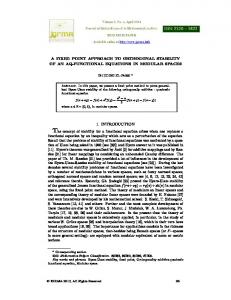
In the classic PTD algorithm, the parameter of grid cell size w, for seed point selection has In the classic algorithm,results. the parameter of grid size 1, , w forshould seed point selection a a significant effect onPTD the filtering As shown in cell Figure typically be has set larger significant effect on the filtering results. As shown in Figure 1, should typically be set larger than than the maximum building size to avoid selecting seed points on the roof of buildings. However, the maximum building size to avoid selecting seed points on the roof of buildings. However, given given that the lowest point in the grid is selected as the seed point, the selected seed points hardly that the lowest point in the grid is selected as the seed point, the selected seed points hardly appear appear in the vicinity of the mountain ridge. Thus, completely preserving the real terrain at the ridge in the vicinity of the mountain ridge. Thus, completely preserving the real terrain at the ridge could couldbebedifficult difficult during the subsequent TIN densification process. If some near theberidge during the subsequent TIN densification process. If some points near points the ridge could coulddetected be detected and used as additional seed points, the filtering results for mountainous areas and used as additional seed points, the filtering results for mountainous areas will will be improved. be improved.

Figure 1. Seed point selection forfora asteep areawith withbuildings buildings nearby. terrain Figure 1. Seed point selection steepmountainous mountainous area nearby. TheThe real real terrain and and the corresponding point cloud are separately drawn in two parts. In part (a), the buildings, trees, and and the corresponding point cloud are separately drawn in two parts. In part (a), the buildings, trees, topography are indicated with different colors. In part (b), the cyan dashed line defines the grid cell topography are indicated with different colors; In part (b), the cyan dashed line defines the gridfor cell for seed point selection; small red diamondshape shape represents represents the point selected as seed pointpoint in in seed point selection; thethe small red diamond thelowest lowest point selected as seed each grid, and the brown dashed line represents the initial terrain constructed with the seed points. each grid, and the brown dashed line represents the initial terrain constructed with the seed points.

On the basis of the sparse TIN structure constructed with the initial seed points, a rule-based

On the basis of the method sparse TIN structure with the initial seed points, a rule-based ridge point detection is designed. Theconstructed main idea of this method is to detect the triangles that ridgeare point detection method is designed. The main idea this method is tocenter detectofthe likely to be located on the ridge. Within a certain rangeofaround the gravity thetriangles triangle, that the lowest point is on selected as an Within additional seed point. our approach, this type of of triangle is are likely to be located the ridge. a certain rangeInaround the gravity center the triangle, referred to as the “ridge triangle,” which can be determined according to the following assumptions: the lowest point is selected as an additional seed point. In our approach, this type of triangle is referred to as (1) the “ridge triangle”,trend which canopposite be determined according to thetofollowing assumptions: The descending on the sides of the ridge. Owing this feature, Figure 1b shows (1)

that the distance between the seed points at the ridge is apparently longer. Compared with

The others, descending trend on the opposite sides of the ridge. Owing to this feature, Figure 1b shows the horizontal component ∆ of this distance could be closer to 2 . Thus, the ∆ values that for thethe distance between seed points is apparently Compared others, three sides of thethe judging triangleatinthe theridge TIN are calculated. longer. If at least one ∆ is with greater the horizontal component ∆ l of this distance could be closer to 2 w. Thus, the ∆l values for than the threshold , the triangle can be inferred as a potential ridge triangle. In our approach, the three sides the judging in the TIN calculated. If at least onea∆l is greater is theofproduct of thetriangle coefficient and are , with generally having value close tothan 2. the Considering the topographical trendas ofathe ridge can be represented along X-axis orlYthreshold lr , thethat triangle can be inferred potential ridge triangle. In ourthe approach, r is the axis of direction, ∆ can be using following equation: product the coefficient mrcalculated and w, with mrthe generally having a value close to 2. Considering that the topographical trend of the ridge be represented the X-axis or Y-axis direction, ∆l |} (1) ∆ = can max{| − |, | − along can be calculated using the following equation:

where

(2)

and

are the space coordinates of the triangle vertices.

(2) The convex slope inversion constraint. Thet|X main |u assumption is that the slope (1) ∆l “ max X2 | , |Y1 ´ of Y2this 1 ímplication changes dramatically at the ridge, as proposed in the earlier literature for ridge point extraction from DTM In the TINcoordinates structure constructed with sparse seed points, the changing trend Yi [50]. are the space of the triangle vertices. where Xi aand of the slope is retained even if the topographic feature of the ridge hasassumption weakened. According The convex slope inversion constraint. The main implication of this is that thetoslope this trend, the potential ridge triangle can be extracted from the TIN by calculating the dihedral changes dramatically at the ridge, as proposed in the earlier literature for ridge point extraction angle between the judging triangle and its adjacent triangles. The triangles that constitute a from a DTM [50]. In the TIN structure constructed with sparse seed points, the changing trend considerable angle with the ridge triangle should exist on both sides of the mountain. In our

of the slope is retained even if the topographic feature of the ridge has weakened. According to this trend, the potential ridge triangle can be extracted from the TIN by calculating the dihedral angle between the judging triangle and its adjacent triangles. The triangles that constitute


6 of 22

a considerable angle with the ridge triangle should exist on both sides of the mountain. In Remote Sens. 2016, 8,the 71 triangles connected to the directly adjacent triangles are also used 6 of 22 for the our approach, judgment considering that these three triangles may only include triangles on one side, as shown approach, the triangles connected to the directly adjacent triangles are also used for the in Figure 2. A triangle is generally determined as aonly ridge triangle if at twoastriangles in its considering that these three triangles may include triangles onleast one side, shown Remotejudgment Sens. 2016, 8, 71 6 of 22 vicinity fulfill the following conditions: (i) the dihedral angle between the judging triangle and in Figure 2. A triangle is generally determined as a ridge triangle if at least two triangles in its vicinity fulfill conditions: (i) dihedral angle between the judging triangle approach, thethe triangles connected thethe directly adjacent triangles are also used for and thetriangle the adjacent triangle isfollowing greater than thetothreshold θr ; (ii) the gravity center of the adjacent the adjacent triangle greater than triangles thetriangle; threshold ; (iii) (ii) the center the as adjacent judgment thesejudging three mayand only include triangles onpoint oneofside, shown is located belowconsidering the planeisthat of the no gravity common exists between the triangle is2.located below the planedetermined of the judging and (iii) common point exists in Figure A triangle is generally as a triangle; ridge triangle if atno least two triangles in its satisfied triangles. between the satisfied triangles. vicinity fulfill the following conditions: (i) the dihedral angle between the judging triangle and the adjacent triangle is greater than the threshold ; (ii) the gravity center of the adjacent triangle is located below the plane of the judging triangle; and (iii) no common point exists between the satisfied triangles.

Figure 2. Adjacent triangles for determining the ridge triangle. The green triangle represents the Figure 2. Adjacent triangles for determining the ridge triangle. The green triangle represents the judging triangle, the dark blue triangles represent the triangles directly adjacent to the judging judging triangle, the dark blue triangles represent the triangles directly adjacent to the judging triangle, triangle, and the light blue triangles represent the triangles connected to the directly adjacent triangles. and the light blue triangles represent the triangles connected to the directly adjacent triangles. Figure 2. Adjacent triangles for determining the ridge triangle. The green triangle represents the

In summary, when a triangle in the sparse TIN (1) to and it can be judging triangle, the dark blue triangles represent thesatisfies trianglesAssumptions directly adjacent the(2), judging detected as awhen ridge general, the terrain is usually not flat at the ridge, which means thatdetected triangle, and theatriangle. light blue In triangles the triangles connected to the directly In summary, triangle in the represent sparse TIN satisfies Assumptions (1) adjacent and (2),triangles. it can be large artificial objects rarely exist therein. Therefore, in our approach, the lowest point within a radius as a ridge triangle. In general, the terrain is usually not flat at the ridge, which means that large of 2 m the gravity of the in triangle is selected the ridge point. Figure shows Infrom summary, whencenter a triangle the sparse TIN as satisfies Assumptions (1)3and (2),the it results can be artificialofobjects rarelydetection exist therein. Therefore, in ourdatasets approach, the lowestFigure point3a,b within a radius of the ridge of thethe experimental in our illustrate detected as point a ridge triangle.for Inone general, terrain is usually not flat approach. at the ridge, which means that 2 m from theartificial gravity center of the triangle is selected the ridge point. Figure 3within shows the results of obvious gaps along the ridge line; these gaps are clearly caused by the descending trend of the ridge large objects rarely exist therein. Therefore, inas our approach, the lowest point a radius the ridge detection forcenter one the experimental in our approach. Figure illustrate terrain. Figure show that,of inthe most of the isgaps, thedatasets potential ridge points can 3beshows detected by the of point 2 m from the3c,d gravity of triangle selected as the ridge point. Figure the3a,b results method. Figure that the terrain surface constructed the initial seed points ofgaps the ridge point forindicate one of the experimental datasets in our Figure 3a,b illustrate obviousproposed along thedetection ridge 3e,f line; these gaps are clearly caused byapproach. thewith descending trend of the ridge the ridge preserves the these topographic features precisely. obvious gaps along ridge are clearly caused by the descending trendbe of detected the ridge by the terrain.and Figure 3c,dpoints showthe that, inline; most of gaps the gaps, the more potential ridge points can terrain. Figure 3c,d show that, in most of the gaps, the potential ridge points can be detected by the proposed method. Figure 3e,f indicate that the terrain surface constructed with the initial seed points proposed method. Figure 3e,f indicate that the terrain surface constructed with the initial seed points and theand ridge points preserves the topographic features more precisely. the ridge points preserves the topographic features more precisely.

Figure 3. Cont.

Figure 3. Cont.

Figure 3. Cont.


7 of 22


7 of 22

Figure 3. Results of ridge point detection. (a) Initial seed points selected from the stereo-matched point

Figure 3. Results of ridge point detection. (a) Initial seed points selected from the stereo-matched point cloud that are colored according to their elevations; (b) Enlarged view of the rectangular area in (a); (c) cloud that arepoints colored according (b)Enlarged Enlarged the rectangular Ridge detected based on to thetheir initialelevations; seed points; (d) viewview of the of rectangular area in (c);area (e), in (a); (c) Ridge based on theconstructed initial seed points; (d) Enlarged view of the rectangular area in (f)points Verticaldetected views of the TIN surfaces using the points in (b,d), respectively. (c); (e,f) Vertical views of the TIN surfaces constructed using the points in (b,d), respectively. 2.2. Optimal Selection of Seed Points inevitably included in the potential ridge points. For example, in the lower 2.2. OptimalErroneous Selection points of Seedare Points right area of Figure 3c, a few ridge points may be erroneously detected. Meanwhile, in the application

Erroneous points are inevitably included in the potential points. For example, the lower of the PTD algorithm for steep mountainous terrains, one of theridge essential requisites to achieve in good right area of Figure a few ridge may be erroneously the application results is to set3c, a relatively smallpoints . When drops to a certaindetected. size, errorsMeanwhile, would appearin among the initial seed points insteep residential areas. Thus,terrains, an optimal selection method of requisites seed pointsto based on good of the PTD algorithm for mountainous one of the essential achieve confidence interval estimation theory is proposed in our approach to eliminate the errors from the results is to set a relatively small w. When w drops to a certain size, errors would appear among the initial seed points and the ridge points. initial seed points in residential areas. Thus, an optimal selection method of seed points based on A small range of topographic surface can generally be well fitted using a conicoid model. When confidence interval estimation theory is proposed in our approach to eliminate errors as from the the model is estimated by seed points within a local area, while treating the point the elevations initial seed points and the ridge observations, gross errors canpoints. be detected according to their residuals. confidence interval theory,be thewell confidence intervals corresponding to When A smallAccording range oftotopographic surfaceestimation can generally fitted using a conicoid model. residuals can be estimated detect gross errors by judging the residual within the the model is estimated by seedto points within a local area, whether while treating thefalls point elevations as corresponding confidence interval. The details are as follows. observations, gross errors can be detected according to their residuals. In a local conicoid model, local seed points satisfy the following equation: According to confidence interval estimation theory, the confidence intervals corresponding to (2) = by+judging whether the residual falls within residuals can be estimated to detect gross errors the where confidence is the elevation vectorThe of the points, is follows. the unsolved parameter vector, and is the corresponding interval. details are as coefficient constructed the corresponding plane coordinates, as shown by In acorresponding local conicoid model,matrix local seed pointsbysatisfy the following equation: Equation (3):

(2) 1 Y “ Xβ ` ε 1 = (3) ⋮ ⋮ ⋮β is⋮ the ⋮unsolved ⋮ where Y is the elevation vector of the points, parameter vector, and X is the 1

corresponding coefficient matrix constructed by the corresponding plane coordinates, as shown by and are the plane coordinates of the -th seed point where and Equation (3): is the number of seed points » fi ( = 1,2, ⋯ , ). 1 x1 y1 x12 x1 y1 y21 In Equation (2), obeys the following multivariate normal distribution: — ffi — 1 x2 y2 x22 x2 y2 y22 ffi (4) ~ (0, ) X“— (3) .. .. .. .. .. ffi — .. ffi – . . . . . . fl where = and is the weight matrix, which 2is an identity2matrix in our approach. 1 xnthe yparameter yn be estimated as follows: n xn xvector n yn can According to the least square method,

where n is the number of seed points and x=i and yi) are the plane coordinates of the i-th seed point (5) ( (i “ 1, 2, ¨ ¨ ¨ Furthermore, , n). in confidence interval estimation, normalized residuals should be solved using a In Equation ε obeys multivariate normal distribution: covariance (2), matrix, whichthe canfollowing be estimated by the following equation: =

− (

ε „ Np0, Σq

)

(6)

(4)

The residual for every seed point can be obtained as follows:

where Σ “ σ02 P´1 and P is the weight matrix, which is an identity matrix in our approach. According to the least square method, the parameter vector can be estimated as follows: ´1 βˆ “ pX T PXq X T PY

(5)

Furthermore, in confidence interval estimation, normalized residuals should be solved using a covariance matrix, which can be estimated by the following equation:


8 of 22

´1 QVˆ Vˆ “ P´1 ´ XpX T PXq X T

(6)

The residual for every seed point can be obtained as follows: vî “ Xi βˆ ´ Yi

(7)

where vî is the estimated residual for the i-th point and Yi is the corresponding observed elevation. Sens. 2016, 8, 71 8 of 22 The Remote normalized residuals can be considered statistics that obey the following t distribution: ti “

vî = „− tnú´1 ? ˆσ0 qii

(7)

where is the estimated residual for the -th point and is the corresponding observed elevation. ˆ qii is the element of the can diagonal of QVˆstatistics and σ the unit weighteddistribution: RMSE calculated Thei-th normalized residuals be considered that the following ˆ 0 isobey V

where the following expression:

=

σˆ 0 “

d ř∼ n

is the -th element of the diagonal of where by the following expression:

2 i“0 vˆ i

(8) by

(8)

n ´ and u ´ 1 is the unit weighted RMSE calculated

(9)

where n is the number of observations and u is the parameter number of Equation (2). Given a confidence level of 1 ´ α (confidence probability), the corresponding confidence intervals ∑ (9) = − −1 pt, tq of the normalized residuals can be estimated according to the t distribution. In other words, the statistic twhere the following inequation: i shouldissatisfy the number of observations and is the parameter number of Equation (2). Given a confidence level of 1 − α (confidence probability), the corresponding confidence t ă ti ă t (10) intervals ( , ) of the normalized residuals can be estimated according to the distribution. In other should satisfy the following inequation: words, the statistic Thus, if ti does not fall in the confidence interval, then the corresponding point can be considered

a gross error. < < (10) The seedThus, points can be judged one by one on the basis of the preceding analysis. does not fall in the confidence interval, then the corresponding point canEvery be time a if point is judged, thea gross neighboring points are gathered. If the residual of the judging point cannot pass considered error. The test, seed points can be one by one on the the preceding Every time a can be the significance the point is judged eliminated. Using thebasis TINofstructure, theanalysis. neighboring points point is judged, the neighboring points are gathered. If the residual of the judging point cannot pass determined by an iterative method [51]: all the points adjacently connected to the judging point are the significance test, the point is eliminated. Using the TIN structure, the neighboring points can be first collected; more points that are adjacently connected to the collected points are then identified and determined by an iterative method [51]: all the points adjacently connected to the judging point are gathered first continually. In our approach, the recommended number 2.then identified collected; more points that are adjacently connected toiteration the collected pointsisare A major effect ofcontinually. the optimized for recommended seed points is that the grid is cell and gathered In our selection approach, the iteration number 2. size w can be assigned A major effect of thetooptimized selection for seed points is that the gridbe cell canofbethe value to a larger range. According the authors’ experience, w can generally setsize to half assigned to a larger range. According to the authors’ experience, can generally be set to half of the adopted in the classic PTD algorithm. Figure 4 shows the optimal selected results of the seed points. value adopted in the classic PTD algorithm. Figure 4 shows the optimal selected results of the seed After optimization, the gross errors among the initial seed points and the ridge points are both well points. After optimization, the gross errors among the initial seed points and the ridge points are both eliminated, whereas most of the additional ridgeridge points areare preserved. well eliminated, whereas most of the additional points preserved.

Figure 4. Cont.

Figure 4. Cont.

Remote Sens.2016, 2016,8,8,7171 Remote Sens. Remote Sens. 2016, 8, 71

9 of 22 9 of 22

Figure 4. Triangulated irregular network (TIN) surfaces constructed with seed points before and after

Figure 4. Triangulated irregular network (TIN) surfaces constructed with seed points before and after optimal selection. irregular (a) Results network of the initial seed surfaces points; (b)constructed Results of the seed points after adding theand after Figure selection. 4. Triangulated seedpoints points before optimal (a) Results of the initial (TIN) seed points; (b) Results ofwith the seed after adding the detected ridge points; (c) Results of the seed points after optimal selection. The yellow ellipses indicate optimal selection. (a) Results of the initial seed points; (b) Results of the seed points after adding the detected ridge points; Results the seed points optimal The yellow ellipses the areas where(c) gross errors of among the initial seedafter points appear, selection. and the black ellipses indicate the indicate detected ridge points; (c) Results of the seed points after optimal selection. The yellow ellipses indicate where gross errorsamong among additional ridge points appear. the areasareas where gross errors the initial seed points appear, and the black ellipses indicate the the areas among the initial points appear, and the black ellipses indicate the areas wherewhere grossgross errorserrors among additional ridgeseed points appear. 2.3.where A Memory-Efficient Densification Strategy areas gross errorsTIN among additional ridge points appear. During the filtering process for the point clouds with high density, computational efficiency and 2.3. A Memory-Efficient TIN Densification Strategy 2.3. A Memory-Efficient TINare Densification Strategyin the implementation of the PTD algorithm. In our memory consumption significant problems approach, the matching resultfor obtained by SGM can be a point with computational very high density.efficiency During the filtering process the point clouds with highcloud density, During the filtering process for therequires point clouds withmemory, high density, computational efficiency and Considering that TIN construction significant sufficient memory to process and memory consumption are significant problems in the implementation of the PTD algorithm. In memoryexcessive consumption are be significant the implementation of the PTD algorithm. points may difficult toproblems achieve. Ininpractical applications, a point cloud with a large In our our approach, the matching result obtained by SGM can be a point cloud with very high density. number points is often divided into square or subsampled a lower density before filtering. approach, the ofmatching result obtained by tiles SGM can be a into point cloud with very high density. Considering that TIN construction significant memory, sufficient memory to process excessive However, the datarequires mayrequires result in the “border effect” [30], andsufficient some topographic details Considering thatpartitioning TIN construction significant memory, memory to process points may to In practical applications, point cloud large number of maybe be difficult lost because ofachieve. subsampling, causing missed detection ofaterrain points in with certainasituations. excessive points may be difficult to achieve. In practical applications, a point cloud with a large For example, the original point data (in Figure 5a) are subsampled by keeping the lowest point in the points is often divided intodivided square into tilessquare or subsampled into a lower density before filtering. number of points is often tiles or subsampled into a lower density beforeHowever, filtering. grid cell (in Figure 5b). If the threshold of the maximum distance for TIN densification is valued partitioning the data may result in the “border effect” [30], and some topographic details maydetails be lost However, partitioning the data may result in the “border effect” [30], and some topographic between and , then terrain point will not be detected. because of subsampling, causing missed detection of terrain points in certain situations. For example, may be lost because of subsampling, causing missed detection of terrain points in certain situations. the point (in Figure 5a) (in areFigure subsampled keeping the in the point grid cell (in Fororiginal example, the data original point data 5a) are by subsampled by lowest keepingpoint the lowest in the Figure 5b). If the threshold of the maximum distance for TIN densification is valued between d and A grid cell (in Figure 5b). If the threshold of the maximum distance for TIN densification is valued d Bbetween , then terrainand point ,Pthen not bepoint detected.will not be detected. A will terrain

Figure 5. Example of TIN densification in a local area. The brown line represents the actual terrain, and the blue dashed line represents the TIN surface constructed with the detected terrain points. The red diamond shapes represent the points labeled as terrain points, and the white diamonds represent the points labeled as off-terrain points. (a) Sectional view of the original point cloud, where and are the distances from and to the corresponding triangle, respectively, and is the grid cell size for determining the lowest point; (b) cannot be labeled as a terrain point if the points are subsampled in advance; (c,d) Densification results using the proposed strategy in two iterations, is successfully labeled. where

Figure5.5.Example ExampleofofTIN TINdensification densification in in aalocal local area. area. The The brown brown line Figure line represents represents the the actual actual terrain, terrain, and the blue dashed line represents the TIN surface constructed with the detected terrain points. and the blue dashed line represents the TIN surface constructed with the detected terrain points. The The reddiamond diamondshapes shapesrepresent representthe thepoints pointslabeled labeledas asterrain terrain points, points, and and the the white red white diamonds diamonds represent represent thepoints pointslabeled labeledasasoff-terrain off-terrainpoints. points. (a) (a) Sectional Sectional view view of the of the the original original point pointcloud, cloud,where where d A and and are the distances from and to the corresponding triangle, respectively, and is the d B are the distances from PA and PB to the corresponding triangle, respectively, and m is the grid grid cellsize sizefor fordetermining determiningthe thelowest lowestpoint; point; (b) (b) P cannot cannotbe belabeled labeled as as aa terrain terrain point point if cell if the the points points are are A subsampled in advance; (c,d) Densification results using the proposed strategy in two iterations, subsampled in advance; (c,d) Densification results using the proposed strategy in two iterations, where is successfully PAwhere is successfully labeled. labeled.


10 of 22

A memory-efficient TIN densification strategy for high-density point clouds is adopted to address the aforementioned problems. This strategy was proposed in our previous work [49] and can be summarized in the following steps: (1) (2) (3)

(4)

(5)

The optimized seed points are all labeled as terrain points. A TIN is constructed using terrain points. All the off-terrain points are judged one by one. The distance and angles are calculated for the judging point and its corresponding triangle. The point is then labeled as a terrain point if the threshold condition is satisfied. After traversing all the off-terrain points, the total number of i current terrain points, Nground is recorded, where i represents the iteration rounds. A grid with cell size m is created, and all grid cells are then traversed. If a grid cell has terrain points in it, then only the lowest terrain point is retained, whereas all the other terrain points are relabeled as off-terrain points. The value of m can be determined according to the resolution of the final acquired DTM. Steps (2) to (4) are repeated. In step (3), the proportion of the increased terrain points in the total points is calculated as follows: i ´1 i p “ pNground ´ Nground q{Ntotal

(11)

When p is larger than the threshold pmin the following step is performed; otherwise, the loop ends. In our approach, pmin is set to 0.001. Through this strategy, instead of subsampling the point cloud before filtering, the points presenting a more detailed topography are preserved. Therefore, the rejection of terrain points can be avoided in some situations when using the same parameters. As shown in Figure 5c,d, PA can be successfully labeled as a terrain point in our approach using the same distance threshold between d A and d B . In this strategy, only the lowest points in the grid cells are used to construct a TIN during the densification process. Thus, the number of points for TIN construction is controlled, and the memory consumption is reduced. Specifically, the theoretical maximum number of points for TIN construction can be limited to: Nmax “ W ¨ H{m2 (12) where W and H represent the width and height of the bounding rectangle of the point cloud data, respectively; m is the grid cell size aforementioned. 3. Experiments and Results 3.1. Testing Data The testing data used in the experiments are obtained from Shaoguan, a southern city in the Guangdong Province of China. The main terrain in Shaoguan is mountainous, but many residential areas also exist in the city. The aerial images are captured using a Digital Mapping Camera with a focal length of 92 mm at 3600 m altitude. The forward overlap of images is 65%, and the size of each image is 14,144 ˆ 15,552 pixels with a spatial resolution of 0.2 m. Two sets of point clouds matched from two consecutive stereo image pairs are used for the experiments. The maximum elevation differences in the two datasets are more than 300 m. Each of the point cloud dataset covers an area of approximately 3100 ˆ 1800 m2 . The target of this study is to generate DTMs with grid size of 1 m; thus, in order to avoid processing excessively redundant data, the matching results are subsampled into one-half of the original resolution. The point density of the subsampled point cloud is 6 points/m2 , and the total number of points for each dataset is over 12 million. In the datasets, eight sites are selected to evaluate the filtering results, including four residential sites and four mountainous sites. Figure 6 shows the experimental and evaluation areas in the


11 of 22

coordinate system of the 1984 World Geodetic System. Given that the ground truth data are unavailable Remote Sens. 2016, 8, 71 11 of 22 in the testing area, TerraScan software is adopted to classify the points of each site into terrain and off-terrain by careful manual editing. obtained ground points are are interpolated terrainpoints and off-terrain points by careful manualThe editing. The obtained ground points interpolatedinto a into a regular-grid DTM, is then as a reference regular-grid DTM, which is which then used as used a reference DTM.DTM.

Figure 6. Experimental and evaluation areas. (a,b) TIN surfaces constructed with the point clouds of Figure 6. Experimental and evaluation areas. (a,b) TIN surfaces constructed with the point clouds the two datasets, which are colored based on the texture of the aerial images. The red rectangles of the two datasets, which are colored based on the texture of the aerial images. The red rectangles indicate the areas for DTM accuracy evaluation of the residential areas, and the yellow rectangles indicate the areas for DTM accuracy evaluation of the residential areas, and the yellow rectangles indicate the areas for evaluating mountainous areas. indicate the areas for evaluating mountainous areas.

3.2. Evaluation and Comparison

3.2. Evaluation and Comparison

The proposed algorithms are implemented using C++ language. In seed point optimization, the

confidence interval must be are obtained from the using t distribution table according the confidence The proposed algorithms implemented C++ language. In seedtopoint optimization, probability.interval This process accomplished using the GNU Scientific to Library [52]. the confidence mustisbeautomatically obtained from the t distribution table according the confidence A desktop computer with a 64-bit Windows 7 operating system, a quad-core Intel Core i5-3470 CPU, probability. This process is automatically accomplished using the GNU Scientific Library [52]. 3.2 GHz, and 4 GB memory is utilized for the experiments. Given that the proposed approach is an A desktop computer with a 64-bit Windows 7 operating system, a quad-core Intel Core i5-3470 improved PTD method, the implementation of the classic PTD method in the TerraScan software CPU,package 3.2 GHz, and 4 GB memory is utilized for the experiments. Given that the proposed approach is is used for comparison. Meanwhile, three other filtering algorithms including progressive an improved PTD method, the implementation of the PTD method(LP) in the software morphology (PM) [20], multiscale curvature (MC) [27] classic and linear prediction [26]TerraScan are also tested package is used for comparison. Meanwhile, three other filtering algorithms including progressive in our experiment. These three methods are implemented in the free softwares of ALDPAT [53], morphology (PM)[54] [20], multiscale curvature (MC) [27] and linear prediction (LP) [26] are also tested MCC-LIDAR and FUSION [55], respectively. Table 1 shows the three main parameters used by the proposed method. The first five [53], in our experiment. These methods are implemented in thefiltering free softwares of ALDPAT parameters are shared by the classic PTD algorithm and the proposed algorithm and are set to the MCC-LIDAR [54] and FUSION [55], respectively. same values across the experiments. The detailed meanings of these parameters are given in [35]. The five Table 1 shows the main parameters used by the proposed filtering method. The first last three parameters are the additional parameters in our approach. Parameters for the proposed parameters are shared by the classic PTD algorithm and the proposed algorithm and are set to method and all the compared methods are tuned for maximum performance. However, it should be the same values across the experiments. The detailed meanings of these parameters are given in [35]. noted that the datasets with two types of terrains are processed with equivalent parameters. The most The last three parameters are the additional parameters in our approach. Parameters for the proposed important criterion for parameter selection is to balance the filtering results between the residential method all the compared methods are tuned for maximum performance. However, it should be andand mountainous areas. noted that the datasets with two types of terrains are processed with equivalent parameters. The most important criterion for parameter selection is to balance the filtering results between the residential and mountainous areas.


12 of 22

Table 1. Main parameters of the proposed method. Parameters

Values

Grid cell size w Maximum terrain angle t Maximum angle θ Maximum distance d Minimum edge length l Minimum times of edge length in ridge mr Minimum angle in ridge θr Confidence probability 1 ´ α

20 m 88.0˝ 6.0˝ 1.4 m 1m 1.5 25 98%

Given that this study aims to generate high-quality DTM data, the ground points obtained by filtering algorithms are interpolated into DTMs for evaluation. The elevation discrepancies between the generated and the reference DTMs are computed, and the RMSEs calculated from these discrepancies are used to quantify the accuracy of the generated DTM [56]. Apart from the calculation of RMSE for every single site, the overall accuracy values for all residential and mountainous sites respectively represented by RMSEr and RMSEm are calculated for each dataset. The total accuracy RMSEtotal for each dataset is also calculated based on the statistics of points for all the sites. Tables 2 and 3 list the RMSE values for the eight sites in the two datasets, where RMSEi represents the RMSE value for Site i. For residential areas, the DTM of the proposed method achieved the highest accuracy value among the five compared methods. For mountainous areas, MC and LP generated the best results in Dataset 1 and 2, respectively, with the proposed method following by a slight difference. For total areas, the proposed method is obviously better than the other methods. Therefore, when using the same set of parameters for filtering, the proposed method can achieve relatively high accuracy values for both residential and mountainous areas. Table 2. Comparison of the RMSE results (in meters) for Dataset 1. Method

RMSE1

RMSE2

RMSEr

RMSE3

RMSE4

RMSEm

RMSEtotal

PM MC LP PTD Proposed

1.022 0.860 1.431 0.440 0.455

1.381 1.296 1.638 0.742 0.359

1.266 1.161 1.568 0.651 0.396

1.652 1.309 1.348 1.750 1.461

1.085 0.965 1.066 1.509 0.960

1.423 1.165 1.228 1.645 1.259

1.353 1.163 1.395 1.286 0.963

Table 3. Comparison of the RMSE results (in meters) for Dataset 2. Method

RMSE5

RMSE6

RMSEr

RMSE7

RMSE8

RMSEm

RMSEtotal

PM MC LP PTD Proposed

1.340 1.296 1.761 0.552 0.591

1.690 1.633 2.044 0.904 0.603

1.486 1.437 1.876 0.710 0.596

1.445 1.349 1.298 1.601 1.271

2.032 1.090 1.047 1.715 1.215

1.709 1.250 1.202 1.649 1.249

1.612 1.338 1.544 1.309 1.007

Among the filtering results, we select a mountain site and a residential site from the two datasets to perform a visual evaluation. The selected sites include Sites 1, 4, 6, and 7. Figures 7–10 show the comparative results of the generated DTMs for these sites. Figures 7 and 9 indicate that the problems of PM, MC and LP lie in the acceptance of obvious objects as terrains. Figures 8 and 10 indicate that more points near the mountain ridge are rejected by PM and PTD. The proposed method achieves a better overall performance on the two different types of terrain.


13 of 22


13 of 22


13 of 22

Figure 7. TIN surfaces constructed with the points of Site 1 and its filtering results. (a) Original stereo-

Figure 7. TIN surfaces constructed withobtained the points Site 1editing; and its(c–g) filtering results. Original matched point cloud; (b) Reference DTM fromof manual Filtering results (a) of PM, Figure 7. TIN surfaces constructed with the points of Site 1 from and itsmanual filteringediting; results. (a) Original stereostereo-matched cloud; (b) Reference DTM obtained (c–g) Filtering results MC, LP, PTDpoint and the proposed method, respectively. matched point cloud; (b) Reference DTM obtained from manual editing; (c–g) Filtering results of PM, of PM, MC, LP, PTD and the proposed method, respectively. MC, LP, PTD and the proposed method, respectively.

Figure 8. Cont. Figure 8. Cont.

Figure 8. Cont.

Remote Sens. 2016, 8, 71 Remote Sens. 2016, 8, 71 Remote Sens. 2016, 8, 71

14 of 22 14 of 22 14 of 22

Figure 8. Orthographs of TIN surfaces of Site 4 and its filtering results. (a) Original stereo-matched

Figure 8. Orthographs of of TIN TIN surfaces surfaces of of Site Site 44 and filtering results. (a) Original stereo-matched Figure 8. Orthographs and its itsediting; filtering results. (a)results Original stereo-matched point cloud; (b) Reference DTM obtained from manual (c–g) Filtering of PM, MC, LP, point cloud; (b) Reference DTM obtained from manual editing; (c–g) Filtering results ofPM, PM,MC, MC,LP, LP, pointPTD cloud; (b) Reference DTM obtained from manual editing; (c–g) Filtering results and the proposed method, respectively. The white ellipses indicate the areas whereof the terrain PTD and the proposed method, respectively. The white ellipses indicate the areas where the terrain near the ridgemethod, are obviously rejected during the filtering process. PTD points and the proposed respectively. The white ellipses indicate the areas where the terrain points near the ridge are obviously rejected during the filtering process. points near the ridge are obviously rejected during the filtering process.

Figure 9. TIN surfaces constructed with the points of Site 6 and its filtering results. (a) Original stereo-matched point cloud; (b) Reference DTM obtained from manual editing; (c–g) Filtering results of PM, MC, LP, PTD and the proposed method, respectively.

Figure 9. TIN Site 66 and and its its filtering filtering results. results. (a) (a) Original Original Figure 9. TIN surfaces surfaces constructed constructed with with the the points points of of Site stereo-matched stereo-matched point point cloud; cloud; (b) (b) Reference Reference DTM DTM obtained obtained from from manual manual editing; editing; (c–g) (c–g) Filtering Filtering results results of PM, MC, LP, PTD and the proposed method, respectively. of PM, MC, LP, PTD and the proposed method, respectively.


15 of 22


15 of 22

Figure 10. Cont. Figure 10. Cont.



16 of 22

16 of 22

Figure 10. Orthographs of TIN surfaces of Site 7 and its filtering results. (a) Original stereo-matched Figure 10. Orthographs of TIN surfaces of Site 7 and its filtering results. (a) Original stereo-matched point cloud; (b) Reference DTM obtained from manual editing; (c–g) Filtering results of PM, MC, LP, point cloud; (b) Reference DTM obtained from manual editing; (c–g) Filtering results of PM, MC, LP, PTD and the proposed method, respectively. The white ellipses indicate the areas where the terrain PTD and the proposed method, respectively. The white ellipses indicate the areas where the terrain points near the ridge are obviously rejected during the filtering process. points near the ridge are obviously rejected during the filtering process.

The processing times of PM, MC, LP, PTD and the proposed method are 198, 600, 43, 110 and times of PM, LP,and PTD115 ands the proposed are 198, 600,be 43,seen 110 and 111 sThe for processing Dataset 1 and 205, 660, MC, 47, 103 for Dataset 2,method respectively. It can that 111 the sspeed for Dataset 1 and 205, 660, 47, 103 and 115 s for Dataset 2, respectively. It can be seen that the speed of of the proposed method is very close to that of the classic PTD. The efficiency of the proposed the proposed method is very close to that of the classic PTD. The efficiency of the proposed approach approach should be acceptable for most general applications. should be acceptable for most general applications. 4. Discussion 4. Discussion 4.1. Main Features of the Proposed Method 4.1. Main Features of the Proposed Method Some improvements on the classic PTD algorithm are proposed in this study. The improved Some improvements on the classic PTD algorithm are proposed in this study. The improved method is successfully applied to DTM generation using the point cloud derived from stereo aerial method is successfully applied to DTM generation using the point cloud derived from stereo aerial images. The main advantage of the proposed approach is the generation of relatively good filtering images. The main advantage of the proposed approach is the generation of relatively good filtering results for both residential areas and mountainous terrains with the use of the same set of parameters. results for both residential areas and mountainous terrains with the use of the same set of parameters. Many of other filtering methods use different parameters when dealing with different Many of other filtering methods use different parameters when dealing with different terrains [18,29,35,36]. Some experiments confirm that better results can be obtained with optimized terrains [18,29,35,36]. Some experiments confirm that better results can be obtained with optimized parameters than single parameters [22]. It means that in such methods, when the data include both parameters than single parameters [22]. It means that in such methods, when the data include both residential and mountainous areas, the two different terrains are preferably to be segmented to obtain residential and mountainous areas, the two different terrains are preferably to be segmented to obtain better filtering results. However, this process usually requires manual intervention and can be time better filtering results. However, this process usually requires manual intervention and can be time consuming. By contrast, the proposed method can achieve good results without data segmentation, consuming. By contrast, the proposed method can achieve good results without data segmentation, thereby considerably improving the applicability and automation degree of the PTD algorithm. thereby considerably improving the applicability and automation degree of the PTD algorithm. Most of the previous works have adopted the LiDAR data provided by the International Society Most of the previous works have adopted the LiDAR data provided by the International Society for Photogrammetry and Remote Sensing (ISPRS) for evaluation and comparison [11]. This study for Photogrammetry and Remote Sensing (ISPRS) for evaluation and comparison [11]. This study focuses more on validating the feasibility of generating DTM with stereo-matched point cloud; hence, focuses more on validating the feasibility of generating DTM with stereo-matched point cloud; hence, the ISPRS benchmark datasets are not used in our approach. The other feature of our approach is the the ISPRS benchmark datasets are not used in our approach. The other feature of our approach is high-density and steep slope of the processed point cloud data. The maximum height difference in our the high-density and steep slope of the processed point cloud data. The maximum height difference experimental datasets is more than 300 m. In addition, there are some filtering methods particularly in our experimental datasets is more than 300 m. In addition, there are some filtering methods developed for mountainous terrains [19,27,30,31,48]; however, compared with our method, the particularly developed for mountainous terrains [19,27,30,31,48]; however, compared with our method, practicability of these methods for residential areas has not been demonstrated. the practicability of these methods for residential areas has not been demonstrated. 4.2. Sensitivity Analysis of the Parameters Among the eight main parameters defined in the proposed method, the first five parameters are shared with the classic PTD algorithm. Since TerraScan has been able to give the recommended values for these parameters that perform well in many applications, this study determines these


17 of 22

4.2. Sensitivity Analysis of the Parameters Among the eight main parameters defined in the proposed method, the first five parameters are shared with the classic PTD algorithm. Since TerraScan has been able to give the recommended values for these parameters that perform well in many applications, this study determines these parameters by fine tuning the values suggested from TerraScan. mr , θr , and α are three new parameters in our approach. These three parameters are determined according to their influence on the filtering results. Both mr and θr are used for ridge point detection. The influence of these two parameters can be generally concluded follows: when mr and θr decrease, the detected ridge points in17mountainous Remote Sens. 2016,as 8, 71 of 22 areas increase, but RMSEr or even RMSEtotal also increases. The reason is that the gradually increasing parameters by fine tuning the values suggested from TerraScan. , , and α are three new gross errors among the detected ridge points cannot be satisfactorily eliminated in the subsequent parameters in our approach. These three parameters are determined according to their influence on optimization Parameter usedare forused the for optimal selection of seed points; when the process. filtering results. Both α is and ridge point detection. The influence of thesethis twoparameter parameters can be generally concluded as follows: when and decrease, the detected ridge increases from 0, RMSEr decreases. However, when α increases to a certain value (larger than 0.05 in points the in mountainous areas increase, but or evenis significantly also increases. The reason issome local our approach), DTM accuracy for mountainous areas affected, because that the gradually increasing gross errors among the detected ridge points cannot be satisfactorily areas of the mountainous terrains cannot be precisely approximated with a conicoid model. The ridge eliminated in the subsequent optimization process. Parameter α is used for the optimal selection of points or even the initial points inincreases these areas may be erroneously removed. large seed points; whenseed this parameter from 0, decreases. However, when A α significantly increases a certain value (larger than 0.05adversely in our approach), DTM for accuracy for mountainous areas isonly a few α not onlytoincreases RMSE also affectsthe results residential areas because m , but significantly affected,after because some local areas of the mountainous terrains cannot be precisely seed points can be retained optimization. approximated with a conicoid model. The ridge points or even the initial seed points in these areas Among the five parameters of the classic PTD algorithm, the grid cell, but size, w, is the parameter may be erroneously removed. A significantly large α not only increases also adversely with an obvious effect on the final results. Multiple w values ranging from 10 m to 55 m are used to affects results for residential areas because only a few seed points can be retained after optimization. Among the five parameters of the classic PTD algorithm, the grid cell size, , is the parameterof the grid generate the filtering results of the two methods for Dataset 1 to investigate the influence with an obvious effect on the final results. Multiple values ranging from 10 m to 55 m are used to cell size on the classic PTD and the proposed method. As shown in Figure 11, for residential areas, generate the filtering results of the two methods for Dataset 1 to investigate the influence of the grid the DTM accuracy of PTD is apparently improved from 10 m to 35 m and becomes stable when w is cell size on the classic PTD and the proposed method. As shown in Figure 11, for residential areas, greater than m,accuracy whereas the accuracy ofimproved the proposed generally stable, exceptiswhen w is the35 DTM of PTD is apparently from 10method m to 35 misand becomes stable when greater than 35 m,areas, whereas theaccuracies accuracy of the proposed methodare is generally stable, when w, but the 10 m. For mountainous the of both methods reduced withexcept increasing is 10 m. For mountainous areas, the accuracies of both methods are reduced with increasing proposed method is less sensitive. Both methods achieve the highest accuracies when, but w is equal to the proposed method is less sensitive. Both methods achieve the highest accuracies when is equal 15 m because the buildings in Dataset 1 are generally small. to 15 m because the buildings in Dataset 1 are generally small.

Figure 11. DTM accuracy values obtained by PTD and the proposed method using different

values.

Figure 11. (a–c) DTM accuracy values obtained by PTD and the proposed method using different w values. Comparative results of , and respectively. (a–c) Comparative results of RMSEr , RMSEm and RMSEtotal respectively. 4.3. Accuracies, Errors, and Uncertainties thatand the Uncertainties ground truth data are unavailable, the manual filtering results are used as the 4.3. Accuracies,Given Errors, reference data in our approach. The comparative trials suggest that the DTM accuracy obtained by

Giventhethat the ground data arethose unavailable, the manual filtering areand used as the proposed methodtruth is better than of the comparative methods when results residential mountainous areas are contained in a single dataset. reference data in our approach. The comparative trials suggest that the DTM accuracy obtained by the In order to conduct further analysis the filtering accuracies of the testing methods, three proposed method is better than those of theoncomparative methods when residential andkinds mountainous of errors defined in [11], namely, type I errors (i.e., omission errors), type II errors (i.e., commission areas are contained in a single dataset. errors) and total errors are evaluated. The evaluation results in Figure 12 suggest that, for residential


18 of 22

In order to conduct further analysis on the filtering accuracies of the testing methods, three kinds of errors defined in [11], namely, type I errors (i.e., omission errors), type II errors (i.e., commission errors) and total errors are evaluated. The evaluation results in Figure 12 suggest that, for residential areas (Site 1, 2, 5 and 6), most of the testing methods have relatively low type I errors in our experiment. Remote 2016, 8, 71 I errors for all the four sites, the type I errors of the proposed method 18 ofrank 22 MC has theSens. lowest type 2nd at Site 1 and 5, and rank 4th and 3rd at Site 2 and 6, respectively. In the assessment of type II errors, areas (Site 1, 2, 5 and 6), most of the testing methods have relatively low type I errors in our PTD and the proposed method perform better than other methods, PTD ranks 1st at Site 1, 2 and 5, experiment. MC has the lowest type I errors for all the four sites, the type I errors of the proposed the proposed method 1st at Siterank 6. Meanwhile, methods also have total errors method rank 2nd atranks Site 1 and 5, and 4th and 3rd atthe Sitetwo 2 and 6, respectively. In thelower assessment than other PTDand ranks 1st at Sitemethod 1 and perform 2, the proposed method ranks 1st at ranks Site 51st and of typemethods. II errors, PTD the proposed better than other methods, PTD at 6. For Site 1, 2 and 5, the proposed at Site 6.method Meanwhile, two methods also have lower mountainous areas (Site 3, 4, 7method and 8),ranks the 1st proposed hasthe the lowest type I errors for all the methods. PTDIIranks 1stfor at Site 1 and 2, the method In ranks at Site sites, total but iterrors alsothan has other the highest type errors all the sites inproposed the meantime. the1st assessment of 5 and 6. For mountainous areas (Site 3, 4, 7 and 8), the proposed method has the lowest type I errors total errors, the proposed method can be considered as the best method, which ranks 3rd at Site 3, for all the sites, but it also has the highest type II errors for all the sites in the meantime. In the and ranks 1st at Site 4, 7 and 8, respectively. The second best method for mountainous area is MC, assessment of total errors, the proposed method can be considered as the best method, which ranks which ranks 2nd at all the four sites. It can be seen that the proposed method performs worse in the 3rd at Site 3, and ranks 1st at Site 4, 7 and 8, respectively. The second best method for mountainous assessment type II errors of type errors. However, considering thatmethod in the manual area is of MC, which ranks than 2nd atthat all the four Isites. It can be seen that the proposed performsediting process, theincost repairing II errors is significantly lower than that of repairing worse the of assessment of the typetype II errors than that of type I errors. However, considering that in the the type I errorsmanual [11], the proposed method should requirethe lesstype human intervention compared thethat other editing process, the cost of repairing II errors is significantly lower to than of filters. repairing the that type the I errors thedata proposed method require human intervention Considering point[11], cloud processed areshould obtained fromless stereo image matching, the the other filters. errorscompared of imagetomatching directly influence the quality of the final DTM. The dense matching for Considering that the point cloud data processed are obtained from stereo image matching, the stereo images is a complex issue. The matching result can be influenced by many factors, such as errors of image matching directly influence the quality of the final DTM. The dense matching for the precision of aerial triangulation adjustment, the lack of image texture, and the uneven brightness. stereo images is a complex issue. The matching result can be influenced by many factors, such as the However, the point cloud in our approach is generated SGM, which has demonstrated precision of aerial triangulation adjustment, the lack of by image texture, and thebeen uneven brightness. to be a stable algorithm on the practical processing of aerial image matching [9]. However, the point cloud in our approach is generated by SGM, which has been demonstrated to be When terrain is coupled with a forest cover, defining a DTM a stablesteep algorithm on the practical processing of aerial image matching [9]. becomes difficult because steep terrain coupled withasa terrains. forest cover, a DTM becomes because points on When low branches mayisbe mistaken Thedefining proposed method triesdifficult to prevent detecting points points on low branches mayinbetwo mistaken terrains. The proposed method tries to prevent detectinghigher vegetation as terrains ways.asFirst, if there are vegetation points with obvious vegetation points as terrains in two ways. First, if there are are vegetation points with obvious higher elevation that are wrongly selected as the ridge points, they likely to be removed as gross errors in elevation that are wrongly selected as the ridge points, they are likely to be removed as gross errors the subsequent optimization process. Moreover, the adopted TIN densification strategy can resist the in the subsequent optimization process. Moreover, the adopted TIN densification strategy can resist disturbance of vegetation points to a certain extent,extent, because onlyonly the lowest points in the grid cells are the disturbance of vegetation points to a certain because the lowest points in the grid used for TIN construction during the densification process. cells are used for TIN construction during the densification process.

Figure 12. Three types of errors of the comparative filtering methods for the eight testing sites. (a–c)

Figure 12. Three types of errors of the comparative filtering methods for the eight testing sites. (a–c) Type I errors, type II errors and total errors of the comparative methods for the testing sites, respectively. Type I errors, type II errors and total errors of the comparative methods for the testing sites, respectively.


19 of 22

Considering that the point cloud data processed are obtained from stereo image matching, the errors of image matching directly influence the quality of the final DTM. The dense matching for stereo images is a complex issue. The matching result can be influenced by many factors, such as the precision of aerial triangulation adjustment, the lack of image texture, and the uneven brightness. However, the point cloud in our approach is generated by SGM, which has been demonstrated to be a stable algorithm on the practical processing of aerial image matching [9]. Unlike airborne LiDAR data, the point cloud obtained from aerial photogrammetry can only define the upper canopy surface in forest areas with dense leaves, causing considerable uncertainty about the absolute accuracy of the generated DTM. However, the main topographic features are retained in the stereo-matched point cloud. Although the accuracy is affected by labeling some leaf points as terrain points, the obtained DTM remains useful for many practical applications, such as image rectification, floodplain mapping, and land erosion analysis. Currently, the improvement of the proposed method is verified using point cloud data derived from stereo images at only one location, thus the filtering results might vary for other different scenarios. The proposed method is mainly designed for DTM generation with high resolution (1 m), the experimental results show that it performs well for stereo-matched point cloud with 6 points/m2 density. However, in-depth experiments and analyses for LiDAR data have not been done in our works. Considering that compared with stereo-matched point cloud, LiDAR data may have lower density and represent a more complex spatial distribution, it should be pointed out that the applicability of the proposed method for LiDAR data remains uncertain. 5. Conclusions An improved progressive TIN (triangulated irregular networks) densification (PTD) algorithm is proposed for digital terrain model (DTM) generation with the point clouds derived from aerial image matching. Given that residential and mountainous areas are contained in a single dataset, this approach aims to achieve relatively high accuracy values for the two different terrains using the same set of parameters. The main improvements are as follows: first, a rule-based method for detecting ridge points is used to enhance filtering performance for steep mountainous terrains. The detected potential ridge points are used as additional seed points. Second, an optimal selection method based on confidence interval estimation theory is applied to seed points to eliminate the erroneous points among the potential ridge points and the initial seed points. A memory-efficient TIN densification strategy is also proposed to process high-density point clouds. In this strategy, the number of points for TIN construction is controlled, and some points presenting a detailed topography can be preserved. The experiments on two sets of stereo-matched point clouds with more than 12 million points indicate that the proposed method performs well both for mountainous and residential areas. The total accuracy values of the generated DTMs in the form of root-mean-square errors are 0.963 and 1.007 m, respectively, which are better than the 1.286 and 1.309 m achieved by the classic PTD method. The times consumed by the proposed method for the two datasets are 111 and 115 s, respectively, which are very close to those of the classic PTD method and can thus meet the requirements of most applications. However, the proposed approach mainly focuses on the overall accuracy for different types of terrain and in the process fails to provide an in-depth analysis of the filtering results for local areas. A subsequent study will investigate the problems encountered in detail, and the applicability of our method to point clouds obtained from airborne light detection and ranging will also be considered in the future. Acknowledgments: This research was supported by the National Natural Science Foundation of China with Project Number 41471355 and 41301519. We also thank Rongyong Huang, Shiyan Pang and Zhiqi Zuo for their support during the entire course of this study. Author Contributions: Q.C. and H.W. conceived the idea; H.Z. and X.L conducted the analysis; M.S. processed the data; all authors contributed to the writing and revisions. Conflicts of Interest: The authors declare no conflict of interest.


20 of 22

References 1. 2. 3. 4. 5. 6.

7.

8.

9. 10. 11. 12. 13. 14. 15. 16. 17.

18. 19. 20.

21.

22.

Miller, C.L.; Laflamme, R.A. The digital terrain model: Theory and application. Photogramm. Eng. 1958, 24, 433–442. Chen, L.C.; Teo, T.A.; Rau, J.Y. Adaptive patch projection for the generation of orthophotos from satellite images. Photogramm. Eng. Remote Sens. 2005, 71, 1321–1327. [CrossRef] Jochem, A.; Höfle, B.; Rutzinger, M.; Pfeifer, B. Automatic roof plane detection and analysis in airborne lidar point clouds for solar potential assessment. Sensors 2009, 9, 5241–5262. [CrossRef] [PubMed] Dorninger, P.; Pfeifer, N. A comprehensive automated 3D approach for building extraction, reconstruction, and regularization from airborne laser scanning point clouds. Sensors 2008, 8, 7323–7343. [CrossRef] Gesch, D.B.; Verdin, K.L.; Greenlee, S.K. New land surface digital elevation model covers the Earth. EOS Trans. 1999, 80, 69–70. [CrossRef] Rabus, B.; Eineder, M.; Roth, A.; Bamler, R. The shuttle radar topography mission—A new class of digital elevation models acquired by spaceborne radar. ISPRS J. Photogramm. Remote Sens. 2003, 57, 241–262. [CrossRef] Krieger, G.; Moreira, A.; Fiedler, H.; Hajnsek, I.; Werner, M.; Younis, M.; Zink, M. TanDEM-X: A satellite formation for high-resolution SAR interferometry. IEEE Trans. Geosci. Remote Sens. 2007, 45, 3317–3341. [CrossRef] Pitt, D.G.; Woods, M.; Penner, M. A comparison of point clouds derived from stereo imagery and airborne laser scanning for the area-based estimation of forest inventory attributes in Boreal Ontario. Can. J. Remote Sens. 2014, 40, 214–232. [CrossRef] Hirschmüller, H. Stereo processing by semiglobal matching and mutual information. IEEE Trans. Pattern Anal. Mach. Intell. 2008, 30, 328–341. [CrossRef] [PubMed] Weidner, U.; Förstner, W. Towards automatic building extraction from high-resolution digital elevation models. ISPRS J. Photogramm. Remote Sens. 1995, 50, 38–49. [CrossRef] Sithole, G.; Vosselman, G. Experimental comparison of filter algorithms for bare-Earth extraction from airborne laser scanning point clouds. ISPRS J. Photogramm. Remote Sens. 2004, 59, 85–101. [CrossRef] Vosselman, G. Slope based filtering of laser altimetry data. Int. Arch. Photogramm. Remote Sens. 2000, 33, 935–942. Sithole, G. Filtering of laser altimetry data using a slope adaptive filter. Int. Arch. Photogramm. Remote Sens. Spat. Inf. Sci. 2001, 34, 203–210. Susaki, J. Adaptive slope filtering of airborne LiDAR data in urban areas for digital terrain model (DTM) generation. Remote Sens. 2012, 4, 1804–1819. [CrossRef] Shan, J.; Aparajithan, S. Urban DEM generation from raw lidar data. Photogramm. Eng. Remote Sens. 2005, 71, 217–226. [CrossRef] Wu, B.; Yu, B.; Huang, C.; Wu, Q.; Wu, J. Automated extraction of ground surface along urban roads from mobile laser scanning point clouds. Remote Sens. Lett. 2016, 7, 170–179. [CrossRef] Meng, X. A slope- and elevation-based filter to remove non-ground measurements from airborne LIDAR data. In Proceedings of the ISPRS WG III/3, III/4, V/3 Workshop “Laser Scanning 2005”, Enschede, The Netherlands, 12–14 September 2005. Meng, X.; Wang, L.; Silván-Cárdenas, J.L.; Currit, N. A multi-directional ground filtering algorithm for airborne LIDAR. ISPRS J. Photogramm. Remote Sens. 2009, 64, 117–124. [CrossRef] Guan, H.; Li, J.; Yu, Y.; Zhong, L.; Ji, Z. DEM generation from lidar data in wooded mountain areas by cross-section-plane analysis. Int. J. Remote Sens. 2014, 35, 927–948. [CrossRef] Zhang, K.; Chen, S.C.; Whitman, D.; Shyu, M. L.; Yan, J.; Zhang, C. A progressive morphological filter for removing nonground measurements from airborne LIDAR data. IEEE Trans. Geosci. Remote Sens. 2003, 41, 872–882. [CrossRef] Liu, L.; Shao, Z. A Multi-scale Progressive Framework for Ground Segmentation of Airborne LiDAR Data. In Geo-Informatics in Resource Management and Sustainable Ecosystem, 1st ed.; Springer Berlin Heidelberg: Berlin, Germany, 2013; pp. 418–424. Pingel, T.J.; Clarke, K.C.; McBride, W.A. An improved simple morphological filter for the terrain classification of airborne LIDAR data. ISPRS J. Photogramm. Remote Sens. 2013, 77, 21–30. [CrossRef]


23. 24. 25.

26. 27. 28. 29.

30.

31. 32. 33. 34. 35. 36. 37.

38. 39. 40.

41. 42.

43.

44. 45.

21 of 22

Silván-Cárdenas, J.L.; Wang, L. A multi-resolution approach for filtering LiDAR altimetry data. ISPRS J. Photogramm. Remote Sens. 2006, 61, 11–22. [CrossRef] Mongus, D.; Žalik, B. Parameter-free ground filtering of LiDAR data for automatic DTM generation. ISPRS J. Photogramm. Remote Sens. 2012, 67, 1–12. [CrossRef] Mongus, D.; Zalik, B. Computationally efficient method for the generation of a digital terrain model from airborne LiDAR data using connected operators. IEEE J. Sel. Top. Appl. Earth Obs. Remote Sens. 2014, 7, 340–351. [CrossRef] Kraus, K.; Pfeifer, N. Determination of terrain models in wooded areas with airborne laser scanner data. ISPRS J. Photogramm. Remote Sens. 1998, 53, 193–203. [CrossRef] Evans, J.S.; Hudak, A.T. A multiscale curvature algorithm for classifying discrete return lidar in forested environments. IEEE Trans. Geosci. Remote Sens. 2007, 45, 1029–1038. [CrossRef] Chen, C.; Li, Y.; Li, W.; Dai, H. A multiresolution hierarchical classification algorithm for filtering airborne LiDAR data. ISPRS J. Photogramm. Remote Sens. 2013, 82, 1–9. [CrossRef] Hu, H.; Ding, Y.; Zhu, Q.; Wu, B.; Lin, H.; Du, Z.; Zhang, Y.; Zhang, Y. An adaptive surface filter for airborne laser scanning point clouds by means of regularization and bending energy. ISPRS J. Photogramm. Remote Sens. 2014, 92, 98–111. [CrossRef] Maguya, A.S.; Junttila, V.; Kauranne, T. Adaptive algorithm for large scale DTM interpolation from lidar data for forestry applications in steep forested terrain. ISPRS J. Photogramm. Remote Sens. 2013, 85, 74–83. [CrossRef] Maguya, A.S.; Junttila, V.; Kauranne, T. Algorithm for extracting digital terrain models under forest canopy from airborne LiDAR data. Remote Sens. 2014, 6, 6524–6548. [CrossRef] Axelsson, P. DEM generation from laser scanner data using adaptive TIN models. Int. Arch. Photogramm. Remote Sens. 2000, 33, 111–118. Meng, X.; Currit, N.; Zhao, K. Ground filtering algorithms for airborne LiDAR data: A review of critical issues. Remote Sens. 2010, 2, 833–860. [CrossRef] Terrascan, Terrasolid’s Software for LiDAR Data Processing and 3D Vector Data Creation. 2012. Available online: http://www.terrasolid.com/products/terrascanpage.php (accessed on 20 October 2015). Zhang, J.; Lin, X. Filtering airborne LiDAR data by embedding smoothness-constrained segmentation in progressive TIN densification. ISPRS J. Photogramm. Remote Sens. 2013, 81, 44–59. [CrossRef] Lin, X.; Zhang, J. Segmentation-based filtering of airborne LiDAR point clouds by progressive densification of terrain segments. Remote Sens. 2014, 6, 1294–1326. [CrossRef] Sithole, G.; Vosselman, G. Filtering of airborne laser scanner data based on segmented point clouds. In Proceedings of the ISPRS WG III/3, III/4, V/3 Workshop “Laser Scanning 2005”, Enschede, The Netherlands, 12–14 September 2005. Hu, X.; Li, X.; Zhang, Y. Fast filtering of LiDAR point cloud in urban areas based on scan line segmentation and GPU acceleration. IEEE Geosci. Remote Sens. Lett. 2013, 10, 308–312. Yan, M.; Blaschke, T.; Liu, Y.; Wu, L. An object-based analysis filtering algorithm for airborne laser scanning. Int. J. Remote Sens. 2012, 33, 7099–7116. [CrossRef] Cui, Z.; Zhang, K.; Zhang, C.; Chen, S.C. A cluster-based morphological filter for geospatial data analysis. In Proceedings of the 2nd ACM SIGSPATIAL International Workshop on Analytics for Big Geospatial Data, Orlando, FL, USA, 5–8 November 2013. Richter, R.; Behrens, M.; Döllner, J. Object class segmentation of massive 3D point clouds of urban areas using point cloud topology. Int. J. Remote Sens. 2013, 34, 8408–8424. [CrossRef] Lodha, S.K.; Kreps, E.J.; Helmbold, D.P.; Fitzpatrick, D.N. Aerial LiDAR Data Classification Using Support Vector Machines. In Proceedings of the 3rd International Symposium on 3D DATA Processing, Visualization, and Transmission, Chapel Hill, NC, USA, 14–16 June 2006. Lodha, S.K.; Fitzpatrick, D.M.; Helmbold, D.P. Aerial lidar data classification using adaboost. In Proceedings of the 6th International Conference on 3D Digital Imaging and Modeling, Montreal, QC, Canada, 21–23 August 2007. Nourzad, S.H.H.; Pradhan, A. Ensemble methods for binary classifications of airborne LiDAR data. J. Comput. Civil Eng. 2012, 28, 04014021. [CrossRef] Lu, W.L.; Murphy, K.P.; Little, J.J.; Sheffer, A.; Fu, H. A hybrid conditional random field for estimating the underlying ground surface from airborne lidar data. IEEE Trans. Geosci. Remote Sens. 2009, 47, 2913–2922.


46. 47. 48.

49. 50. 51. 52. 53. 54. 55. 56.

22 of 22

Niemeyer, J.; Rottensteiner, F.; Soergel, U. Conditional random fields for lidar point cloud classification in complex urban areas. Int. Arch. Photogramm. 2012, 1, 263–268. [CrossRef] Gerke, M.; Xiao, J. Fusion of airborne laserscanning point clouds and images for supervised and unsupervised scene classification. ISPRS J. Photogramm. Remote Sens. 2014, 87, 78–92. [CrossRef] Montealegre, A.L.; Maria, T.L.; de la Riva, J. A comparison of open-source LiDAR Filtering algorithms in a mediterranean forest environment. IEEE J. Sel. Top. Appl. Earth Obs. Remote Sens. 2015, 8, 4072–4085. [CrossRef] Wang, H.; Wang, S.; Chen, Q.; Jin, W.; Sun, M. An improved filter of progressive TIN densification for LiDAR point cloud data. Wuhan Univ. J. Nat. Sci. 2015, 20, 362–368. [CrossRef] Riazanoff, S.; Cervelle, B.; Chorowicz, J. Ridge and valley line extraction from digital terrain models. Remote Sens. 1988, 9, 1175–1183. [CrossRef] Chen, Q.; Wang, S.; Wang, B.; Sun, M. Automatic registration method for fusion of ZY-1-02C satellite images. Remote Sens. 2014, 6, 157–179. [CrossRef] Galassi, M. GNU Scientific Library. Available online: http://www.gnu.org/software/gsl/ (accessed on 22 December 2015). Zhang, R.; Cui, Z. Airborne LIDAR Data Processing and Analysis Tools. Available online: http://lidar.ihrc.fiu.edu/lidartool.html (accessed on 14 January 2016). Hudak, A.; Shrestha, R. Multiscale Curvature Classification for LIDAR Data. Available online: http://sourceforge.net/p/mcclidar/wiki/Home/ (accessed on 14 January 2016). McGaughey, R. FUSION/LDV: Software for LIDAR Data Analysis and Visualization; USDA Forest Service, Pacific Northwest Research Station, University of Washington: Seatle, WA, USA, 2014; p. 175. Julge, K.; Ellmann, A.; Gruno, A. Performance analysis of freeware filtering algorithms for determining ground surface from airborne laser scanning data. J. Appl. Remote Sens. 2014, 8, 083573. [CrossRef] © 2016 by the authors; licensee MDPI, Basel, Switzerland. This article is an open access article distributed under the terms and conditions of the Creative Commons by Attribution (CC-BY) license (http://creativecommons.org/licenses/by/4.0/).