DEC-MDPs, OC-DEC-MDP, that can handle temporal and prece- dence constraints. This model allows several autonomous agents to cooperate so as to ...
A Polynomial Algorithm for Decentralized Markov Decision Processes with Temporal Constraints Aurelie ´ Beynier, Abdel-Illah Mouaddib GREYC-CNRS, University of Caen Bd Marechal Juin, Campus II, BP 5186 14032 Caen cedex, France
{abeynier, mouaddib}@info.unicaen.fr ABSTRACT One of the difficulties to adapt MDPs for the control of cooperative multi-agent systems, is the complexity issued from Decentralized MDPs. Moreover, existing approaches can not be used for real applications because they do not take into account complex constraints about the execution. In this paper, we present a class of DEC-MDPs, OC-DEC-MDP, that can handle temporal and precedence constraints. This model allows several autonomous agents to cooperate so as to complete a set of tasks without communication. In order to allow the agents to coordinate, we introduce an opportunity cost. Each agent builds its own local MDP independently of the other agents but, it takes into account the lost in value provoked, by its local decision, on the other agents. Existing approaches solving DEC-MDP are NEXP complete or exponential, while our OC-DEC-MDP can be solved by a polynomial algorithm with good approximation.
Categories and Subject Descriptors I.2.11 [Artificial Intelligence]: Distributed Artificial Intelligence— Multiagent systems; G.3 [ Mathematics of Computing]: Probability and Statistics—Markov processes
Polynomial in |S|
OC−DEC−MDP
General Terms
MDP MMDP
Algorithms
Keywords
Exponential in |S|
NEXP Complete
Complexity EV−DEC−MDP TI−DEC−MDP
DEC−POMDP DEC−MDP COM−MTDP DEC−POMDP−Com
Figure 1: Classes of complexities of DEC-MDPs
Multi-agent systems, Markov decision Processes, Planning, Uncertainty
1.
increases significantly the problem complexity, and effective methods to solve optimally decentralized MDPs are lacking. It has been proved that solving optimally DEC-MDP and DEC-POMDP is NEXP complete [3]. Boutilier [4] has proposed an extension of MDPs : the multi-agent Markov decision processes which is polynomial but, it is based on full observability of the global state by each agent. Other attempts allow the agents to communicate in order to exchange local knowledge : the DEC-POMDP with communication (DEC-POMDP-Com) proposed by Goldman and Zilberstein [5], the Communicative Multi-agent Team Decision Problem (COM-MTDP) described by Pynadath and Tambe [8], the multiagent decision process by Xuan and Lesser [9], the Partial Observable Identical Payoff Stochastic Game (POIPSG) proposed by Peshkin et al. [7]. Becker et al. has identified two classes of decentralized MDPs that can be solved optimally : the Decentralized Decision Process with Event Driven Interaction (ED-DEC-MDP) [1] and the Transition-Independent Decentralized MDPs (TI-DEC-MDP) [2]. They are both exponential in the number of states, but they only deal with very small problems. Figure 1 sums up the complexity of existing approaches to solve decentralized MDPs.
INTRODUCTION
Markov decision processes (MDPs) and partially observable Markov Decision processes (POMDPs) have proved to be efficient tools for solving problems of mono-agent control in stochastic environments. That’s why extensions of these models to cooperative multiagent systems, have become an important point of interest. Nonetheless, decentralization of the control and knowledge among the agents
Permission to make digital or hard copies of all or part of this work for personal or classroom use is granted without fee provided that copies are not made or distributed for profit or commercial advantage and that copies bear this notice and the full citation on the first page. To copy otherwise, to republish, to post on servers or to redistribute to lists, requires prior specific permission and/or a fee. AAMAS’05, July 25-29, 2005, Utrecht, Netherlands. Copyright 2005 ACM 1-59593-094-9/05/0007 ...$5.00.
963
In this paper, we present a class of DEC-MDPs, Opportunity Cost DEC-MDP (OC-DEC-MDP), that can handle temporal and precedence constraints. This class of DEC-MDPs allows several autonomous agents to cooperate in order to complete a set of tasks (a mission) without communication. This OC-DEC-MDP can be solved by a polynomial algorithm and can deal with large mission graphs. The mission of the agents we consider is an acyclic graph of tasks. Each task is assigned a temporal window [EST,LET] during which it should be executed. EST is the earliest start time and LET is the latest end time. The temporal execution interval of the activity should be included in this window. Each task ti has predecessors : the tasks that must be executed before ti can start, and a reward : the reward the agent obtains when it has accomplished the task. The execution times and the resource consumptions of the tasks are uncertain, each task has a set of possible execution times and their probabilities, and a set of possible resource consumptions and their probabilities. Their representation is discrete. Then, Pc (δc ) is the probability that the activity takes δc time units for
its execution, and P r(∆r) is the probability that an activity consumes ∆r units of resources. We assume that resource consumption and execution time are independent. But, this assumption does not affect the genericity of the model (we can use a probability distribution of (∆r, δc ) such that P ((∆r, δc )) is the probability that the activity takes δc time units and consumes ∆r resources). Each node of the graph is a task and edges stand for precedence constraints. Figure 2 gives a mission example involving three agents (robots) that have to explore a radioactive land. Agent 1 has to complete radioactivity measurements and then compress the collected data. Agent 2 must snap target 2 , complete radioactivity measurements and analyze data. Agent 3 has to move to the target 1, and snap it. Edges stand for precedence constraints : the agents must have snapped the targets before agent 1 completes its radioactivity measurements. Temporal constraints are given thanks to temporal windows [EST, LET], mentioned by intervals : the radioactivity measurements on target 2 can’t start before 5 and must be finished at 7. Our model can deal with more important and complex missions, and with others applications such as rescue teams of robots, satellites, ... [3 ,6] Snap target 2 Move to target 1
Agent 2
[5 , 7] data analysis
radioactivity measurements
Agent 2
Agent 2
compress data
[3 ,6] Agent 3
Agent 1
Snap target 1
radioactivity measurements
Agent 3
Agent 1
Figure 2: A mission graph Given these information, the problem is to choose, in an autonomous way, the best decision about which task to execute and when to execute it. This decision is based on the executed tasks and on the temporal constraints. Our approach consists of solving the multi-agent decision problem thanks to a Decentralized Markov Decision Process. The system is composed on agents each of which constructs a local MDP and derives a local policy, taking into account the temporal dependencies. Indeed, in the local MDP we introduce an opportunity cost (OC) provoked by the current activity of the agent by delaying the activities of the other agents related to this activity. It measures the loss in value when starting the activity with a delay ∆t. This cost is the difference between the value when we can start on time and the value when our execution is delayed by ∆t. Each agent develops a local MDP independently of the local policies of the other agents but, it introduces in its expected value the opportunity cost of the possible delay provoked by his activity. Goldman and Zilberstein [6] have identified properties of the DEC-MDP and DEC-POMDP that influence the complexity of the problem. Our OC-DEC-MDP is locally fully observable : each agent fully observes its local state. Moreover, it is observation independent : the probability an agent observes O is independent of the other agents’ observations. But, because of the precedence constraints, our OC-DEC-MDP is not transition independent : the transition probability of an agent to move from a state s to s0 relies on its predecessor agents. The opportunity cost allows to assess the effect of the decision of an agent on the expected value of the other agents. Therefore, the agents do not have to build belief-state MDPs that consider the agent’s belief about the other agents, nor to communicate during the execution. All the information an agent needs is the OC and its observation of its local state, thus the complexity of the problem is reduced. Moreover communication is not necessary during the execution.
964
The construction of OC-DEC-MDP (and of the local MDPs) is based, first, on the construction of the state spaces, second, on the computation of the opportunity cost for each task and the computation of the value of each state to construct the local policy. Section 2 describes some pre-computing algorithm, used to build the OCDEC-MDP. Section 3 provides a definition of the OC-DEC-MDP and describes how to build the local MDPs. Section 4 presents the value equation and the algorithm used to solve the problem. We also present the complexity of our algorithm. Section 5 illustrates how the algorithm performs. The contribution of this work and remarks for future research direction are given in section 6.
2. PRELIMINARIES In order to build the local MDPs, we need further information that can be computed off-line thanks to propagation algorithms which compute each task’s possible intervals of execution and their probabilities.
2.1 Temporal Propagation Given the temporal and precedence constraints, and the execution durations for each task, we determine the set of temporal intervals during which a task can be executed, by propagating the temporal constraints through the mission graph. The graph is organized into levels such that : L0 is the root of the graph, L1 contains all the successors of the root (successors(root)), . . ., Li contains the successors of all nodes in level Li−1 . For each node (task) ti in a given level Li , we compute all its possible intervals of time. The start times are in [EST, LST ] where LST = LET − min(δc ) and δc are the possible durations of the task. However an agent can start the execution of ti if all the predecessors of ti have finished their execution. Thanks to the end times of the predecessors, we can validate the possible start times in [EST, LST ]. In the following, LBi stands for the first valid start time of ti (Lower Bound), and U Bi is the last valid start time (Upper Bound). For each node, the intervals are computed by : • level L0 : the start time and the end times of the root node (the first task of the mission) are computed as follows : st(root) = max{EST (root), start time} = LBroot = U Broot ET (root) = {st(root) + δcroot ≤ LET, ∀δcroot} where δcroot is the computation time of the first activity (task) of the mission and start time is the system “wake up” time. Consequently, intervals of activities of the root are given by I = [st(root), et(root)], where et(root) ∈ ET (root). • level Li : Each node in level Li starts its execution when all its predecessors end their own activities. Since each predecessor has different possible end times, the possible start times for nodes in level Li are also numerous. Firstly, we compute the first possible start time of the considered node. To do that, we compute the set of first end times (FET) of the predecessors : [ F ET (node) = ( min (et)) pred∈parents(node)
et∈ET (pred)
and then the maximum of these first end times represents the first possible start time for the node. F ET AP (node) = max{EST,
max
(et)}
et∈F ET (node)
LBnode = F ET AP (node) Secondly, we compute the other possible start times of the node. To do that we consider all the other possible end times of the predecessors. Indeed, any predecessor pred finishing after FETAP (at end time) is a possible start time of the node because it represents a situation where all the other predecessors have finished before FETAP and predecessor pred has finished after FETAP at end time. Consequently, the other possible start times are defined as follows : OST (node) = {et ∈ ET (pred), et > F ET AP } U Bnode = max{OST (node)}
S
I1 ∈intervalles(a),et(I1 )≤t
This probability is the sum of probabilities that each predecessor a executes its task in an interval I1 with an end time et(I1 ) less than t. Now we are able to show how we can compute the probability that an execution occurs in an interval I.
2.2.2 Probability on a temporal interval of an activity
The set of the possible start times of a node are : ST (node) = {st ∈ F ET AP (node)
In the following, Pwabs (I) is the probability that the execution occurs in the interval I if the agent follows its initial policy (start as soon as possible). Pwrel (I) stands for the relative probability that the execution occurs in the interval I if the policy dictates to the agent to start the activity at st. a (δe ≤ t) can be given as follows : Then, Pend X a Pwabs (I1 ) Pend (δe ≤ t) =
OST (node)}
such that ESTnode ≤ st ≤ LSTnode The set of the possible end times of the node S is then given by : ∀node ∈ leveli , [ET (node) = ∀δnode ,st {st + c
δcnode < LETnode }] where δcnode is the computation time of the activity (task) at node node and st ∈ ST (node).
The probability that the execution duration of an activity ti+1 occurs during I = [st, et] is the probability that ti+1 starts at st and it takes ∆t = et − st to finish. Furthermore, an agent starts ti+1 when it finishes ti . Consequently, it knows the end time, let it be et(I 0 ), of ti . That’s why we need to compute the probability that ti+1 occurs in I when the agent knows that ti finishes at et(I 0 ). To do that, we compute the probability Pwabs (I|et(I 0 )ti ) and Pwrel (I|et(I 0 )ti ) such that : Pwabs (I|et(I 0)ti ) = DP (st(I)|et(I 0)ti ).Pc (et(I) − st(I))
2.2 Probability Propagation We describe, in this section, how we can weight each of these computed intervals with a probability. This probabilistic weight allows us to know the probability that an activity can be executed during an interval of time with success. For that, a probability propagation algorithm among the graph of activities is described using the execution time probability. This algorithm has to use the precedence constraints that affect the start time of each node, and the uncertainty of execution time that affects the end time of the node.
X
DP (t0 |et(I 0 )ti ).Pc (et(I) − st(I))
t0 ≤st(I)
Now, the probability DP (st(I)|etti (I 0 )) used below means that we know activity ti has finished at et(I 0 ), and only the probability that the other predecessor activities have been finished, should be considered. Y a (δe ≤ st(I)|et(I 0 )ti ) Pend DP (st(I)|et(I 0)ti ) = a∈predecessors(ti+1 )−ti
2.2.1 Probability on start time The computation of conditional start time has to consider the precedence constraints. Indeed, they express the fact that an activity cannot start before its predecessors finish. Let’s consider that the initial policy of an agent starts the activities as soon as the predecessors finish. Consequently, the probability DP (t) that an agent starts an activity at t is the product of the probability that all predecessor agents terminate their activities before time t and there is, at least, one of them that finishes at time t. More formally speaking : •for the root : DP (t) = 1, t = U Broot = LBroot •for the other nodes : X Y a (δe ≤ t) − DP (t1 ) DP (t) = Pend a∈predecessors(c)
Pwrel (I|et(I 0 )ti ) =
t1 ≤t
Where a is an activity of a predecessor agent of the agent performing the considered activity c and Pend (δe ≤ t) is the probability that predecessor a finishes before or at time t. DP (t) is called “absolute probability” because it is not relative to any decision on the start time of the other agents, the agent starts as soon as possible. On the other hand, let’s suppose that the agent decides to start an activity at time t even if it canP have started before t. The probability that this situation occurs is t0 ≤t DP (t0 ) : the probability that the predecessors have finished at t or before. This probability is called “ relative probability” because it is relative to the decision of starting the execution at t.
965
−
X t1 where : • Si is the finite set of states of the agent Ai • Ti is the finite set of tasks of the agent Ai • Pi is the transition function where P (s0i |si , ti ) is the probability of the outcome state s0i for agent Ai when it executes the task ti in state si
Agents’ Graphs Agent 1 measur.
Agent 2 snap
OC−DEC−MDP
Agent 3
INI 3
INI 2
move �
measur. compress
∆rf0 ailure such that ∆rf0 ailure is a penalty in resource when an agent fails. The probability to move to this state is the probability that the predecessors have not finished and the agent has enough resources to be aware of it. The probability Pnot end (st) that the agent’s predecessors have not finished at st is the probability that the predecessors will finish later or will never finish.
INI 1
snap ��
�
move �
�
snap �
�
�
��
compress �
�
compress �
snap
analysis compress �
��
�
Agent 1
Agent 2
analysis
Agent 3
Pnot end (st) = ( Figure 3: Relationship between the graphs of tasks and the OCDEC-MDP
Y
X
a∈predecessors(ti+1 )−ti Ia :et(Ia )>LET −minδi
Pw (Ia |et(I)ti ) −
X
DP (t0 |et(I)ti ))+
t0 ≤st
• Ri is the reward function. Ri (ti ) is the reward obtained when the agent has executed ti .
Y
(1 −
X
Pw (Ia |et(I)ti ))
a∈predecessors(ti+1 )−ti Ia
As we will explain later, dependencies between local MDPs (due to temporal and precedence constraints) are taken into account thanks to the Opportunity Cost. In the rest of the section, we give more details about each component of the local MDPs.
3.1.1 States At each decision step, Ai has executed a task ti during an interval I and it has r resources. The decision process constructs its decision given these three parameters. The states are then triplets [ti , I, r] where ti is the last executed task and I is the interval during which the task ti has been executed and r is the rate of available resources. Figure 3 shows that a fictitious initial task is added in each local MDP. Each box gathers the states associated to a task ti . Each node stands for a state [ti , I, r].
3.1.2 Tasks - Actions At each decision step, the agent must decide when to start the next task. The actions to perform consist of“Executing the next task ti at time st : E(ti , st)”, that is the action to start executing task ti at time st when the task ti−1 has been executed. Actions are probabilistic since the processing time and the resource consumption of the task are uncertain.
3.1.3 Transitions
The probability to move to a state [ti , [st, st + 1], r 0 ] is : P2 = Pnot end (st) where r 0 ≥ 0 and st ≤ U B. • Insufficient resource Transition : The execution requires more resources than available or the predecessors have not finished and the necessary resources to be aware of it are not sufficient (r0 < 0). This transition moves to the state [f ailureti+1 , [st, +∞], 0]. The probability to move to this state is : “ X ” X P3 = DP (t0 |et(I)ti ) Pr (∆r) + Pnot end r LST . Otherwise (st ≤ U B), P4 = 0. The probability to move to this state is : P4 = Pnot end (st > U B) • Deadline met Transition : The action starts an execution at t time st but the duration δci+1 is so long that the deadline is met. This transition moves to the state [f ailureti+1 , [st, +∞], r]. The probability to move to this state is : X X t P5 = Pr (∆r).DP (st|et(I)ti ).Pc i+1 (δc ) r≥∆r st+δ ti1 >LET c
We assume that the actions of one agent is enough to achieve a task. The action of an agent allows the decision process to move from state [ti , I, r] to a success state [ti+1 , I 0 , r0 ] or to a failure state. The transitions are formalized as follows :
It is straightforward that P1 + P2 + P3 + P4 + P5 = 1 and the transition system is complete.
• Successful transition: The action allows the process to change to a state [ti+1 , I 0 , r0 ] where task ti+1 has been achieved during the interval I 0 respecting the EST and LET time of this task. r0 = r − ∆r is the remaining resources for the rest of the plan. The probability to move to the state [ti+1 , I 0 , r0 ] is : X X Pr (∆r).Pwrel (I 0 |et(I)ti ) P1 =
Each agent, Ai , receives a reward Ri presumably based on the executed task. The reward function is assumed given Ri (ti ) and Ri ([f ailureti , ∗, ∗]) = 0. Once the local MDPs have been built, each agent’s policy can be computed. The next section describes how to solve the OC-DECMDP.
r≥∆r et(I 0 )≤LET
3.1.4 Rewards
4. PROBLEM RESOLUTION
• Too early start time Transition : The agent starts too early before all the predecessor agents have finished their tasks. We consider that when an agent starts before its predecessor agents finish, it realizes it immediately. This means that the agent, at st + 1, realizes that it fails. This state is a non-permanent failure because the agent can retry later. We represent this state by [ti , [st, st + 1], r 0 ] where r 0 = r −
966
A policy is computed for each agent, thanks to a modified Bellman equation and a polynomial dynamic programming algorithm. The use of OC in the Bellman equation allows each agent to take into account the other agents, and therefore to coordinate without communication. This section presents the modified Bellman equation we use and introduces the notion of OC. It also gives some results about the valuation algorithm we have developed.
4.1 Value Function Vt∗∆t = j
4.1.1 Bellman Equation
t
t
Pc (δcj ).V [tj , [stj , stj + δcj ], rtmax ] j
tj
Given the different transitions described previously, we can adapt our former to Bellman equation as follows : Opportunity Cost immediate gain }| { zX z }| { OCk (et(I) − LBk ) V [ti , I, r] = Ri (ti ) − k∈succ Expected value
z }| { + maxE(ti+1,st),st>current time (V 0 )
∆tc t
[tj , [stj , stj +δcj ], rtmax ] describes the states that can be reached j when the execution of the task tj starts at stj . stj is the best start time of tj in [LB + ∆t, U B] which is the set of possible start t times when the task is delayed by ∆t. [stj , stj + δcj ] describes the tj possible execution intervals. When stj + δc > LET , we have : t
] = V (f ailure(tj )) V [tj , [stj , stj + δcj ], rtmax j
where succ are the successors of ti executed by an other agent, et(I) is the end time of the interval I and LBk is the first possible start time of the task tk . OCk (et(I) − LBk ) is the opportunity cost provoked on tk when its possible start times are reduced to [LBk + ∆t, U Bk ]. This equation means that the agents’ rewards Ri (ti ) are reduced by an opportunity cost due to the delay provoked in the successor agents. The best action to execute in state [ti , I, r] is given by : Expected value
z }| { argmaxE(ti+1,st),st>current time (V 0 ) V 0 is such that : V 0 = V 1 + V 2 + V 3 + V 4. Each part of V 0 stands for a type of transitions : • Successful transition : V 1 = P1 .V ([ti+1 , I 0 , r0 ]) • Too early start time Transition : V 2 = P2 .V ([ti , [st, st + 1], r 0 ])
When ∆t > U Btj − LBtj the execution starts before the last possible start time U Btj , temporal constraints are violated and “ ” P = − R(tj ) + a∈AllSucc(tj ) R(a) . Vt∗∆t j The expected values Vt∗0 and Vt∆t have been computed for states j j t
[tj , [stj , stj + δcj ], rtmax ] where stj ∈ [LB + ∆t, U B] . We asj sume (assumption) that agent Aj has its maximum resources rtmax j because there is no effect of the decision of the agent Ai on the resources of agent Aj . Also, we need to assess the effect of agent Ai ’s decision on failing agent Aj when this failure is not due to the lack of resources of agent Aj . That’s why, we assume that Aj has all its maximum resources : P rtmax = r − ini tk ∈P red(tj ) mintk (∆r ) where P red(tj ) is j the set of tasks executed by the agent before tj , and mintk (∆r ) is the minimal resource consumption of tk . Our modified Bellman equation is used in a valuation algorithm which computes the values of all the agents’ states and thus determines a policy for each agent.
4.2 Resolution of the OC-DEC-MDP
• Insufficient resource Transition :
4.2.1 Valuation algorithm
V 3 = P3 .V ([f ailureti+1 , [st, +∞], 0]) • Too late start time or Deadline met Transitions : V 4 = (P4 + P5 ).V ([f ailureti+1 , [st, +∞], ∗]) The value of the failureX state associated to ti is given X by : Vf∗ail(ti ) = −Rti − OC(f ail)succ − Rsuiv suc∈agent(t / i)
X
suiv∈agent(ti )
where −Rti is the immediate penalty due to the failure of ti , P OC(f ail)suc is the Opportunity Cost on the suc− suc∈agent(t / i) cessorsP of ti (succ are the successors of ti executed by other agents), and − suiv∈agent(ti ) Rsuiv is the lost in value due to the failure of all the remaining tasks executed by the same agent as ti .
4.1.2 Approximation of Opportunity Cost Opportunity cost comes from economics. We use it to measure the effect of the decision of an agent Ai , about the start time of ti , on a successor agent Aj . Let tj be the successor task of ti executed by Aj . Agent Ai can select a start time sti of ti in [LBi , U Bi ] while agent Aj selects the start time stj of tj in [LBj , U Bj ]. The fact that Ai decides to start at sti and it finishes at eti , can reduce the possible start times of tj to [LBj +∆t, U Bj ] where ∆t = eti − LBj (tj can start after ti finishes). Let Vj∗0 be the expected value of Aj when stj can be selected from [LBj , U Bj ], and Vj∗∆t the expected value when stj can be selected from [LBj + ∆t, U Bj ]. OCtj (∆t) = Vt∗0 − Vt∗∆t j j
(1)
This cost is computed for all ∆t from 0 to U Bj − LBj .
967
In order to evaluate each state in the local MDPs and to compute each agent’s policy, a dynamic programming algorithm is used. Because of dependencies between the graphs of the agents, the algorithm evaluates the local MDPs in parallel. In figure 3, if we want to compute the values of the states associated to “snap target 1”, we need the value of the opportunity cost for “radioactivity measurements by agent 1”. To compute the opportunity cost for “radioactivity measurements by agent 1”, we must have valued the states associated to this task, and consequently we need the OC for “analyze data”. Therefore the local MDPs of agents 1, 2 and 3 must be valued at the same time. The states of the OC-DEC-MDP (union of the states of the local MDPs), are organized into levels. The first level contains the root of the mission graph. The level Ln contains all the successors, in the mission graph, of the tasks in Ln−1 . For each level, from the last level to the root, the valuation algorithm evaluates the states associated to each task in the current level. Thus, states from different local MDPs are valued at the same time. The “pseudo-code” of the valuation algorithm is : The computation of a value V ([ti , I, r]) for a state [ti , I, r] is done thanks to the previous Bellman Equation. It allows to determine the policy for this state. Each agent knows the mission graph and then computes its policy. This algorithm can be executed by each agent in a centralized way if the agents can not communicate before the execution. If the agents can communicate before the execution, the algorithm can be executed in a decentralized way : each agent computes the values of its own states and sends the OC values of each of its task ti to the predecessors of ti . The mission is always executed in a distributed way and the agents do not communicate.
Algorithm 1 Evaluation Algorithm 1: for level Ln from the leaves to the root do 2: for all task ti in level Ln do 3: Compute V for the failure state: [f ailure(ti ), ∗, ∗] 4: for all start time st from U Bti to LBti do 5: for all resource rate rti of a partial failure do 6: Compute V for non-permanent failure state : [ti , [st, st + 1], rti ] 7: end for 8: for all duration ∆t1 of ti do 9: for all resource rate rti of ti ’s safe execution do 10: Compute V for the safe states : [ti , [st, st + ∆t1 ], rti ] 11: end for 12: end for 13: Compute Vk∗∆t where ∆t = st − LBti 14: end for 15: for all Vk∗∆t computed previously do 16: Compute OC(∆t) = Vk∗0 − Vk∗∆t 17: end for 18: end for 19: end for
|S|. The states do not include observations about the other agents, so the number of states is quite fair. Moreover, most of existing approaches do not consider temporal and precedence constraints even if such constraints are often encounter in MAS. T HEOREM 2. Adding communication during the execution of the agents with unlimited resources, does not improve the performance of the OC-DEC-MDP. Proof : Let us assume that agents send messages to interested agents when they finish a task. And, an agent α does not start the execution of a task ti until it receives a notification from all agents executing tasks tj preceding task ti . Does this communication between agents improve the performance of the OC-DEC-MDP ? Let i be the time at which all the messages from agents achieving tasks tj preceding the task ti and [LB, U B] be the lower and upper bounds of start time of task ti . Three cases are possible in which we compare respectively the cost K1 of OC-DEC-MDP and the cost K2 of OC-DEC-MDP-COM (OC-DEC-MDP augmented with a mechanism of communication). • i ∈ [LB, U B] : OC-DEC-MDP-COM has a a cost : X cost of Comk + cost wait(i − LB) K2 = k∈pred(α)
4.2.2 Problem Complexity
OC-DEC-MDP without communication has as a cost :
An upper bound on the complexity of OC-DEC-MDP can be computed. It takes into account the state space size of the OC-DECMDP which relies on : #ntasks the number of tasks of the agent, #nM ax Interv the maximum of intervals per task, #nM ax Res the maximum of resource levels per task and #nM ax Start the maximum of start time per task. These parameters (intervals per task, range of available resources) affect the complexity of the problem. In the worst case, the state space size, for each agent (local MDP state space size), is given by the following equation : |S| = #ntasks .(#nM ax Interv + nM ax Start).#nM ax Res (2) In the worst case, each value in [LB, UB] is a possible start time and each duration is possible. Then, #nM ax Interv = (U B − LB) × #nM ax Dur
(3)
and #nM ax Start = U B − LB where #nM ax Dur is the maximum number of durations for a task. T HEOREM 1. An OC-DEC-MDP with temporal and precedence constraints is polynomial in the number of states. Proof : The algorithm described previously solves the OCDEC-MDP. It passes through the state space of each local MDP and values each state. The valuation of a state “Compute V” has a complexity of O(1). Lines 4-10 value all the states associated to a task ti . The complexity of this phase is O((#nM ax Interv + #M ax Start).#nM ax Res ). Lines 11-15 compute the OC value for each delay of ti . In the worst case, the number of delays is equal to the number of possible start times. That’s why, the complexity is O(U B − LB). Lines 4-15 are executed for each task. Moreover, O(U B − LB) U B : in OC-DEC-MDP, agent α will temporary fail U B − LB times before failing definitively while in OCDEC-MDP-COM, it will wait up to UB before failing definitively. In addition to that, messages are sent but they won’t be used. Consequently, OC-DEC-MDP outperforms OC-DECMDP-COM. X K2 = cost of Comk + cost wait(U B − LB) k∈pred(α)
K1 = (U B −LB).Cost P artial F ailure = U B −LB2
5. EXPERIMENTS Experiments have been developed in order to test the scalability and performance of our approach. As mentioned previously, the state space size relies on several parameters. For instance, changes in the temporal constraints influence the number of intervals per task. In the worst case, the number of intervals for a task is given by equation 3. If the temporal constraints are tight, the interval [LB , UB] is reduced. We then compute few intervals and the number of states decreases. When we increase the size of the temporal windows, the state space size grows. Indeed, temporal constraints are less tight, and new execution plans (involving new states) can be considered.
When we increase the number of agents that execute the mission, the state space size decreases : each agent has less tasks to execute, the number of triplets [ti , I, r] is smaller. For a mission of 200 tasks and 3 agents, the number of states per local MDP is about 250 000. If we increase the number of agents to 15, then the state space size of each local MDPs is about 75 000 states. A peak in the number of states can be observed when starting to increase the number of agents. It is due to an augmentation in the number of available resources for each task. In our experiments, initial resources are tight. Moreover, we don’t consider the possible rates less than zero. When we increase the number of agents, each one has less tasks to execute and the initial resources become wider. The lack of resources (r ≤ 0) becomes scarce and the number of possible resource rates, greater than zero that have to be considered, increase. Figure 4 shows the changes in the state space size through the mission’s size and the number of agents. If we increase the initial resource rate, resources become wider and agents don’t lack of them, all the resource combinations are positive. The augmentation in the number of agents, don’t increase the number of possible resource rates greater than zero. If resources are unlimited there is no peak. State space size 250000 200 tasks
Number of states
200000
150000
100000
150 tasks
that have to explore a planetary site or deal with a crisis situation. First experiments have shown that our approach allows the agents to accomplish their tasks with weak number of partial failures. Although, this approach is not optimal. The current experimental results show that it’s a good approximation.
6. CONCLUSION The framework of decentralized MDPs has been proposed to solve decision problem in cooperative multi-agent systems. Nevertheless, most of DEC-MDP are NEXP-Complete. In this paper we have identified the OC-DEC-MDP class which has a polynomial complexity. Moreover, OC-DEC-MDP model can handle temporal and precedence constraints that are often encountered in real world applications, but not considered in most of existing models. Each agent builds its own local MDP, taking into account its own tasks. Each local MDP is a standard MDP valued off-line thanks to our algorithm that uses a modified Bellman equation and computes the OC values. Thanks to the opportunity cost no communication is needed during the execution, the agents can work even if communications are not possible or too expensive. Moreover, the agents do not have to complete observations about the others, so the complexity of the problem is reduced and a polynomial algorithm has been proposed to solve such OC-DEC-MDP. Future work will concern the improvement of the performance of this approach by better estimating OC. In the current approach, OC is over-estimated and the agents assume that for each decision there is a cost. In fact, there is a likelihood that this cost can happen. That’s why, a new approach should be considered with an expected opportunity cost.
50000 100 tasks
7. ACKNOWLEDGEMENTS
0
15
10
5
35 30 25 20 Number of agents
40
45
50
The authors would like to thank Shlomo Zilberstein for his helpful comments. This project was supported by the national robotic program Robea and “Plan Etat-R´egion”.
Figure 4: Changes in the state space size When we increase the number of precedence constraints per task, the number of states decreases. The constraints reduce the number of possible intervals of execution per task, and therefore the number of states diminishes. For instance, given 3 agents and 200 tasks to execute, the state space size is about 500 000 states for 25 constraints and 300 000 states for 45 constraints. Figure 5 shows these changes for missions of 100, 150 or 200 tasks executed by 3 agents (worst case in figure 4). State space size 800000
200 tasks
700000
Nb. states
600000 500000 400000 300000 200000
150 tasks
100000
100 tasks
0
5
10
15
20
35 30 25 Nb. constraints
40
45
50
Figure 5: Changes in the state space size Experiments have shown that our approach can deal with large mission graphs. Experiments with larger graphs are under development, even if first experiments have proved that our approach is suitable for the applications we deal with. Different scenari have also been implemented on simulators, they involve several robots
969
8. REFERENCES [1] R. Becker, V. Lesser, and S. Zilberstein. Decentralized Markov Decision Processes with Event-Driven Interactions. In AAMAS, volume 1, pages 302–309, NYC, 2004. [2] R. Becker, S. Zilberstein, V. Lesser, and C. V. Goldman. Transition-Independent Decentralized Markov Decision Processes. In AAMAS, pages 41–48, Melbourne, Australia, July 2003. [3] D. Bernstein and S. Zilberstein. The complexity of decentralized control of mdps. In UAI, pages 819–840, 2000. [4] G. Boutilier. Sequential optimality and coordination in multiagents systems. In IJCAI, pages 478–485, 1999. [5] C. Goldman and S. Zilberstein. Optimizing information exchange in cooperative multiagent systems. In AAMAS, pages 137–144, 2003. [6] C. Goldman and S. Zilberstein. Decentralized control of cooperative systems : Categorization and complexity analysis. Journal of Artificial Intelligence Research, to appear. [7] L. Peshkin, K. Kim, N. Meuleu, and L. Kaelbling. Learning to cooperate via policy search. In UAI, pages 489–496, 2000. [8] D. Pynadath and M. Tambe. The communicative multiagent team decision problem: Analyzing teamwork theories and models. Journal of Artificial Intelligence Research, pages 389–423, 2002. [9] P. Xuan, V. Lesser, and S. Zilberstein. Communication decisions in multiagent cooperation. In Autonomous Agents, pages 616–623, 2000.