A Polyphase Filter For GPUs And Multi-Core Processors

A Polyphase Filter For GPUs And Multi-Core Processors

Karel van der Veldt (Student number: 5943086)

Universiteit van Amsterdam April 12, 2011

FOREWORD

The intended audience of this master thesis is fellow computer science master students. No prior knowledge of digital signal processing is required. The research presented in thesis was conducted externally at the Vrije Universiteit Amsterdam. Supervisors: prof. dr. Chris Jesshope (UvA), dr. Rob van Nieuwpoort (VU), and dr. Ana Lucia Varbanescu (VU). Special thanks: Raphael ”kena” Poss, for answering my questions about Microgrid.

CONTENTS

1. Introduction . . . . . . . . . . . . . . . . . . . . . . . . . . . . . . . . . . . . . . . . . . 1.1 Thesis outline . . . . . . . . . . . . . . . . . . . . . . . . . . . . . . . . . . . . . .

7 8

2. Background . . . . . . . . . . . . . . . . . . . 2.1 Radio astronomy . . . . . . . . . . . . . 2.2 The LOFAR software telescope . . . . . 2.2.1 The imaging pipeline . . . . . . . 2.2.2 Performance on the Blue Gene/P

. . . . .

. . . . .

. . . . .

. . . . .

. . . . .

. . . . .

. . . . .

. . . . .

. . . . .

. . . . .

. . . . .

. . . . .

. . . . .

. . . . .

. . . . .

. . . . .

. . . . .

. . . . .

. . . . .

. . . . .

. . . . .

. . . . .

. . . . .

9 9 10 11 13

3. Signal processing . . . . . . . . . . . 3.1 Signals . . . . . . . . . . . . . . 3.2 FIR filter . . . . . . . . . . . . 3.3 Discrete Fourier Transform . . 3.3.1 Fast Fourier Transform 3.4 Polyphase filter . . . . . . . . .

. . . . . .

. . . . . .

. . . . . .

. . . . . .

. . . . . .

. . . . . .

. . . . . .

. . . . . .

. . . . . .

. . . . . .

. . . . . .

. . . . . .

. . . . . .

. . . . . .

. . . . . .

. . . . . .

. . . . . .

. . . . . .

. . . . . .

. . . . . .

. . . . . .

. . . . . .

. . . . . .

15 15 15 16 16 17

4. Implementation . . . . . . . . . . . . . . . . . . . . 4.1 Polyphase filter . . . . . . . . . . . . . . . . . 4.1.1 Data structures . . . . . . . . . . . . . 4.2 Measuring performance . . . . . . . . . . . . 4.2.1 Floating point operations (FLOPs) . . 4.2.2 Memory traffic . . . . . . . . . . . . . 4.3 Peak performance . . . . . . . . . . . . . . . . 4.3.1 Arithmetic intensity . . . . . . . . . . 4.4 Validation . . . . . . . . . . . . . . . . . . . . 4.4.1 Correctness of the implementation . . 4.4.2 Performance measurements . . . . . . 4.5 Properties of the architectures . . . . . . . . . 4.6 Intel Core i7 920 . . . . . . . . . . . . . . . . 4.6.1 Multi-threading with OpenMP . . . . 4.6.2 Vectorization with SSE . . . . . . . . 4.6.3 Loop unrolling . . . . . . . . . . . . . 4.6.4 Maximum performance . . . . . . . . 4.6.5 OpenCL . . . . . . . . . . . . . . . . . 4.6.6 Discussion . . . . . . . . . . . . . . . . 4.7 NVIDIA GTX 480 Fermi . . . . . . . . . . . 4.7.1 CUDA Architecture . . . . . . . . . . 4.7.1.1 Grid and thread block layout 4.7.2 Memory layout . . . . . . . . . . . . . 4.7.3 Reference implementation . . . . . . .

. . . . . . . . . . . . . . . . . . . . . . . .

. . . . . . . . . . . . . . . . . . . . . . . .

. . . . . . . . . . . . . . . . . . . . . . . .

. . . . . . . . . . . . . . . . . . . . . . . .

. . . . . . . . . . . . . . . . . . . . . . . .

. . . . . . . . . . . . . . . . . . . . . . . .

. . . . . . . . . . . . . . . . . . . . . . . .

. . . . . . . . . . . . . . . . . . . . . . . .

. . . . . . . . . . . . . . . . . . . . . . . .

. . . . . . . . . . . . . . . . . . . . . . . .

. . . . . . . . . . . . . . . . . . . . . . . .

. . . . . . . . . . . . . . . . . . . . . . . .

. . . . . . . . . . . . . . . . . . . . . . . .

. . . . . . . . . . . . . . . . . . . . . . . .

. . . . . . . . . . . . . . . . . . . . . . . .

. . . . . . . . . . . . . . . . . . . . . . . .

. . . . . . . . . . . . . . . . . . . . . . . .

. . . . . . . . . . . . . . . . . . . . . . . .

. . . . . . . . . . . . . . . . . . . . . . . .

. . . . . . . . . . . . . . . . . . . . . . . .

18 18 20 22 22 22 23 23 23 24 24 24 25 26 27 29 29 31 32 34 34 34 36 36

. . . . . .

. . . . . .

. . . . . .

. . . . . .

. . . . . .

Contents

4

4.7.4

. . . . . . . . . . . . . . . . . . . . .

37 37 40 44 44 46 49 49 49 50 53 53 54 54 58 58 59 59 59 63 64

5. A comparison of available FFT libraries . . . . . . . . . . . . . . . . . . . . . . . . . . 5.1 Discussion . . . . . . . . . . . . . . . . . . . . . . . . . . . . . . . . . . . . . . . .

67 68

6. Comparison of implementations . . . . 6.1 Performance of LOFAR scenarios 6.2 Energy consumption . . . . . . . 6.3 Programmability . . . . . . . . . 6.4 Evaluation . . . . . . . . . . . . .

. . . . .

71 71 74 75 76

7. Related work . . . . . . . . . . . . . . . . . . . . . . . . . . . . . . . . . . . . . . . . .

77

8. Conclusions . . . . . . . . . . . . . . . . . . . . . . . . . . . . . . . . . . . . . . . . . .

79

Bibliography . . . . . . . . . . . . . . . . . . . . . . . . . . . . . . . . . . . . . . . . . . .

80

4.8

4.9

Sample batch processing . . . . . . . . . 4.7.4.1 Maximum performance . . . . 4.7.5 Page-locked host memory . . . . . . . . 4.7.6 Occupancy . . . . . . . . . . . . . . . . 4.7.6.1 Threads per block . . . . . . . 4.7.7 OpenCL . . . . . . . . . . . . . . . . . . 4.7.8 Discussion . . . . . . . . . . . . . . . . . Microgrid . . . . . . . . . . . . . . . . . . . . . 4.8.1 SVP Model . . . . . . . . . . . . . . . . 4.8.2 Reference implementation . . . . . . . . 4.8.3 Optimizations . . . . . . . . . . . . . . . 4.8.4 Other optimizations . . . . . . . . . . . 4.8.5 Maximum performance . . . . . . . . . 4.8.6 Discussion . . . . . . . . . . . . . . . . . ATI Radeon HD 5870 . . . . . . . . . . . . . . 4.9.1 Hardware description . . . . . . . . . . 4.9.2 Implementation . . . . . . . . . . . . . . 4.9.3 Maximum Performance . . . . . . . . . 4.9.3.1 Non-vectorized implementation 4.9.3.2 Vectorized implementation . . 4.9.4 Discussion . . . . . . . . . . . . . . . . .

. . . . .

. . . . .

. . . . .

. . . . .

. . . . .

. . . . .

. . . . .

. . . . .

. . . . . . . . . . . . . . . . . . . . .

. . . . .

. . . . . . . . . . . . . . . . . . . . .

. . . . .

. . . . . . . . . . . . . . . . . . . . .

. . . . .

. . . . . . . . . . . . . . . . . . . . .

. . . . .

. . . . . . . . . . . . . . . . . . . . .

. . . . .

. . . . . . . . . . . . . . . . . . . . .

. . . . .

. . . . . . . . . . . . . . . . . . . . .

. . . . .

. . . . . . . . . . . . . . . . . . . . .

. . . . .

. . . . . . . . . . . . . . . . . . . . .

. . . . .

. . . . . . . . . . . . . . . . . . . . .

. . . . .

. . . . . . . . . . . . . . . . . . . . .

. . . . .

. . . . . . . . . . . . . . . . . . . . .

. . . . .

. . . . . . . . . . . . . . . . . . . . .

. . . . .

. . . . . . . . . . . . . . . . . . . . .

. . . . .

. . . . . . . . . . . . . . . . . . . . .

. . . . .

. . . . . . . . . . . . . . . . . . . . .

. . . . .

. . . . . . . . . . . . . . . . . . . . .

. . . . .

. . . . . . . . . . . . . . . . . . . . .

. . . . .

LIST OF FIGURES

2.1 2.2 2.3 2.4 2.5 2.6 2.7 2.8

Penetration of electromagnetic radiation through Earth’s atmosphere. Overview of the LOFAR signal processing pipeline. . . . . . . . . . . . Low band antenna. . . . . . . . . . . . . . . . . . . . . . . . . . . . . . High band antenna. . . . . . . . . . . . . . . . . . . . . . . . . . . . . Overview of the LOFAR imaging pipeline. . . . . . . . . . . . . . . . . The left antenna receives the wave later. . . . . . . . . . . . . . . . . . The first image ever taken by LOFAR. . . . . . . . . . . . . . . . . . . Blue Gene/P performance . . . . . . . . . . . . . . . . . . . . . . . . .

. . . . . . . .

9 10 11 11 11 12 13 14

3.1 3.2

Block diagram of a 4-tap moving average FIR filter . . . . . . . . . . . . . . . . . Prism iilustration . . . . . . . . . . . . . . . . . . . . . . . . . . . . . . . . . . . .

16 16

4.1 4.2 4.3 4.4 4.5 4.6 4.7 4.8 4.9 4.10 4.11 4.12 4.13 4.14 4.15 4.16 4.17 4.18 4.19 4.20 4.21 4.22 4.23 4.24 4.25 4.26 4.27 4.28

Schematic of a polyphase filter . . . . . . . . . . . . . . . . Polyphase filter high-level pseudo code. . . . . . . . . . . . Memory layouts and datapaths for one station . . . . . . . Deinterleaving of samples . . . . . . . . . . . . . . . . . . . Overview of the data structures . . . . . . . . . . . . . . . . CPU reference implementation. . . . . . . . . . . . . . . . . Core i7 threading performance . . . . . . . . . . . . . . . . Core i7 sample size performance . . . . . . . . . . . . . . . CPU FIR loop unrolling. . . . . . . . . . . . . . . . . . . . . Core i7 OpenCL performance . . . . . . . . . . . . . . . . . Memory coalescing . . . . . . . . . . . . . . . . . . . . . . . CUDA grid and block layout . . . . . . . . . . . . . . . . . Memory layouts and datapaths for one station on a GPU . CUDA batch processing example . . . . . . . . . . . . . . . GTX480 execution time . . . . . . . . . . . . . . . . . . . . GTX480 throughput . . . . . . . . . . . . . . . . . . . . . . GTX480 sample size performance . . . . . . . . . . . . . . . GTX480 performance 3D graph . . . . . . . . . . . . . . . . CUDA vs OpenCL performance on GTX480 . . . . . . . . . GTX480 OpenCL execution time . . . . . . . . . . . . . . . GTX480 OpenCL performance . . . . . . . . . . . . . . . . Microgrid thread hierarchy . . . . . . . . . . . . . . . . . . Microgrid reference implementation block size performance Microgrid optimized implementation block size performance Microgrid performance . . . . . . . . . . . . . . . . . . . . . Microgrid sample size performance . . . . . . . . . . . . . . HD5870 execution time non-vectorized . . . . . . . . . . . . HD5870 performance non-vectorized . . . . . . . . . . . . .

19 20 21 21 22 26 28 30 31 33 35 35 36 38 41 42 43 45 46 47 48 51 52 55 56 57 61 62

. . . . . . . . . . . . . . . . . . . . . . . . . . . .

. . . . . . . . . . . . . . . . . . . . . . . . . . . .

. . . . . . . . . . . . . . . . . . . . . . . . . . . .

. . . . . . . . . . . . . . . . . . . . . . . . . . . .

. . . . . . . . . . . . . . . . . . . . . . . . . . . .

. . . . . . . . . . . . . . . . . . . . . . . . . . . .

. . . . . . . .

. . . . . . . . . . . . . . . . . . . . . . . . . . . .

. . . . . . . .

. . . . . . . . . . . . . . . . . . . . . . . . . . . .

. . . . . . . .

. . . . . . . . . . . . . . . . . . . . . . . . . . . .

. . . . . . . .

. . . . . . . . . . . . . . . . . . . . . . . . . . . .

. . . . . . . .

. . . . . . . . . . . . . . . . . . . . . . . . . . . .

. . . . . . . . . . . . . . . . . . . . . . . . . . . .

List of Figures

6

4.29 HD5870 execution time vectorized . . . . . . . . . . . . . . . . . . . . . . . . . . 4.30 HD5870 performance vectorized . . . . . . . . . . . . . . . . . . . . . . . . . . . .

65 66

5.1 5.2 5.3

Core i7 FFT performance . . . . . . . . . . . . . . . . . . . . . . . . . . . . . . . GTX480 FFT performance . . . . . . . . . . . . . . . . . . . . . . . . . . . . . . HD5870 FFT performance . . . . . . . . . . . . . . . . . . . . . . . . . . . . . . .

68 69 70

6.1 6.2

Comparison performance LOFAR scenarios without I/O . . . . . . . . . . . . . . Comparison performance LOFAR scenarios . . . . . . . . . . . . . . . . . . . . .

72 73

1. INTRODUCTION

Radio astronomy is a subfield of astronomy that studies celestial objects at radio frequencies. Unlike visible light, these radio signals are not blocked by earth’s atmosphere, making it possible to detect them from the ground. Radio emissions have been observed from a number of celestial bodies, including stars and galaxies. Some celestial bodies that can only be observed by radio emission are radio galaxies, pulsars, quasars and masers. Traditionally, radio astronomy is conducted using a radio telescope. A radio telescope consists of a large dish which can be aimed in a particular direction. The telescope’s field of view determines the area of the sky that can be observed. The received radio signals are processed by dedicated hardware in a pipeline. A pipeline is a series of consecutive signal processing stages, the result of which is analyzed by astronomers. The exact stages in the pipeline depend on what one wants to study. The problems with this approach are apparent when bigger telescopes are built to observe more frequencies and with a larger field of view. First, dishes are becoming too large and contain moving parts which are very expensive to maintain. Second, dedicated hardware is becoming too expensive to design and build and cannot be reconfigured for different pipelines. The LOFAR (Low Frequency Array) radio telescope [36, 35] is designed in a completely different fashion. Rather than using expensive dishes, it forms a distributed sensor network of tens of thousands simple, low frequency antennas in the range of 15 - 250MHz. The telescope is omnidirectional, because the antennas receive signals from all directions. LOFAR can switch directions instantaneously by considering only signals from a certain direction (this is called beam forming), or even observe the sky in many directions simultaneously. The signals from all antennas are combined in a central signal processing pipeline and are processed in software, which requires enormous bandwidth and computing power. The central processing pipeline is implemented on an IBM Blue Gene/P supercomputer, which is in the top 500 supercomputers [13]. LOFAR supports several processing pipelines, but in this thesis we only consider the imaging pipeline, which creates an image of the observed signals. The imaging pipeline is computationally very expensive. In addition, LOFAR produces over 100 TB/day and is therefore very I/O intensive. Such huge amounts of data cannot be stored for long and must be processed in real time by the pipeline. LOFAR is a pathfinder for the future Square Kilometer Array (SKA) [12]. SKA is a radio telescope planned for construction between 2016 and 2023, whose radio receivers (antennas and dishes) will have a total area of one square kilometer when placed together. The receivers will be placed in different parts of the world, giving the telescope an area of a million square kilometers. SKA will be by far the largest telescope ever built. There are two other SKA software radio telescope pathfinders in development: ASKAP (Australian SKA Pathfinder) [4] and MeerKAT (in South Africa) [7]. SKA will have to process several orders of magnitude more data (exa-scale) than LOFAR and it is currently not known how to process such an enormous amount of data

1. Introduction

8

in real time. Therefore each telescope demonstrates particular technology choices for signal processing and each observes a different range of radio frequencies (LOFAR: 15 - 250 MHz, ASKAP: 0.7 - 1.8 GHz, MeerKAT: 0.5 - 2.5 GHz). Being that LOFAR is the only operational software radio telescope, it is still several years ahead of ASKAP and MeerKAT in researching on how to process large quantities of astronomical data. The issue that LOFAR currently faces is that data processing on the Blue Gene/P no longer scales with the amount of data produced by the antennas in terms of energy and maintainance costs: It simply too expensive. A possible alternative to the BG/P is using many-core processors such as GPUs1 and the Cell/B.E., which are cheaper, more energy efficient and their architectures are suited for the kind of parallelism that is required by LOFAR. Besides LOFAR, research in this area will also benefit the other pathfinders and SKA. Evaluating the real potential of these architectures in the context of LOFAR requires investigating the performance that different stages of the pipeline can achieve on many-core hardware. For example, one such study (already available) compares the efficiency of the correlation algorithm on several many-cores [37]. In this study the Cell/B.E core achieves the highest efficiency of 91%, comparable to the BG/P’s 96% efficiency. The Cell/B.E is also 3.9x more power efficient than the BG/P. In this thesis we focus on another part of the imaging pipeline, the polyphase filter. The polyphase filter is responsible for splitting the sample streams from the antennas into different frequency channels, and can reduce interference. Our investigation aims to answer how a polyphase filter is implemented efficiently in terms of both performance and power efficiency on several many-core architectures, using different programming models (where applicable). We also compare the ease of programmability, as well as issues such as how I/O affects the performance of our kernels. In this thesis we research four platforms: Intel Core i7 920, NVIDIA GTX480, ATI Radeon HD5870, and Microgrid. Our research shows that the polyphase filter can be implemented quite efficiently on the NVIDIA GTX480 GPU, achieving almost 500 GFLOP/s in the best case, if we exclude I/O transfers. Our research also shows that I/O transfers on GPUs have a huge impact on performance, due to the low bandwidth of the PCI express 2.0 bus. The ATI HD5870 does not perform nearly as well in most cases. The Microgrid architecture is more efficient than GPUs in some specific cases.

1.1 Thesis outline The thesis is structured as follows: We first give background information about LOFAR and radio astronomy in general, followed by an explanation of what polyphase filters are and how they work. Then we discuss the implementations on the different architectures and present the performance results. AWe also discuss the performance of various FFT libraries on the different platforms. Finally we discuss related work, summarize our findings and conclusions, and recommend future work directions.

1

Graphics Processing Unit

2. BACKGROUND

In this chapter we give an overview of radio astronomy and the LOFAR telescope to put our research in the right scientific context.

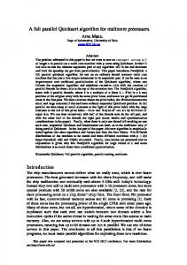
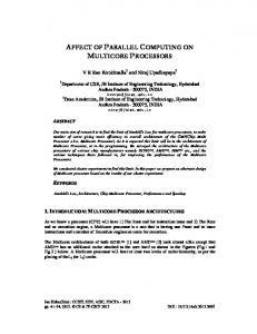
2.1 Radio astronomy Radio astronomy is a subfield of astronomy that studies celestial objects at radio frequencies. Many celestial bodies emit radio signals, and some, such as pulsars and quasars, can only be observed this way. In reality, celestial objects emit electromagnetic radiation across a wide spectrum, but only a certain range of radio frequencies can penetrate the Earth’s atmosphere sufficiently to be observed (see Figure 2.1). Of this range, LOFAR observes the lower frequencies. Figure 2.1 also shows that traditional optical astronomy only observes a very small frequency range in the spectrum, hence radio astronomy can reveal much more about the galaxy. For example, the discovery of cosmic microwave background radiation [34] was made through radio astronomy, providing evidence of the Big Bang.

Fig. 2.1: Penetration of electromagnetic radiation through Earth’s atmosphere.

2. Background

10

Any matter that is heated above absolute zero emits some electromagnetic radiation. In theory, it is possible to detect radiation from any object in the universe. Electromagnetic radiation is produced by either thermal or non-thermal mechanisms. Thermal radiation includes infrared, ultraviolet, and visible light. Non-thermal radiation includes synchrotron radiation, which is formed by particles that circle or spiral a magnetic field at velocities reaching the speed of light [18]. In radio astronomy there is a great deal of interference from natural and human-made sources. Natural sources include radio emissions from the Sun, lightning, and emissions from charged particles (ions) in the upper atmosphere. Human-made sources include power generators/transformers, radar, radio transmissions, cell phones, and GPS [18]. Radio telescopes filter this interference as best as possible, although it is never possible to remove it all. An important difference between radio and optical astronomy is that the wave characteristics of the radio signal are preserved. Incoming analog signals are converted to digital and further processed using a multitude of digital signal processing techniques. This is normally done using dedicated, custom-built hardware, which is expensive to design and maintain. In contrast, LOFAR processes signals in software, which was not possible until before the last decade when computers became fast enough to replace special hardware.

2.2 The LOFAR software telescope Radio astronomy has been traditionally conducted using radio telescopes, which consist of large dishes that can be aimed in a direction. There are two such telescopes in the Netherlands: the Dwingeloo telescope (1954 - 1990) and the Westerbork telescope (1970 - now). Over the years radio telescopes have become larger and larger to observe more frequencies and to increase the field of view (the area of the sky that can be observed). However, large telescopes are becoming too expensive to build and maintain. The LOFAR telescope is a new generation radio telescope without dishes and performs digital signal processing in software using a signal processing pipeline, allowing a great deal more flexibility and capabilities than other radio telescopes.

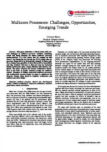
Fig. 2.2: Overview of the LOFAR signal processing pipeline.

The signal processing pipeline used by LOFAR is divided into three parts: in the field processing, real-time central processing and offline processing (see Figure 2.2). Some astronomical objects can only be observed at high sample rates, and must be studied in the real-time pipeline. The data from the real-time pipeline is also downsampled and stored, so that other, less time critical

2. Background

11

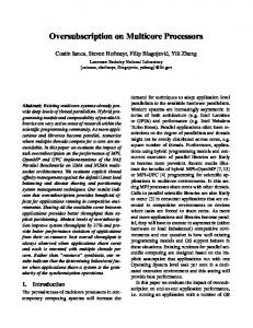
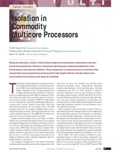
astronomical research can be conducted offline. However, LOFAR generates so much data that storage is limited to about a week’s worth of data. Radio signals are received with antennas. Antennas are grouped in stations where their samples are combined and transported to the real-time central processing pipeline. There are two kinds of antennas: low band antennas (LBA, see Figure 2.3) which detect signals in the frequency range 15-80 Mhz and high band antennas (HBA, see Figure 2.4) which detect signals in the range 110250 MHz. Antennas are polarized and take samples in orthogonal (X and Y) directions. Each station contains 48-96 LBAs and 48-96 HBAs. The signals are initially filtered using FPGAs and split into 512 subbands of 195kHz. A sample is a complex number of (2 x 4-bits), (2 x 8-bits) or (2 x 16-bits) that represents the amplitude and phase of a signal at a particular time. The samples are then sent to the central processing pipeline over dedicated fiber using UDP. LOFAR does not use TCP because it is too complicated to implement in hardware, and retransmissions would take too long in the real-time pipeline. In practice the data loss is minimal and easily tolerated [17, 36].

Fig. 2.3: Low band antenna.

Fig. 2.4: High band antenna.

2.2.1 The imaging pipeline The imaging pipeline is responsible for correlating the samples from all stations with all stations, so that an image of the observed sky can be created. See Figure 2.5 for an overview of the imaging pipeline.

Fig. 2.5: Overview of the LOFAR imaging pipeline.

2. Background

12

Correlator The function of the correlator is to filter out noise from all signals received by the antennas, leaving only the interesting signals from astronomical objects one wants to study. The received signals from sky sources are so weak, that the antennas mainly receive noise. To see if there is statistical coherence in the noise, simultaneous samples of each pair of stations are correlated by multiplying the sample of one station with the sample of the other station [36]. To reduce the output size, the products are integrated by accumulation. The integration time is approximately one second. LOFAR uses an FX correlator (F for Fourier transform and X for multiplication or correlation). The idea of an FX correlator is that the incoming signal is divided into different frequencies using a filterbank and each of those signals are then correlated with all of the signals at the same frequency among all antennas [19]. This makes it the most time consuming operation in the pipeline with a time complexity of O(n2 ) (all other pipeline stages have lower time complexity) [37, 36]. Polyphase filterbank In the LOFAR system, frequency splitting is performed by the polyphase filterbank. Each 195 KHz wide subband that comes from the stations is split into a number of consecutive frequency channels (256 is the common case). The polyphase filter itself consists of as many Finite Impulse Response (FIR) filters. Next, the filtered data is Fourier transformed yielding the same amount of frequency channels, each 763Hz wide [35, 36]. Chapter 3 explains how the polyphase filter works in more detail, and chapter 4 describes our implementation of it. Phase shift Since light travels at a finite speed, two antennas do not receive a wave at the same time (see Figure 2.6). To correlate two signals, the signal from one of the receivers must be delayed to compensate for the difference in travel time. The delay depends on the distance of the receivers and the direction in which the receivers observe. This is complicated by the rotation of the earth, which alters the orientation of the stations with respect to the observed sky continuously [35]. This is achieved by simply delaying a sample stream by an appropriate amount.

Fig. 2.6: The left antenna receives the wave later.

Bandpass correction The filterbank that runs on the FPGAs introduces artifacts that must corrected by multiplying each complex sample by a real, channel-dependent value that is computed in advance. If this correction is not done, some stations will have a stronger signal than others [36]. Beamforming This step is optional and adds the samples from a group of stations that are close together to form a virtual ”superstation” with more sensitivity. By applying an additional phase rotation (complex multiplication), beam forming can also be used to select observation directions, or to observe different parts of the sky simultaneously [36].

2. Background

13

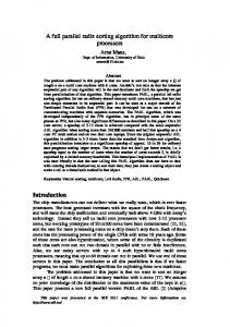
The result of the imaging pipeline is an image such as the one in Figure 2.7, which is the first image ever taken by LOFAR (the image quality has since been improved). In the remainder of this thesis, we focus on the polyphase filter and its implementation or multi-/many-core processors.

Fig. 2.7: The first image ever taken by LOFAR.

2.2.2

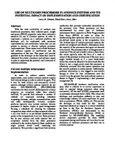
Performance on the Blue Gene/P

Figure 2.8 shows the performance of the pipeline stages on one compute node on the Blue Gene/P. The Figure shows that the polyphase filter (FIR + FFT) is the second most time consuming stage, after the correlator. The BG/P used by LOFAR contains 12480 processor cores that provide 42.4 TFLOP/s peak processing power. One chip contains four PowerPC 450 cores, clocked at 850 MHz, each of which has two Floating Point Units (FPUs). The compute nodes run a fast, simple, single-process kernel (Compute Node Kernel, CNK) [36].

2. Background

Fig. 2.8: Performance of imaging pipeline stages on one compute node of the Blue Gene/P.

14

3. SIGNAL PROCESSING

In this section we give a short introduction in signal processing, covering the basic concepts needed to understand polyphase filters and how they work.

3.1 Signals A signal is defined as any physical quantity that varies with time, space, or other independent variable(s) [32]. A signal can be mathematically described as a function of one or more independent variables. Continuous-time (analog) signals are defined for every value of time, whereas discrete signals are only defined at certain specific times. In this thesis, we are only interested in discrete signals. An example of a discrete signal is x(n) = e|n| , n ∈ N, where n describes the index of the discrete time instant. Discrete signals can either be sampled at (usually) equally spaced intervals from an analog signal source or by accumulating over a period of time. LOFAR antennas sample discrete, complexvalued samples at a fixed interval (defined by the sampling frequency). The sampling frequency of LOFAR is 160 or 200 MHz.

3.2 FIR filter A Finite Impulse Response (FIR) filter multiplies a finite number of recent input signals (impulses) relative to a given discrete time by coefficients (impulse responses) and accumulates the N ∑ results. It can be written mathematically as y(n) = ci x(n − i), where: i=0

• y(n) is the output signal at discrete time n. • x(n) is the input signal at discrete time n. • ci are the coefficients, also called weights. • N is the number of recent signals to consider, called the filter order. The terms on the right-hand side of the equation are called taps. An N-th order FIR filter has N + 1 taps. A FIR filter must remember its last N input samples, which are stored in what is called the delay line. One can design a FIR filter by carefully choosing the filter order and coefficients such that the system has specific characteristics. For the purpose of our work, those values are predetermined. A simple example of a FIR filter is the moving average, which computes the average of the most recent N + 1 input signals. In this case all coefficients have the value N1+1 . A 4-tap moving average filter can be written as: y[n] = 14 x[n] + 14 x[n − 1] + 14 x[n − 2] + 14 x[n − 3] (see Figure 3.1).

3. Signal processing

z -1

x[n]

1/4

z -1

16

z -1

1/4

1/4

1/4

+

+

+

y[n]

Fig. 3.1: Block diagram of a 4-tap moving average FIR filter. The incoming sample x[n] and the samples in the delay line z −1 are multiplied by 14 and accumulated. All samples in the delay line move to the next tap, and the incoming sample x[n] is stored in the front.

3.3 Discrete Fourier Transform A Fourier transform splits a sequence of input signals into a sequence of frequencies. In doing so it transforms the input from the time domain to the frequency domain. It can be compared to how a prism splits white light into separate light beams of a single frequency (see Figure 3.2).

Fig. 3.2: A prism splits white light into separate light beams of a single frequency.

A Discrete Fourier Transform (DFT) operates on discrete signals and can be written mathematN∑ −1 2π ically as fk = x(n)e−i N nk , where: n=0

• x(n) is an input signal; there are N input signals. • fk is the kth frequency and is a complex number, k = 0, 1, 2, ..., N − 1. The complexity of this algorithm is O(N 2 ), since computing any of the N frequencies requires iterating over N inputs. This algorithm is not used directly in practice, because there are better algorithms known as Fast Fourier Transforms (FFT) which have a complexity of only O(N log2 (N )). 3.3.1

Fast Fourier Transform

As mentioned, a FFT can compute a DFT in O(N log2 (N )) time. In this subsection we explain how this can be accomplished and further optimized using parallellization. We briefly describe the radix-2 Cooley-Tukey FFT algorithm [16], because it is a well known and easy to understand algorithm. The Cooley-Tukey algorithm, computes a DFT as two interleaved DFTs by the parity (even or oddness) of the summation index in the previously shown equation. By recursively

3. Signal processing

17

splitting the two interleaved DFTs, a time complexity of O(N log2 (N )) is achieved. Let us take a DFT with N = 8 and write out the summation [5]: fk = x(0) + x(1)e−i + x(4)e−i

2π 8 4k

+ x(2)e−i

2π 8 k

+ x(5)e−i

2π 8 5k

2π 8 2k

+ x(3)e−i

+ x(6)e−i

2π 8 6k

2π 8 3k

+ x(7)e−i

(3.1)

2π 8 7k

Then we sort the terms by parity, effectively splitting the FFT into two smaller FFTs: fk = [x(0) + x(2)e−i +e

−i 2π 8 k

2π 8 2k

+ x(4)e−i

[(x(1) + x(3)e

−i 2π 8 2k

2π 8 4k

+ x(6)e−i

+ x(5)e

−i 2π 8 4k

2π 8 6k

]

+ x(7)e−i

2π 8 6k

(3.2) )]

And split the sums again: fk = [(x(0) + x(4)e−i +e

−i 2π 8 k

2π 8 4k

) + e−i

[[(x(1) + x(5)e

−i 2π 8 4k

= [(x(0) + x(4)e−iπk ) + e

2π 8 2k

((x(2) + x(6)e−i

)+e

−i π 2k

−i 2π 8 2k

2π 8 4k

)]

((x(3) + x(7)e−i

2π 8 4k)

)]

(x(2) + x(6)e−iπk )]

(3.3)

+ e−i 4 k [(x(1) + x(5)e−iπk ) + e−i 2 k (x(3) + x(7)e−iπk )] π

π

So, there are 3 (log2 (8)) levels of summation, and each level can be parallellized by computing each summation in different threads. In this example we need 4 threads for the inner summations, 2 for the middle, and 1 for the outer summation. There are k frequencies to compute, which can all be done in parallel as well. The final observations are that ei(ϕ+2π) = eiϕ and ei(ϕ+π) = −eiϕ , meaning even and odd frequencies share the same multipliers, and can thus share much data.

3.4 Polyphase filter Polyphase filters are used by LOFAR to channelize input streams and reduce interference. A polyphase filter splits the input sequence into subsequences of M samples, where each subsequent input signal is the input to one of M FIR filters (or channels). This can be described N ∑ mathematically as ym (n) = ci x((n − i)M + m), where: i=0

• N is the number of recent samples to consider (the filter order). • M is the number of FIR filters (channels). • ym (n) is the nth output signal of the mth FIR filter, m = 0, 1, 2, ..., M − 1. The M outputs ym (n) are used as inputs to a Discrete Fourier Transform as described in the previous subsection. Figure 4.1 shows a schematic of a polyphase filter in the LOFAR pipeline, where the input stream is channelized into 256 channels, which are then fourier transformed.

4. IMPLEMENTATION

In this chapter we explain in detail how the polyphase filter is implemented on each of the following architectures: Intel Core i7 920, NVIDIA GTX480 Fermi, Microgrid, and ATI HD5870. We include description of the memory layouts of the data structures, optimization techniques and performance statistics. The implementation details that are common to all architectures will be discussed first. We sometimes use the term kernel, which refers to the functions in our application that perform the polyphase filter operations. Each implementation is designed as a library that can be included in different programs. The API1 of all libraries is as similar as possible, but there are some differences simply because the architectures have different properties. The API documentation is included separately with the thesis. We focused on the implementation of the FIR filter. We did not implement the FFT ourselves, but used a third-party library when possible. The reason for this is that implementing an optimized FFT is a very time consuming task, and there are already high performance implementations available.

4.1 Polyphase filter The LOFAR polyphase filter handles multiple stations, but they are completely independent (”embarrassingly parallel”). Therefore, in this section we explain how the polyphase filter functions for a single station. The input to the polyphase filter are samples received from the stations in the field. Samples are complex numbers of (2 x 4-bit), (2 x 8-bit) or (2 x 16-bit) integers, which are first converted to 32-bit floating point values. All computation is further done using 32-bit floating point values. The number of received samples per time unit is equal to the number of channels times the number of polarizations (two, X and Y). There is a separate FIR filter for each channel and polarization. The FIR coefficients are the same for both polarizations. There is one FFT per polarization and the outputs of the channel FIR filters, divided by polarization, form the input to them. The output of the FFTs represents the output of the polyphase filter (see Figure 4.1). A FIR filter must remember its last few input samples to compute its next output. These are stored in a delay line, which can be seen as a bounded FIFO buffer with a size equal to the number of taps. When a FIR filter gets a new input it is stored at the front of the buffer and all samples shift to the next tap (so the newest becomes the second-to-newest, etc) and the sample that was in the last tap is discarded. We cannot use strength reduction to reduce the computational complexity, because that involves designing a specific FIR filter for a specific set 1

Application Programming Interface

4. Implementation

19

Fig. 4.1: Schematic of a polyphase filter. The delay compensated input stream is channelized into 256 channels, which are then Fourier transformed.

of coefficients. But in LOFAR the coefficients are not fixed and can be changed at any time. Figure 4.2 shows high-level pseudo code of the polyphase filter algorithm. We make some observations to guide our implementation and optimizations: • All FIR filters of all channels and polarizations can be computed independently and in parallel. • Coefficients are shared between polarizations, so it may be efficient to compute both polarizations of a channel in the same kernel. • The FFTs can also be computed in parallel, but not before all FIR filters of a given polarization are computed. • The delay lines are reused for every new sample and the way in which they are stored must be considered carefully to minimize data copying. • All input and output data for the FIRs and FFTs are stored at different non-overlapping memory locations, so there is no need for any kind of locking and there are no critical sections.

4. Implementation

1 2 3

4 5 6 7 8 9 10 11 12

20

foreach Station St do foreach Polarization Po do foreach Channel Ch do /* Get the new sample, store it in tap 0 of the delay line of this station’s channel and polarization, then compute the result. */ S ← GetSample(St, Ch, Po); PutDelayLine(St, Ch, Po, S); FirSum ← 0; for Idx ← 0 to Ntaps − 1 do Tap ← GetDelayLine(St, Ch, Po, Idx); Coeff ← GetCoefficient(Ch, Idx); FirSum ← FirSum + Tap × Coeff; PutFirOutput(St, Ch, Po, FirSum); ComputeFFT(St, Po); Fig. 4.2: Polyphase filter high-level pseudo code.

4.1.1

Data structures

In this subsection we explain the memory layout of the data structures used by the polyphase filter. The memory layout is important because it has a big impact on cache efficiency and/or memory coalescing. There are four data structures: • The input array, where incoming samples from the stations are stored, one for each channel and polarization. • The output array, where polyphase filter output samples are stored. • The delay line array, where the taps of all FIR filters are stored. • The coefficients array, where the coefficients used by the FIR filters are stored, one for each channel and tap. All stations share the same coefficients. The layout of the input and output arrays is the same for all implementations, because it is given by the LOFAR imaging pipeline. The delay line and coefficients arrays are only used internally and their layout is not the same for all architectures, so we will come back to them later to explain the optimal layout. The input array is a four-dimensional array of samples where the dimensions are (in order): time, station, channel, polarization. Note that the polarizations are interleaved, as this is how the samples are received from the stations (see Figure 4.3). The output array is a four-dimensional array of samples where the dimensions are (in order): time, polarization, station, channel. The output array is divided into two parts, one for each polarization (see Figure 4.4). This array is also used as input to the FFTs, so all samples that belong to one station must be stored in consecutive memory locations (see Figure 4.3).

4. Implementation

21

The delay line array is a four-dimensional array of samples and it is only used internally. Its dimensions are: station, channel, tap, polarization. The exact order of dimensions differs per implementation due to differences in memory access patterns. A graphical representation to clarify will be given later for each architecture. The coefficients array is only used internally and it stores the coefficients used by the FIR filters. The dimensions are: channel, tap. Note that polarizations share the same coefficient per channel per tap. Just like the delay line array, the exact order of dimensions differs per implementation.

Polyphase Filter (1 station) t taps

c channels, 2c samples X0 Y0 X1 Y1 ... ... Xc Yc

2c FIR Filters

X00 Y00 X01 Y01

... ...

X0t Y0t

X10 Y10 X11 Y11

... ...

X1t Y1t

... ... ... ... ... ... ... ...

Output X0 X1 ... Xc Y0 Y1 ... Yc

Xc0 Yc0 Xc1 Yc1

Xct Yct

2c Delay Lines (interleaved)

In place transform

FFT X

... ...

c channels

Input

FFT Y

Fig. 4.3: Memory layouts and datapaths of the polyphase filter for one station. The coefficients array is not shown, but it has the same structure as the delay lines.

Input Array (interleaved) S0

XYXYXYXY...

S1

XYXYXYXY...

...

Ss

XYXYXYXY...

Polyphase filters

S0X S1X

...

SsX S0Y S1Y

...

SsY

Output Array (separated) Fig. 4.4: The polyphase filters take interleaved (by polarisation) input and give separated output. In this figure, S0 through Ss represent the stations.

4. Implementation

Array Input Output Delay line Coefficients

Dimensions time, station, channel, polarization time, polarization, station, channel station, channel, polarization, tap channel, tap

Data type Complex I4/I8/I16 Complex F32 Complex F32 Real F32

22

Internal/External External External Internal Internal

Fig. 4.5: Overview of the data structures. I4/I8/I16 means 4/8/16-bit integer and F32 means 32-bit floating point.

4.2 Measuring performance In this section we explain how we measure the performance of our kernels. 4.2.1 Floating point operations (FLOPs) Computing the output of a FIR filter requires a number of multiply-add operations. There are Ntaps complex samples in the delay line. Each sample is multiplied by a real coefficient and these results are summed. This requires 2Ntaps floating point multiplications and 2(Ntaps − 1) floating point additions. The total amount of FLOPs per FIR filter is thus 2 + 4(Ntaps − 1). Since we use third-party FFT libraries we do not know the exact number of FLOPs for the FFT, but it be can approximated as 5Nchannels log2 (Nchannels ) [25]. LOFAR only uses power of two FFTs, because those can be computed most efficiently. 4.2.2 Memory traffic Computing the output of a FIR filter requires the following memory loads and stores (after conversion of the input samples to floating point): • Read one (2 x 4 bit), (2 x 8 bit) or (2 x 16 bit) input sample, which is converted to a (2 x 32 bit) floating point sample. Note that for simplicity of the calculations we need to make we assume (2 x 16 bit) samples. • Read (Ntaps − 1) (2 x 32 bit) samples from the delay line. • Read Ntaps 32 bit coefficients. • Write one (2 x 32 bit) output. • Write one (2 x 32 bit) sample to the delay line. So, the total amount of memory traffic for one FIR filter is 4 + 8(Ntaps − 1) + 4Ntaps + 8 + 8 = (12Ntaps − 4) + 16 bytes. One FFT has in total 4Nchannels [25] complex floating point inputs and outputs, so the amount of memory traffic is 8 × 4Nchannels = 32Nchannels bytes.

4. Implementation

23

4.3 Peak performance We use the Roofline model[39] to determine the maximum attainable performance of our implementation on a given architecture: peakmax = min(perfpeak , M emoryBandwidth × AI), where: • perfmax is the maximum attainable floating point performance of our implementation on the given architecture (GFLOP/s). • perfpeak is the theoretical peak floating point performance of the architecture (GFLOP/s). • M emoryBandwidth is the peak memory bandwidth of the architecture (GB/s). • AI is the arithmetic intensity of the implementation, which is defined as the number of FLOPs per byte of memory traffic. The AI of the polyphase filter is given in the following subsection. Using the Roofline model we can determine whether our kernels are bounded by computational power of the processor or by the memory bandwidth. If the measured performance of a kernel is lower than perfmax , it is memory bound. Otherwise, it is compute bound. Note that the Roofline model does not take some optimizations, such as memory caching, into account. This means that the measured performance can be higher than perfmax . 4.3.1

Arithmetic intensity

To use the Roofline model, we must determine the arithmetic intensity of our kernel. Arithmetic intensity is defined as the number of FLOPs per byte of memory traffic, so we need to calculate both. We calculate the AI of the FIR filter and FFT separately. F LOPf ir = 2 + 4(Ntaps − 1) BytesAccessedf ir = (12Ntaps − 4) + 16 AIf ir = F LOPf ir /BytesAccessedf ir (4.1) F LOPf f t = 5Nchannels log2 (Nchannels ) BytesAccessedf f t = 32Nchannels AIf f t = F LOPf f t /BytesAccessedf f t Note that for some implementations there are optimizations which influence the AI, this is explained in the appropriate sections.

4.4 Validation A test program was written for all implementations. It has two purposes: to verify the correctness of the implementations and to take performance measurements of the various optimization techniques that will be discussed in this chapter.

4. Implementation

24

4.4.1 Correctness of the implementation The polyphase filter consists of two algorithms that can be tested separately: the FIR filter and the FFT. To verify the correctness of the FIR filter, we compute a small moving average filter with fixed input. The output is printed to the screen and easily verified. Since we use third-party FFT libraries for most architectures, we assume they function correctly. We only verify that we are using the libraries correctly. 4.4.2

Performance measurements

The test program measures performance based on a number of parameters, both general parameters and implementation-specific parameters. General parameters are given to the program at run time. Implementation-specific parameters usually need to be hard-coded. General parameters: • Sample size (4, 8 or 16 bits). • Number of stations. • Number of channels. • Number of taps. • Number of input samples per channel, or in other words the number of times to run the polyphase filter. Implementation-specific parameters include enabled optimizations (determined at compilation time) and additional command line parameters, for example the number of threads in the CPU implementation. The following metrics are used to evaluate performance: • Running time in seconds of computing the total number of samples, measured with the highest precision timer available on a given platform. • Average running time per sample, meaning the time spent for all channels of all stations to process one input sample. • Energy consumption in Watt, measured with an external device. See section 6.2.

4.5 Properties of the architectures In this section we list the hardware properties of the architectures on which we have implemented the polyphase filter. The architectures are Intel Core i7 920, NVIDIA GTX 480 Fermi, ATI Radeon HD 5870 and Microgrid. Table 4.1 shows the properties of each architecture. Note that these numbers show the theoretical peaks. Also note that the host-to-device bandwidth of the GPUs is low due to the PCI Express 2.0 bus. Note that for Microgrid we use a simulator, and the specifications apply to the specific configuration that we have chosen for our experiments. This is explained in Section 4.8.

4. Implementation

Hardware properties Cores x FPUs/core SP FP operations/cycle/FPU Clock Frequency (GHz) GFLOPs/chip Registers/core x register width L1 cache size/chip (KB) L1 cache bandwidth (GB/s) Memory bandwidth (GB/s) Host-device bandwidth (GB/s) Process technology (nm) Thermal Design Power (W) GFLOPs/W (based on TDP)

Intel Core i7 4x4 2 2.67 85 16x4 32 ? 25.6 n.a. 45 130 0.65

NVIDIA GTX 480 480x1 1 FMA 0.7 1345 1024x4 16 or 48 ? 177.4 8.0 40 250 5.38

25

ATI HD 5870 320x5 1 FMA 0.85 2720 1024x4 8 1088 154 8.0 40 188 14.47

Micro Grid 64x1 1 1.0 64 1024x8 1 1 ? n.a. n.a. n.a. n.a.

Tab. 4.1: The hardware properties of each architecture we have investigated. FMA means Fused Multiply-Add, a single instruction that performs a multiplication and an addition. Note that the Microgrid properties only apply to the specific configuration we have chosen.

4.6 Intel Core i7 920 In this section we discuss our implementation of the polyphase filter on the Intel Core i7. We implement the FIR filter ourselves, but we use the popular FFTW library [6] to compute the FFTs. The programming language is C using the C99 standard and the compiler is gcc version 4.4.1 (Ubuntu 4.4.1-4ubuntu9). Compiler flags: -msse4 -std=gnu99 -fopenmp -O1 -s -fomit-frame-pointer -fstrict-aliasing In this implementation we compute the FIR output of both polarizations of a channel at the same time. There are three reasons for this: • The samples are adjacent to each other in memory, so this increases cache efficiency. • They both share the same coefficients, so these can be reused. • The samples consist of 4 32-bit floating point values, which fit exactly in one 128-bit SSE register. More on this optimization is explained later in section 4.6.2. In the delay line array the taps for both polarizations of a channel are also stored interleaved. The dimensions of the delay line array are as follows (in order): station, channel, tap, polarization. This way the memory here is also accessed sequentially, which increases cache efficiency (see Figure 4.3). To compute the FIR output we need to iterate over all taps in the delay line from newest to oldest. The simplest way would be to always iterate from index 0 to Ntaps − 1, but then we would need to copy the samples to shift them to the next tap each time the FIR gets a new input. We can avoid all this unnecessary copying by turning the delay line array into a bounded FIFO buffer. A delay index counter is kept, which represents the starting index of the array and also the index where the next input sample is stored. Its initial value is zero. The counter

4. Implementation

26

is decremented before the store and can have values in the range {0, 1, ..., Ntaps − 1}. This also overwrites the oldest sample, which has to be discarded anyway. Since all channels of all stations are computed in lock-step, we can share the delay index between all channels. Figure 4.6 shows pseudo code of the reference algorithm2 . In the following subsections we discuss more complex optimizations we have implemented for this version of the polyphase filter.

1 2 3 4 5 6 7

8 9 10

11

12 13 14 15

16 17 18 19 20 21

// This will decrement and ensure DelayIndex ∈ {0, 1, ..., Ntaps − 1}. DelayIndex ← (Ntaps + DelayIndex - 1) mod Ntaps ; foreach Station St do foreach Channel Ch in St do NewSampleX ← GetInputSampleX(Ch) // X and Y polarizations. NewSampleY ← GetInputSampleY(Ch); PutDelayLineX(Ch, DelayIndex, NewSampleX); PutDelayLineY(Ch, DelayIndex, NewSampleY); // 2 * 2 FLOPs (samples are complex) SumX ← NewSampleX * GetCoefficient(Ch, 0); SumY ← NewSampleY * GetCoefficient(Ch, 0); CoIdx ← 1; // Coefficient index. // Both loops together make Ntaps − 1 iterations. for Idx ← DelayIndex + 1 to Ntaps − 1 do // 2 * 4 FLOPs SumX ← SumX + GetDelayLineX(Ch, Idx) * GetCoefficient(Ch, CoIdx); SumY ← SumY + GetDelayLineY(Ch, Idx) * GetCoefficient(Ch, CoIdx); CoIdx ← CoIdx + 1; for Idx ← 0 to DelayIndex − 1 do // 2 * 4 FLOPs SumX ← SumX + GetDelayLineX(Ch, Idx) * GetCoefficient(Ch, CoIdx); SumY ← SumY + GetDelayLineY(Ch, Idx) * GetCoefficient(Ch, CoIdx); CoIdx ← CoIdx + 1; PutOutputX(Ch, SumX); PutOutputY(Ch, SumY); ComputeFFTs(); Fig. 4.6: CPU reference implementation.

4.6.1

Multi-threading with OpenMP

The polyphase filter is trivially parallelizable, since all channels of all stations are independent and only share constant data. We use OpenMP [10] to parallelize the outer loop shown in Figure 4.6, so that each thread computes a number of stations. This required only a single pragma: #pragma omp parallel for if(nr stations >= 2) Since the polyphase filter computes two filters in sequence, but individual stations are independent, we can interleave the FIR and FFT computations in the same thread. This way we need 2 Although what we have discussed so far technically includes optimizations, we believe they are straightforward and do not significantly increase code complexity, if at all.

4. Implementation

27

less thread synchronization, improving efficiency. Moreover, a portion of the output array may still be in the cache, increasing cache hits. Figure 4.7 shows the effect of varying the number of threads on the performance on the Intel Core i7. We only show one example (16 stations x 256 channels x 16 taps x 16-bit samples), because experiments with different parameters show the same behaviour. Although the Core i7 has hyperthreading, the optimal number of threads is four, equal to the number of cores. 4.6.2

Vectorization with SSE

The first optimization we implemented was to use Intel’s SSE3 instruction set [22]. SSE is an instruction set extension that makes a number of SIMD4 instructions and registers available to the CPU. The registers are 128-bit and can hold four 32-bit floating point values in subregisters. SSE instructions operate on each subregister simultaneously. The compiler does not generate SSE code by itself, SSE enabled code must be written explicitly by the programmer. We don’t need to write assembly, because access to the registers and instructions is provided via compiler intrinsics. The compiler does take care of register allocation. SSE registers can only be loaded/stored efficiently if the source/destination memory addresses are aligned on a 16-byte boundary. We use memory allocation functions from the FFTW library to ensure all our arrays are aligned on this boundary. Even so, some values (such as the 4 and 8-bit samples) are too small to always be aligned on this boundary. In this case we have to load the SSE registers from intermediate general registers instead. We use three SSE registers: • One to store the sums (see Figure 4.6). • One to store two samples read from the delay lines. • One to store the coefficient. SSE has a total of 16 registers (XMM0 through XMM15), which is enough to store an entire delay line, but that would not leave any room for the other registers we need. The 8 and 16-bit input samples are loaded and converted to floating point in one SSE instruction, which also conveniently places them in the SSE register we use to store the sums. The 4-bit samples must first be loaded into an MMX5 register, and are converted to floating point from there. The samples from the delay lines are loaded in one instruction, note that this would not be possible if the polarizations in the delay lines were not interleaved. Coefficients are single floating point values, which we replicate in all four subregisters using the mm set1 ps intrinsic. Figure 4.8 compares the performance of using different sample sizes for the reference and optimized implementations. In the reference implementation there is almost no difference between sample sizes. Interestingly, in the optimized implementation 8-bit samples are more efficient than 16-bit samples. We believe this is because, while (2x 8-bit) and (2x 16-bit) samples are both loaded in one SSE instruction, (2 x 8-bit) samples require only half the amount of memory. 3 4 5

Streaming SIMD Extensions Single Instruction Multiple Data MultiMedia Extensions, SIMD instructions for integers only.

4. Implementation

28

Fig. 4.7: The impact on performance of varying the number of threads on the overall performance of the optimized implementation on the Intel Core i7. We show the performance of the FIR filter in isolation (left) and that of the complete polyphase filter (right).

4. Implementation

29

To compute we simply multiply all four sample values by the coefficient and then add the result to the sums. The available SSE instruction sets (SSE1 through SSE4) do not include a fused multiply-accumulate instruction, so we use the two intrinsics mm mul ps and mm add ps. However, SSE5, which is in development at the time of writing, will include a fused multiplyaccumulate instruction [14] that performs both computations at once. We note that by using SSE instructions, we obtain a performance increase of approximately 1.6x compared to the reference implementation (see Figure 4.7). 4.6.3 Loop unrolling Loop unrolling is an optimization in which the body of a loop is performed multiple times in one iteration, thereby reducing the total number of jumps required to complete the loop, at the expense of increased code size. The compiler can sometimes perform this optimization automatically. In our case this is not possible, because the number of loop iterations cannot be determined statically, and is always a different number (see Figure 4.6). We unrolled the loop once and dealt with an uneven number of total iterations (taps) separately, as seen in Figure 4.9. Partially unrolling the loop has the advantage of being able to use almost any number of taps. Whereas if the loop were unrolled completely, we would need separate functions for different numbers of taps, and that would mean the possible numbers of taps is hardcoded. In addition, loop unrolling increases code size which means it might not fit completely into the instruction cache, and that has a negative impact on performance. 4.6.4 Maximum performance To compute the maximum performance, we need to know the number of flops and bytes accessed per FIR filter and FFT. For the FIR reference implementation and FFT we already know the number of flops and bytes accessed from section 4.3. Since we use SSE to compute two polarizations at once, the numbers are computed differently for the optimized implementation: F LOPf ir,ref = 2 + 4(Ntaps − 1) BytesAccessedf ir,ref = (12Ntaps − 4) + 16 F LOPf ir,opt = 4 + 8(Ntaps − 1) BytesAccessedf ir,opt = (20Ntaps − 8) + 32

(4.2)

Based on these equations, we can compute the arithmetic intensity and peak performance of the polyphase filter. From Table 4.1 we know that perfpeak = 85 GFLOP/s and M emoryBandwidth = 25.6 GB/s. The performance of the FIR depends on Ntaps , and the performance on the FFT depends on Nchannels . The peakmax in GFLOP/s for the FIR and FFT are shown in Table 4.2. The observed performance is actually much higher, due to the effect of caching.

4. Implementation

30

Fig. 4.8: Performance of processing 4/8/16-bit samples on the Intel Core i7 for the reference and optimized implementations. We show only the performance of the FIR filter, because the FFT is not affected by the input sample size. Reference on the left, optimized on the right. The optimized implementation includes SSE and loop unrolling.

4. Implementation

1 2 3 4 5 6 7 8

9 10 11 12 13 14 15

31

/* After computing the first odd tap there can only be a multiple of two taps left since we know Ntaps is always even. */ Idx ← DelayIndex + 1; if Idx is odd then ComputeTap(); Idx ← Idx + 1; while Idx < Ntaps do ComputeTap(); ComputeTap(); Idx ← Idx + 2; /* Compute all even pairs, if the last tap is odd then compute it separately. Idx ← 0; while Idx < DelayIndex − (DelayIndex mod 2) do ComputeTap(); ComputeTap(); Idx ← Idx + 2;

*/

if DelayIndex is odd then ComputeTap(); Fig. 4.9: CPU FIR loop unrolling.

Ntaps AIf ir,ref AIf ir,opt perfmax,f ir,ref (GFLOP/s) perfmax,f ir,opt (GFLOP/s) Nchannels AIf f t perfmax,f f t (GFLOP/s)

4 0.23 0.26 6.0 6.9 64 0.94 24

8 0.28 0.33 7.1 8.3 128 1.1 28

16 0.30 0.36 7.8 9.2 256 1.25 32

32 0.31 0.38 8.1 9.7 512 1.4 36

64 0.33 0.39 8.3 10.0 1024 1.6 40

Tab. 4.2: The arithmetic intensity and maximum performance of the polyphase filter on the Intel Core i7 920, determined with bound-and-bottleneck analysis (see Section 4.3). From Table 4.1 we know that perfpeak is 85 GFLOP/s and M emoryBandwidth is 25.6 GB/s.

4.6.5

OpenCL

We have compiled the vectorized OpenCL implementation, described in section 4.9, for the CPU. We chose the vectorized implementation, because it can take better advantage of SSE instructions than the non-vectorized OpenCL implementation. We were unable to run the OpenCL FFT library on the CPU, so we only present the performance of the FIR filter, seen in Figure 4.10. We can directly compare the performance of the 16 taps x 16-bit samples FIR filter in Figure 4.10 with Figure 4.7. The performance of the OpenCL implementation reaches at best approximately 10.5 GFLOP/s, while our optimized implementation reaches slightly more than 16 GFLOP/s. Again we see that 8-bits is the most efficient sample size, as previously explained

4. Implementation

32

in section 4.6.2. The reason why the OpenCL implementation performs worse may be that it uses batching (described in section 4.7.4), which is meant to exploit the architecture of GPUs. Batching completely unrolls the inner loop, meaning there are no branches, but it also increases the machine code size proportional to the number of taps. This means the machine code of the inner loop may not always fit in the CPU’s instruction cache, requiring more memory access, which impacts performance. It also requires many registers, which are available on GPUs, but not on the Core i7. This means registers must be spilled very often, decreasing performance. This shows that, although OpenCL is cross-platform, that does not mean that the same OpenCL kernel runs efficiently on all platforms. We expect that an OpenCL implementation optimized specifically for the Core i7 will achieve much better performance. 4.6.6

Discussion

This is the platform we started with. Since we were already familiar with C and OpenMP, the implementation was straightforward to write. We had not used SSE before, but it was farily straightforward to use. We had no real problems or issues with this platform. Our hand optimized implementation achieves 18.8% peak performance, while the OpenCL implementation achieves 12.4% peak performance, for 16 taps. So, our hand optimized implementation is almost 50% more efficient, similarly for other number of taps. Our hand optimized implementation achieves higher than the theoretical maximum performance, so we have good results.

4. Implementation

33

Fig. 4.10: The performance of the vectorized OpenCL implementation (described in section 4.9) of the FIR filter on the Core i7 920. We show the impact of varying Ntaps (left) and the sample size (right).

4. Implementation

34

4.7 NVIDIA GTX 480 Fermi This implementation measures performance on NVIDIA’s Fermi architecture on a GTX 480 graphics card. We implemented the polyphase filter using NVIDIA’s proprietary parallel computing programming model called CUDA6 [26]. The programming language is C with the nvcc compiler included with CUDA Toolkit 3.1. We use the CUFFT library [28] for the FFT. Compiler flags: -std=gnu99 -m64 -arch sm 20 -O1 -s -fomit-frame-pointer 4.7.1

CUDA Architecture

This section explains briefly the details most important to know about the CUDA and Fermi architecture for our implementation. CUDA is the hardware and software architecture that enables NVIDIA GPUs to execute programs written in C, C++ and other languages. A CUDA program calls parallel kernels. A kernel executes in parallel across a set of parallel threads. Threads are organized in thread blocks and grids of thread blocks [29]. Threads are executed by a Streaming Multiprocessor in groups of 32 threads called warps. Each thread starts at the same program address, but has a separate program counter, set of registers, inputs and outputs and a per thread block unique ID. If during warp execution a branching instruction in encountered, the sets of threads following each branching path are executed serially, pausing the other threads in the warp, until all paths converge. Therefore it is important, for performance reasons, to minimize diverging branches. Our implementation has no diverging branches. The CUDA architecture has four different memory spaces: global memory, constant memory, texture memory and shared memory, but we only use the global and constant memory. The global memory is the DRAM of the GPU, which is cached on the Fermi [29], but not on older architectures. The constant memory can only be written by the CPU and is accessed almost as fast as registers. The input, output and delay line arrays are kept in global memory (we will optimize this later, see section 4.7.4) and the FIR coefficients in constant memory. The delay lines cannot be stored in shared memory, because it is too small. When threads in a warp access consecutive memory locations without gaps, they are coalesced in one memory transaction, greatly increasing performance. Therefore it is important, for performance reasons, to design data structures such that accesses to it are coalesced as often as possible. Only accesses within the same warp are coalesced (see Figure 4.11). Fermi can execute 512 single-precision floating point fused multiply-add instructions per clock. 4.7.1.1

Grid and thread block layout

Threads are organized in threads blocks and grids of thread blocks (called grid blocks), which can be at most three and two dimensional, respectively. A thread block can have at most 1024 threads on the Fermi and 512 otherwise. The size of a thread block influences the occupancy of the Streaming Multiprocessor, which is an important metric for the overall utilization of the GPU (explained in more detail in section 4.7.4). 6

Compute Unified Device Architecture

4. Implementation traditional multi-core optimal memory access pattern

t=1

thread 3

t=0 t=1

address 2 address 3

thread 2

address 4 address 5

t= t=

thread 3

address 6

address 1

0

address 2

1

thread 2

t=0

= thread 1 t

t=

t=1

address 1

1

thread 1

t=0

address 0

t=

t=1

t=0

thread 0

address 0

0

1

t=

address 3 address 4 address 5

0

t=0

many-core GPU optimal memory access pattern

t=

thread 0

35

1

address 7

address 6 address 7

Fig. 4.11: Optimal memory access patterns on traditional multi-cores (left) and many-core GPUs (right). The access pattern on the right is coalesced on GPUs, because at a given time instant all memory accesses are to adjacent addresses.

For the FIR filter we choose the size of the thread block such that we achieve the highest occupancy. The thread blocks are organized in a two dimensional grid where the stations are on the X dimension. If a station requires more threads than fit in one thread block, then the threads are evenly divided into two or more thread blocks in the Y dimension. See Figure 4.12 for a graphical overview of the grid and thread blocks. All threads have a unique ID determined by the grid and thread block they are located in, and that is used to index the arrays used by the FIR filter. The parity of the thread ID determines the polarity of the samples processed by the given thread. As explained in section 4.7.6.1, the maximum threads per block is determined by the number of taps, and usually we need more than one thread block per station to compute all channels.

Thread Block

0,X 1,Y 2,X 3,Y

... ...

r-1,X r,Y

r threads per block

...

Ss0

Grid S01 S11 ... Ss1 Block ... ... ... ... S0b S1b

...

Ssb

b blocks per station

S00 S10

}

br=2Nchannels sbr total threads/ FIR filters

s stations

Fig. 4.12: Grid and threads block for the FIR filters on CUDA. The exact values for b and r are determined by the number of taps and channels. This is explained in section 4.7.6.1.

4. Implementation

36

4.7.2 Memory layout The layout of the input, output, delay line and coefficient arrays must be such that accesses to them are coalesced as often as possible. Warps always execute threads in the order of their thread ID within a thread block (see section 4.7.1.1). This means we don’t need to change the layout of the input and output arrays, because accesses to it are already coalesced. The layouts of the delay line and coefficient arrays are transposed compared to those of the CPU implementation to improve coalescing (see Figure 4.13).

GPU Polyphase Filter (1 station) c channels

c channels, 2c samples

Input

X0 Y0 X1 Y1 ... ... Xc Yc

Output X0 X1 ... Xc Y0 Y1 ... Yc In place transform

FFT X

FFT Y

... ...

Xc0 Yc0

X01 Y01 X11 Y11

... ...

Xc1 Yc1

... ... ... ... ... ... ... ... X0t Y0t X1t Y1t

... ...

t taps

2c FIR Filters

X00 Y00 X10 Y10

Xct Yct

2c Delay Lines (interleaved, transposed)

Fig. 4.13: Memory layouts and datapaths of the polyphase filter for one station on a GPU. For multiple stations the structure is simply repeated. The coefficients array is not shown, but it has the same structure as the delay lines. The only difference with Figure 4.3 is that the delay lines and coefficients array are transposed.

4.7.3 Reference implementation The reference implementation is very similar to the one we implemented on the CPU, except that each thread computes one FIR filter of one polarization. So, for each station there are 2Nchannels threads, divided over one or more thread blocks. The FFT is executed after all FIR filters are computed. The input and output arrays are buffered in host memory. The input data is copied synchronously to the device buffer before calling the kernel. The FIR kernel reads one sample and the delay line from global memory, then computes the output and writes it and the updated delay line to global memory. The FFT then does an in-place transform, after which the output array is copied back to the host memory. The FIR coefficients are kept in the constant memory, which has a much lower latency than global memory but can only be read by the GPU threads and written by the CPU. The GTX 480 has 64K bytes constant memory, which limits the maximum number of channels and taps to Nchannels × Ntaps ≤ 16384, since one coefficient is 32-bits. We need to convert the integer input samples to floating point, which is done using the int2f loat intrinsic function [26]. We found it to have an overhead of approximately 1%.

4. Implementation

37

4.7.4 Sample batch processing In the reference implementation the kernel processes one sample and exits. This requires the delay line to be loaded and stored from global memory on each call. We can keep the delay line in registers for multiple samples by changing the kernel to process batches of samples at a time. This way, the delay line is first loaded into registers, then used to process all samples in the batch, and in the end written back to global memory. Thus, the delay line is only loaded and written once regardless of how many samples are processed. Afterwards the FFT is executed for all output arrays. This kind of threading with many registers is called heavyweight threading, and is advocated by GPU programming guru Vasily Volkov [38]. As will be shown, batch processing has a big effect on the efficiency of the FIR filter. The delay line is loaded into registers by declaring each tap as a separate variable (not an array, they cannot be stored in registers). Note that this requires multiple kernels, one for each combination of input sample type and number of taps. Another drawback is that all samples to be processed must already be in memory, this requires a large amount of memory to be preallocated. This is okay because LOFAR already processes many samples at once (768 samples, or about one second of data). As explained previously, the delay line is implemented as a bounded FIFO buffer. Naively, this would require copying the contents from one tap register to the next. This can be avoided by renaming the registers manually in the code, but it means we must unroll the inner loop completely Ntaps times. This is better explained with an example, see Listing 4.14. 4.7.4.1 Maximum performance The number of samples in one batch is equal to the number of taps, this simplifies programming and allows the kernel to process multiple batches in a loop. The number of samples processed by the kernel is Nsamples = Nbatches × Ntaps . Note that the delay line is only read from and written to global memory once every Nsamples samples. Thus the number of bytes accessed is: 8N

taps BytesAccessedf ir = 2 Nsamples + 4Ntaps + 12 =

16 Nbatches

+ 4Ntaps + 12

16 Now it is clear that, as Nbatches increases, the factor Nbatches approaches zero, and effectively BytesAccessedf ir ≈ 4Ntaps +12, meaning batching effectively masks the memory access latencies that would otherwise be caused by reading/writing the delay lines from global memory. Table 4.3 shows the number of bytes accessed depending on Ntaps . Note that we assume 16-bit samples.

Since fewer memory accesses are required for the same amount of computation, the arithmetic intensity increases as Nbatches increases (see Table 4.4). Using the arithmetic intensity from Table 4.4 and hardware properties from Table 4.1 we can compute maximum performance for this platform, as shown in Table 4.5. The actual observed performance is much higher, as shown in Figures 4.16 and 4.18. We believe this is caused by the caching of the input and output arrays, as well the bandwidth of the constant memory (where we store the weights), which is much higher than that of global memory. Finally, Figure 4.17 shows the impact on performance by varying the sample size. It shows that without I/O transfers, the sample size has a small effect on performance as the batch size increases. If we include I/O transfers, 4-bit samples are by far most efficient, approximately 30% more efficient than 16-bit samples in the best case. This is because we only need to transfer 14 th as much memory compared to 16-bit samples.

4. Implementation

1 2 3 4

5 6 7 8 9 10 11 12

13 14 15

38

Input: Nbatches , the number of batches to process. /* The delay line taps are stored in variables T0 ...T3 , which are allocated to registers. First the delay line stored is copied from global memory to these variables, except for the last tap because it will be discarded when the first sample is read. */ T1 ← GetDelayLine(0); T2 ← GetDelayLine(1); T3 ← GetDelayLine(2); for BatchNum ← 1 to Nbatches do // C0 ...C1 are the FIR coefficients. T0 ← GetInputSample(); PutOutput(T0 C0 + T1 C1 + T2 C2 + T3 C3 ); T3 ← GetInputSample(); PutOutput(T3 C0 + T0 C1 + T1 C2 + T2 C3 ); T2 ← GetInputSample(); PutOutput(T2 C0 + T3 C1 + T0 C2 + T1 C3 ); T1 ← GetInputSample(); PutOutput(T1 C0 + T2 C1 + T3 C2 + T0 C3 ); /* After processing all samples the delay line is written back to global memory. The last tap does not have to be written because it will be discarded anyway. */ PutDelayLine(0, T0 ); PutDelayLine(1, T1 ); PutDelayLine(2, T2 ); Fig. 4.14: CUDA batch processing example for a 4-tap FIR filter. The code pattern is the same for FIR filters with more taps.

4. Implementation

Ntaps 4 8 16 32 64

reference (1 sample) 60 108 204 396 780

1 batch 44 60 92 156 284

2 batches 36 52 84 148 276

4 batches 32 48 80 144 272

39

8 batches 30 46 78 142 270

16 batches 29 45 77 141 269

32 batches 28.5 44.5 76.5 140.5 268.5

% of ref 48% 41% 38% 36% 35%

Tab. 4.3: The number of bytes accessed by the FIR filter on CUDA depending on the number of taps and batch size. The second column shows how many bytes are accessed when processing a single sample per kernel execution (reference implementation). The last column shows how many bytes are accessed in the best case compared to the reference implementation.

Ntaps 4 8 16 32 64

reference (1 sample) 0.23 0.28 0.30 0.31 0.33

1 batch 0.32 0.50 0.67 0.81 0.89

2 batches 0.39 0.58 0.74 0.85 0.92

4 batches 0.44 0.63 0.78 0.88 0.93

8 batches 0.47 0.65 0.79 0.89 0.94

16 batches 0.48 0.67 0.81 0.89 0.94

32 batches 0.49 0.67 0.81 0.90 0.95

Tab. 4.4: The arithmetic intensity of the FIR filter on CUDA depending on the number of taps and batches. The second column shows the arithmetic intensity of the reference implementation.

Ntaps x 32 batches perfmax,f ir,ref (GFLOP/s) perfmax,f ir,opt (GFLOP/s) Nchannels AIf f t perfmax,f f t (GFLOP/s)

4 39.0 87.1 64 0.94 166.3

8 47.9 119.6 128 1.1 194

16 53.2 143.8 256 1.25 221.8

32 56.8 159.1 512 1.4 249.5

64 56.8 167.8 1024 1.6 277

Tab. 4.5: The maximum performance of the polyphase filter on the NVIDIA GTX 480, excluding host-to-device memory transfers, determined with bound-and-bottleneck analysis (see Section 4.3). From Table 4.1 we know that perfpeak = 1345 GFLOP/s and M emoryBandwidth = 177.4 GB/s. We used the best case arithmetic intensity from Table 4.4.

4. Implementation

4.7.5

40

Page-locked host memory

CUDA supports streams to hide I/O latency by overlapping I/O transfers and kernel executions. Streams must be programmed manually. In practice reaching maximum efficiency using streams can become very complex, with many overlapping streams. CUDA provides an alternative called page-locked, or pinned host memory. Page-locked host memory can be mapped into device memory and can be allocated as write-combining, these are explained below. On a normal CUDA host-to-device memory transfer, the memory is first copied to a non-pageable buffer, then that buffer is transferred to the device using DMA. Page-locked host memory is allocated as its own non-pageable buffer, so no copying is needed. The drawback is that page-locked memory is allocated outside the operating system’s pages, reducing the amount of physical memory available for programs. Therefore allocating a large amount of page-locked memory can reduce system performance. This is not a big problem for our application, because all required memory is allocated once beforehand, and it is the only running program that uses a significant amount of memory. Mapping host memory into device memory By storing the input array in host memory, and mapping it into device memory, the same memory is addressable from both the CPU and GPU. This means we only need one buffer (in the host memory). Data transfers from the host to the device are performed implicitly by the kernel as required, performing the same job as streams [26]. Note that every memory access could potentially cause an expensive host-to-device memory transfer, if that memory is not cached on the device. Since the input array is accessed completely linearly and each element is read exactly once, there is exactly one host-to-device memory transfer for each chunk of page-locked memory that fits into the device cache. Write-combining Page-locked memory is normally allocated as cachable, but this can be disabled by allocating as write-combining. Write-combining memory frees up L1 and L2 cache resources and is not snooped during transfers across the PCIe bus, which can improve performance by up to 40%. Reading write-combining memory from the host is prohibitively slow, so it should only be used by memory that the host writes to [26]. Given the promising performance of page-locked memory we have used it to improve the performance of the polyphase filter. Thus, we allocate the input array as page-locked, write-combining and map it into the device memory. The output array is not page-locked, because the polyphase filter is normally the first stage in a pipeline and subsequent stages would further modify it. The performance gains are shown in Figures 4.15 and 4.16. The figures show that using pagelocked memory gives a significant performance boost. But perhaps more importantly, the figures also show the impact of I/O on the performance of the FIR filter and polyphase filter. Depending on the number of taps and channels, the performance can be reduced to a mere 10% compared to the non-I/O performance.

4. Implementation

41

Fig. 4.15: The execution time per sample of the optimized CUDA implementation compared to the reference implementation. The FIR filter is on the left, and the compete polyphase filter is on the right. The leftmost data point shows the performance of the reference implementation and subsequent data points show the performance of batching. The running time of 64 taps is not shown, because it is significantly higher and would make the graphs unreadable.

4. Implementation

42

Fig. 4.16: The throughput (GFLOP/s) of optimized CUDA implementation compared to the reference implementation. The FIR filter is on the left, and the complete polyphase filter is on the right. The leftmost data point shows the performance of the reference implementation and subsequent data points show the performance of batching.

4. Implementation

43

Fig. 4.17: The impact on execution time per sample (left), and performance (right) by varying the sample size on the GTX 480. We only show the FIR filter, because the sample size has no impact on the FFT.

4. Implementation

44

4.7.6 Occupancy Each multiprocessor of the GPU has a set of N registers which are allocated among the thread blocks executing on the multiprocessor. The maximum amount of threads that can be executed in parallel is thus bounded by the amount of registers per thread. This is referred to as the multiprocessor occupancy. The multiprocessor occupancy is defined as the ratio of active warps to the maximum number of warps supported on a multiprocessor of the GPU [27]. Ideally the occupancy should be 100% (meaning the multiprocessor is used optimally), but this is not always possible. We calculated the occupancy using the CUDA Occupancy Calculator [27], which calculates the occupancy based on the amount of registers per thread, the number of threads per thread block and the amount of shared memory per thread (although we don’t use shared memory). All registers are 32-bit. The amount of registers per thread depends on the number of taps. We need 2Ntaps registers for the delay line, since each sample is a 32-bit floating point complex number, and about 10 registers for other calculations. So we require 2Ntaps + 10 registers per thread. The amount of threads per block can be chosen freely as long as the bounds described above are not crossed. We chose a different number of threads per block depending on the number of taps to get the highest occupancy. Table 4.6 shows the occupancy and related numbers for compute ability 2.0 GPUs, such as the GTX 480. The GTX 480 has 32768 registers per thread block and each thread can use up to 63 registers without register spilling. Register spilling decreases performance, because excess registers are temporarily stored (spilled ) to device memory. Figure 4.18 shows how efficient different combinations of channels and taps are for optimal hardware utilization. The results show that using 16 taps is most efficient in all cases. This is because using more taps requires register spilling, and using fewer taps means the hardware is used suboptimally. Figure 4.18 also shows that for very small FIR filters (such as 16 stations x 16 channels) the performance is lower than expected. This is because the hardware simply doesn’t have enough work to do. Increasing the number of stations or channels brings the performance back to the expected level. 4.7.6.1

Threads per block

As shown in Table 4.6, the maximum size of a thread block depends on the number of taps. There is one thread for each channel and polarization in a station, so if 2Nchannels > M axT hreadsP erBlock, we must use multiple thread blocks per station. M axT hreadsP erBlock is given in Table 4.6. However, all thread blocks must have the same size, so we choose T hreadsP erBlock and BlocksP erStation such that: 2Nchannels = T hreadsP erBlock × BlocksP erStation where T hreadsP erBlock ≤ M axT hreadsP erBlock Our implementation computes T hreadsP erBlock and BlocksP erStation automatically, based on the number of channels and taps. This is also illustrated in Figure 4.12. The consequence of this dynamic sizing is that depending on the number of channels, thread blocks may be smaller than optimal, affecting performance (since the occupancy will be lower than shown in Table 4.6). We strongly recommend choosing Nchannels such that T hreadsP erBlock = M axT hreadsP erBlock.

4. Implementation

Ntaps 4 8 16 32 64

Registers per thread 18 26 42 74 138

Max. threads per block 512 512 256 128 32

Active thread blocks 3 2 3 3 7

45

Active threads 1538 1024 768 384 224

Active warps 48 32 24 12 7

Total nr. of registers 27684 26624 32256 28416 30912

Occupancy 100% 67% 50% 25% 15%

Tab. 4.6: CUDA occupancy on compute ability 2.0. Registers per thread = 2Ntaps + 10. Threads can use up 63 registers without spilling. The GTX480 has 32768 registers in total, so a 16 taps FIR filter makes near optimal use of the available registers.

Fig. 4.18: Performance graph showing the impact of the number of channels - number of taps combinations on the optimized FIR filter. The peaks are at 16 taps, showing that the most efficient hardware utilization is achieved by using 16 taps. The sample size is 16-bits.

4. Implementation

46

Fig. 4.19: The performance of the FIR filter implemented on OpenCL versus CUDA on the GTX480.

4.7.7

OpenCL

We translated the CUDA implementation to OpenCL [9], which is very easy because it was almost a one-to-one keyword replace. OpenCL requires the programmer to write more setup code (such as loading and compiling the kernel source code, and passing arguments to the kernel) than CUDA, since it does not use any C language extensions. We used Apple’s OpenCL FFT library [3], as we cannot use CUFFT. We found it to be fairly good performing, although not nearly as good as CUFFT. Figure 4.19 compares the performance of the FIR filter in OpenCL versus CUDA. Figures 4.20 and 4.21 show the impact of batching.

4. Implementation

47

Fig. 4.20: The execution time per sample of the optimized OpenCL implementation compared to the reference implementation on the GTX480. The FIR filter is on the left, and the compete polyphase filter is on the right. The leftmost data point shows the performance of the reference implementation and subsequent data points show the performance of batching. The running time of 64 taps is not shown, because it is significantly higher and would make the graphs unreadable.

4. Implementation

48

Fig. 4.21: The throughput (GFLOP/s) of optimized OpenCL implementation compared to the reference implementation on the GTX480. The FIR filter is on the left, and the complete polyphase filter is on the right. The leftmost data point shows the performance of the reference implementation and subsequent data points show the performance of batching.

4. Implementation

4.7.8

49

Discussion

Although programming for the CUDA platform is not that difficult, writing an optimized kernel is. This is because it requires a lot of prior knowledge about the underlying hardware. It is easy to make a mistake which causes a large performance drop, and it may be difficult to find out what is happening. Fortunately, the FIR filter is a straightforward algorithm and we already knew how it should work from our C implementation. The documentation on the CUDA platform is good, and there is also good tool support. The CUDA Occupancy Calculator in particular was very useful in determining optimal parameters for our kernels, and it saved a lot time testing and tuning.

4.8 Microgrid Microgrid is an NWO funded research project conducted at the University of Amsterdam, aiming to improve the speedup, programmability, power dissipation, scalability and concurrency management of many-core processor architectures [8]. It introduces a new concurrency model called Self-adaptive Virtual Processor (SVP) (see section 4.8.1). We use the Microgrid simulator to run our experiments. The simulator is cycle-accurate, meaning every detail of the architecture is simulated precisely, allowing for accurate measuring. The simulator can simulate different architectures with different memory models. We ran our experiments only on the 128-core Random Banked Memory architecture (rbm128), of which we used one place (see section 4.8.1) of 64 cores. Each core is clocked at 1 GHz. We also tried to run our experiments on some of the available architectures using COMA7 , but no matter what we tried the program either deadlocked or caused a write to invalid memory (through no fault of our own). This bug has since been fixed, but unfortunately too late for our thesis. Since the simulator is rather slow, we could not run as many experiments as on the other platforms presented in this thesis. We used version 3.2 of the Microgrid toolset. It includes a compiler for the SL programming language. SL is based on C with special extensions for Microgrid. The compiled programs run on the simulator. Compiler flags: -b mta n -O1 -s The following sections explain the SVP model, describe our reference and optimized implementations of the polyphase filter, and show the performance of those implementations. 4.8.1

SVP Model

The SVP model is a programming model based on the concurrent and hierarchical composition of homogeneous families of blocking threads. The SVP model defines all concurrency and communication in abstract terms and all mapping and scheduling of the threads is transparant to the programmer [24]. SVP is implemented as an extension of an instruction set architecture (ISA). In the simulator it is implemented as an extension of the DEC Alpha RISC8 ISA. In the SVP model, threads are created in groups called families. A family is characterized by a range (start, end, step) and each thread has an index in that range. Any thread can create 7 8

Cache-Only Memory Architecture Reduced Instruction Set Architecture

4. Implementation

50

another family, creating a hierarchy of families. The parent of a family blocks (syncs) until all child threads have finished execution. Threads in a family can be allocated to either the same core as the parent, to the same place (set of cores) as the parent, or to a different preallocated place. The choice depends on the application. All cores in the microgrid can have up to 32 families (stored in an internal family table) and at most 256 threads (stored in an internal thread table) active at the same time. If a program tries to create more threads when the thread table is full, it deadlocks. To prevent this a block size can be given when a family is created, which determines how many threads out of the total in that family may execute at the same time on the same core. Each thread is created with its context of register variables which are all initialized to empty. The exception is the thread index, which is written by the thread creation process [24]. There are four classes of registers: • Locals, registers local to the thread. • Globals, read-only registers which are broadcast to all threads in a family. • Shareds and dependents, which together form a dependency chain with the other threads in the family. One thread’s dependent is another’s shared. When a thread tries to read a dependent register which is empty, it suspends until another thread fills it with a value. Shared registers may be written once by a thread, filling it with a value so that a suspended thread can resume execution. Thus the reading and writing of dependents and shareds creates a synchronization point between those threads. Or, to put it in other words, threads communicate over a one-way channel. 4.8.2 Reference implementation The implementation consists of two parts: the FFT and the FIR filter. We did not implement the FFT ourselves, but used the already available benchmarking implementation [23]. However, we had to modify it to use single precision floating point instead of double precision, because the polyphase filter used by LOFAR also uses single precision. We also modified it so that it could run many FFTs in parallel, instead of just one. A total of 2Nstations FFTs are run in parallel, each on a different core. All microthreads created to compute a given FFT are run on the same designated (by the architecture) core. The FIR filter reference implementation is an intentionally naive implementation, where each station, channel and tap has its own microthread. Ideally, this would be both the most efficient and easiest to program implementation, exploiting Microgrid’s features as much as possible. The program creates a family of Nstation station threads which each run on a different core, each of which create a family Nchannels channel threads on the same core, each of which in turn create a family of Ntaps threads to compute the FIR outputs. Thus there are a total of Nstations × Nchannels × Ntaps threads. The tap threads compute the output of both polarizations of the FIR filter at the same time (as in the CPU implementation), using shared parameters to sum the results. The station and channel threads do not need to communicate and only have global parameters. Figure 4.22 shows the thread hierarchy. We ran experiments to determine the optimal block sizes for the station and channel threads. We found that the station block size has no effect on performance, good or bad, so we set the block size to one. However, the optimal channel block size is eight, as shown in Figure 4.23, meaning that out of the total number of channel threads (per core) at most eight will be active

4. Implementation

Entry Point

51

Main

Different cores Station threads

1

Nstations

1

Nchannels

1

Ntaps

Same core (per station)

Channel threads

Tap threads (reference implementation only)

Fig. 4.22: This image shows the thread hierarchy on Microgrid, and on which cores they are executed. The lowest tier of tap threads only exists in the reference implementation. Each channel/tap thread computes both polarizations at once.

at a time. Figure 4.25 shows the performance of the reference FIR filter and complete polyphase filter for the LOFAR scenarios. We did not run as many experiments as on other platforms, because the simulator is not fast enough to do so in a reasonable amount of time.

4. Implementation

52

Fig. 4.23: Graphs showing the performance of different channel block sizes and number of taps for the FIR filter reference implementation.

4. Implementation

4.8.3

53

Optimizations

We implemented two optimizations for the FIR filter. First, we combined the channel and tap threads so that the FIR output is computed sequentially in a loop, just as in the CPU implementation. There are now Nstations × Nchannels threads. Figure 4.22 shows the thread hierarchy. Second, we unrolled that loop four times in the same way as we did in the optimized CPU implementation (see section 4.6.3). We ran experiments to determine the optimal block sizes for the station and channel threads. We found that the station block size has no effect on performance, good or bad, so we set the station block size to 1. However, the optimal channel block size is four, as shown in Figure 4.24, meaning that out of the total number of channel threads only four will be running at any time (per core). The Figure also shows that increasing the number of taps increases overall performance of the FIR filter. This is because of the latency hiding techniques employed by Microgrid. Microgrid can execute at most 256 threads concurrently per core. When a thread blocks or must wait to access memory, it will be suspended and another thread can be executed in its place, if that thread is not blocked. This way, the latencies caused by blocking and memory access are hidden. The more threads there are in total, the more chance for latency hiding there is. This is the opposite of the CUDA platform, where using a high number of taps decreases performance. From other experiments we observed that increasing the number of channels increases the execution time more or less linearly (not shown). The performance statistics for the LOFAR scenarios are shown in Figure 4.25 for 16 stations, as we did for the other platforms. We also ran the experiments for 64 stations, because using only 16 out of 64 cores underutilizes the architecture. There is a latency involved with allocating threads to different cores in a place, because those cores are in a token ring and may only create a thread when they have the token. Local threads created on the same core as the parent thread don’t need a token. In hindsight we should have used a separate 16-core place for the 16 stations, but we were unaware of the token ring at the time, because of a lack of documentation. As can be seen in the Figure, the difference in performance between 16 and 64 stations is much larger on Microgrid compared to other platforms, in the favor of Microgrid. Finally, Figure 4.26 shows the performance of different input sample sizes for the LOFAR scenarios. It shows that in most cases 8-bit samples are most efficient. The experiments we have performed suggest that the Microgrid architecture is more efficient when using a high number of stations and taps, and a comparatively low number of channels. That means LOFAR scenario 1024 channels x 4 taps (as shown in Figure 4.25) is the worst case scenario, and scenario 64 channels x 64 taps is the best case scenario. Microgrid benefits more from increasing the number of stations than the other platforms examined in this thesis. 4.8.4

Other optimizations

Microgrid is optimized for running many threads which each use a small number of registers. However, our FIR computation thread is rather ”fat” for a microthread. In an attempt to improve performance, we split the thread up into two smaller threads which run in sequence: one thread to convert the input samples to floating point, and another to perform the actual computations. Unfortunately, we did not observe a performance increase as we had expected.

4. Implementation

4.8.5

54

Maximum performance

Unfortunately, we cannot calculate the maximum performance, because we do not know the memory bandwidth of the Random Banked Memory architecture. Moreover, Microgrid development has mostly switched to a Cache-Only Memory architecture (COMA), although we were unable to run our application on the COMA architecture due to bugs in the simulator. However, Figure 4.25 shows that the FIR filter on Microgrid achieves 45 GFLOP/s in the best case (64 stations x 64 taps), which is 70% of the peak performance on the configuration we have chosen (64 GFLOP/s). The full polyphase filter achieves 39% of the peak performance. Both are significantly higher than the other platforms we have investigated. 4.8.6

Discussion

Programming for Microgrid is fairly straightforward at first glance, but we experienced some difficulties understanding how to use hierarchies of thread families. Since families can create other families, the thread table can be filled quickly, causing a deadlock, if one is not careful. This makes choosing an appropriate block size (to limit the number of active threads per family) very important, not just for performance reasons. The optimal block size can only be determined by experiment. However, from our experience, the SVP model itself is much easier to understand than either CUDA or OpenCL. The Microgrid toolset was straightforward to compile and install. The simulator is easy to use, but there is not enough documentation on its usage. There is also not enough documentation about the details of the available architectures. This is not surprising, because Microgrid is still in development. The simulator is also quite slow and could not run our application with certain parameters, which hampered our research. We could not run our application on the COMA9 architectures at all, due to runtime errors caused by the simulator. We would have liked to see more documentation on the architecture and compiler, the documentation that we’ve seen appears to be meant for MicroGrid researchers and is therefore somewhat low on details for users who are not yet familiar with the platform. 9

Cache Only Memory Architecture

4. Implementation

55

Fig. 4.24: Graphs showing the performance of different channel block sizes and number of taps for the FIR filter optimized implementation.

4. Implementation

56

Fig. 4.25: Performance statistics of the LOFAR scenarios for the FIR and polyphase filter reference and optimized implementations on the 128-core random banked memory architecture (using one 64-core place). We only measured the LOFAR scenarios, because the MicroGrid simulator was not fast enough to do as many measurements as for the other platforms.

4. Implementation

57

Fig. 4.26: Graphs showing the performance of different input sample sizes for the FIR filter optimized implementation using the LOFAR scenarios. The FFT is not shown since its performance is not affected by the input sample size. We only measured the LOFAR scenarios, because the MicroGrid simulator was not fast enough to do as many measurements as for the other platforms

4. Implementation

58

4.9 ATI Radeon HD 5870 In this section we describe the implementation of the polyphase filter on the HD5870. The implementation is written in OpenCL10 [9]. As the name implies, it is an open standard for GPU programming, unlike CUDA which is proprietary to NVIDIA. OpenCL can also compile to x86/x64 machine code, the results of which are shown in section 4.6.5, and on NVIDIA architectures (see section 4.7.7). In CUDA, the host program and kernel program are integrated and compiled together, but OpenCL source code is independent and compiled at runtime by the host program. We used ATI Stream SDK 2.2 [1], and Apple’s FFT library [3] for the FFT. 4.9.1 Hardware description This section briefly explains the most important details to know about of the HD5870 architecture for our implementation. From a programming standpoint, there are many similarities to NVIDIA’s architecture, but there are also differences. The GPU device is divided into groups of compute units, each of which contains many stream cores. The stream cores are responsible for the actual computation. Each stream core has 5 FPUs (one can compute transcendental functions), and its own register file. Each register holds (4 x 32-bit) values (integer or floating point). This is an important difference from the CUDA architecture, where one register file is shared between all cores, and registers hold one 32-bit value. [2] Work-items (threads) are executed by groups of wavefronts, which are very similar to warps on CUDA. If different work-items in the same wavefront take diverging branches, the threads are executed in sequence, which affects performance. However, our implementation has no diverging branches. The size of a wavefront depends on the number of registers used per work-item. [2] The memory architecture is very similar to CUDA, and the same recommendations apply. That is, ensure that memory accesses are coalesced as often as possible. There is a constant memory and local memory which is used to share memory between threads in the same work group. Pagelocked memory and host memory mapped into device memory (see section 4.7.5) are supported, but they are mutually exclusive in OpenCL. The HD5870 has 20 compute units, each of which have 16 stream cores. Each compute core has 16384 registers, so each stream core can use at most 1024 registers. [2] CUDA organizes threads into blocks and threads per block, while OpenCL uses the terms global work and local work, which describe of the number of work-items (threads) to be executed. They are basically the same concept, except that N umberOf Blocks × T hreadsP erBlock = GlobalW ork, and GlobalW ork ÷ LocalW ork = N umberOf Blocks. 10

Open Computing Language

4. Implementation

59

4.9.2 Implementation We made two implementations. One is a direct port from CUDA to OpenCL, in which a thread computes one polarization of one channel. In the second implementation a thread computes both polarizations of one channel. We made this implementation to take advantage of the vector registers, so that we can compute both polarizations in the same instructions. This works in the same way as the SSE optimization for the CPU implemented described in section 4.6.2. This means there is one thread per channel (as opposed to two on CUDA), but each thread requires twice as many registers. Both implementations use batching as described in section 4.7.4. We could not measure the performance of the 64 taps FIR filter, because the OpenCL compiler was not able to compile it. This is a problem with the OpenCL compiler itself, not our code. There is no occupancy calculator for OpenCL as there is for CUDA, so we experimented to find out the optimal work group size. We found that the optimal work group size is 256 threads, for every number of taps, which is also the maximum work group size on the HD5870. This makes sense, because the AMD APP OpenCL Programming Guide [2] does not describe a bound on the number of wavefronts per compute unit based on the work group size. However, the maximum number of wavefronts per compute unit is bounded by the register use per thread. Since registers are (4 x 32-bit) values wide, we need 14 as many registers per thread as on CUDA. There is also a global limit of 32 wavefronts/compute unit. Table 4.7 shows how many wavefronts are active per compute unit depending on Ntaps , for both implementations. Ntaps 4 8 16 32 64

(Non-vectorized) Registers/thread 5 7 11 19 35

Active Wavefronts/CU 32 (49) 32 (35) 22 13 7

(Vectorized) Registers/thread 7 11 19 35 67

Active Wavefronts/CU 32 (35) 22 13 7 3

Tab. 4.7: Register usage and active wavefronts per compute unit on the HD 5870, for both implementations. Non-vectorized registers per thread = 14 (2Ntaps + 10). Vectorized registers per thread = 41 (4Ntaps + 10). The numbers in parentheses show how many wavefronts would be active if there were no global limit imposed by the hardware.

4.9.3 Maximum Performance To calculate the maximum performance, we need to know the theoretical peak performance of the architecture, which is 2720 GFLOP/s, and the memory bandwidth, which is 154 GB/s (see Table 4.1). Since we have two implementations, we have to compute the maximum performance for both. 4.9.3.1

Non-vectorized implementation

This implementation is the same as the one for CUDA, so the bytes accessed and arithmetic intensity are also the same (see Tables 4.3 and 4.4). The maximum performance is shown in Table 4.8. Figures 4.27 and 4.28 respectively show the execution time/sample and performance

4. Implementation

60

of this implementation. The figures show that the performance increases as the number of taps increases, meaning the implementation scales relatively well. The performance is far lower than on the GTX480 however, even though according to the hardware specifications the HD5870 should be much better. The performance of the 4, 8 and 16 taps FIR filters is even far below the perfmax . The figures also show that mapping host memory into device memory gives a moderate performance boost. By mapping host memory into device memory the GPU can automatically overlap I/O transfers and computations. Ntaps x 32 batches perfmax,f ir,ref (GFLOP/s) perfmax,f ir,opt (GFLOP/s) Nchannels AIf f t perfmax,f f t (GFLOP/s)

4 33.9 75.6 64 0.94 144.8

8 41.6 103.8 128 1.1 169.4

16 46.2 124.8 256 1.25 192.5

32 49.3 138.1 512 1.4 215.6

64 49.3 145.7 1024 1.6 246.4

Tab. 4.8: The maximum performance of the polyphase filter on the HD5870 (non-vectorized implementation), excluding host-to-device memory transfers, determined with boundand-bottleneck analysis (see Section 4.3). From Table 4.1 we know that perfpeak = 2720 GFLOP/s and M emoryBandwidth = 154 GB/s. We used the best case arithmetic intensity from Table 4.4.

4. Implementation

61

Fig. 4.27: The execution time per sample of the optimized non-vectorized HD5870 implementation. The FIR filter is on the left, and the compete polyphase filter is on the right. The leftmost data point shows the performance of the reference implementation and subsequent data points show the performance of batching.

4. Implementation

62

Fig. 4.28: The throughput (GFLOP/s) of optimized non-vectorized HD5870 implementation. The FIR filter is on the left, and the complete polyphase filter is on the right. The leftmost data point shows the performance of the reference implementation and subsequent data points show the performance of batching.

4. Implementation

4.9.3.2

63

Vectorized implementation

In this implementation, a thread computes both polarizations of one channel at once, taking advantage of the (4x32-bit) vector registers. This means we access two delay lines in parallel and compute two samples at once, but both use the same set of coefficients. The number of bytes accessed is: 16N

taps BytesAccessedf ir = 2 Nsamples + 4Ntaps + 24 =

32 Nbatches

+ 4Ntaps + 24

And, because both polarizations are computed at once, the FLOPS is: F LOPf ir = 4 + 8(Ntaps − 1) The tables 4.9 and 4.10 respectively show the number of bytes accessed and the arithmetic intensity. Table 4.11 shows the maximum performance perfmax . Figures 4.29 and 4.30 respectively show the observed execution time per sample and performance of this implementation. Although we expected this implementation to be much more efficient because it makes better use of the vector registers, it is not much better than the non-vectorized implementation. This implementation does not scale as well as the non-vectorized implementation, as can be seen from the performance of the 32 taps FIR filter. This drop in performance may be caused by register spilling, although we don’t know the maximum number of register a thread can access without spilling. Except for the 16 taps FIR filter, the performance is far below the perfmax from Table 4.11. Ntaps 4 8 16 32 64

reference (1 sample) 108 188 348 668 1308

1 batch 72 88 120 184 312

2 batches 56 72 104 168 296

4 batches 48 64 96 160 288

8 batches 44 60 92 156 284

16 batches 42 58 90 154 282

32 batches 41 57 89 153 281

% of ref 38% 30% 26% 23% 21%

Tab. 4.9: The number of bytes accessed by the FIR filter on the HD5870 (vectorized implementation) depending on the number of taps and batch size. The second column shows how many bytes are accessed when processing a single sample per kernel execution (reference implementation). The last column shows how many bytes are accessed in the best case compared to the reference implementation.

Ntaps 4 8 16 32 64

reference (1 sample) 0.44 0.54 0.60 0.63 0.65

1 batch 0.39 0.68 1.03 1.36 1.63

2 batches 0.50 0.83 1.19 1.50 1.72

4 batches 0.58 0.94 1.29 1.56 1.76

8 batches 0.63 1.00 1.34 1.61 1.79

16 batches 0.67 1.03 1.37 1.63 1.80

32 batches 0.68 1.05 1.39 1.64 1.80

Tab. 4.10: The arithmetic intensity of the FIR filter on the HD5870 (vectorized implementation) depending on the number of taps and batches. The second column shows the arithmetic intensity of the reference implementation.

4. Implementation

Ntaps x 32 batches perfmax,f ir,ref (GFLOP/s) perfmax,f ir,opt (GFLOP/s) Nchannels AIf f t perfmax,f f t (GFLOP/s)

4 39.0 105.2 64 0.94 166.3

8 47.9 162.1 128 1.1 194

64

16 53.2 214.6 256 1.25 221.8

32 56.8 253.6 512 1.4 249.5

64 56.8 278.4 1024 1.6 277

Tab. 4.11: The maximum performance of the polyphase filter on the HD5870 (vectorized implementation), excluding host-to-device memory transfers, determined with boundand-bottleneck analysis (see section 4.3).

4.9.4

Discussion

The OpenCL language and CUDA are very closely related, so it was easy to port our CUDA kernels to OpenCL. However, OpenCL is more difficult to use, because it requires extra code that CUDA generates automatically. The AMD OpenCL compiler is still immature, and generates suboptimal code. In addition, it could not compile our 64 taps kernel for the HD5870 (compiling for the CPU did work). OpenCL kernels are loaded and compiled at runtime. This means syntax errors are not detected until runtime, and the kernel must be recompiled every time the application is executed, which takes a long time for our kernels. We solved this issue by writing an utility program that precompiles and links the kernels to our C program at compilation time. In conclusion, while AMD’s OpenCL compiler may some day compete with CUDA on equal footing, it does not right now. The compiler for the GPU is immature, and as a result the GPU hardware is underutilized. Note that the theoretical maximum performance of the polyphase filter on the HD5870 is higher than the maximum performance on the GTX480, yet in practice the performance on the GTX480 is much better.

4. Implementation

65

Fig. 4.29: The execution time per sample of the optimized vectorized HD5870 implementation. The FIR filter is on the left, and the compete polyphase filter is on the right. The leftmost data point shows the performance of the reference implementation and subsequent data points show the performance of batching.

4. Implementation

66

Fig. 4.30: The throughput (GFLOP/s) of optimized vectorized HD5870 implementation. The FIR filter is on the left, and the complete polyphase filter is on the right. The leftmost data point shows the performance of the reference implementation and subsequent data points show the performance of batching.

5. A COMPARISON OF AVAILABLE FFT LIBRARIES

As FFT is part of the polyphase filter, we need an implementation that does not compromise the performance of the FIR filter. To provide some insight into the performance of the potentional alternative libraries, we measure their execution time and throughput (GFLOP/s). Specifically, we show the performance of the following FFT libraries on the following platforms: • Intel Core i7 920: FFTW [6] and AMDFFT (part of the AMD APP SDK [1]) using OpenCL. • NVIDIA GTX480: CUFFT [28] (using CUDA) and Apple’s FFT library [3] (using OpenCL). • ATI Radeon HD5870: AMDFFT and Apple’s FFT library, both using OpenCL. We use the following parameters: • FFT format: 1D single precision complex interleaved. Some libraries support more formats, but this one is supported by all. Complex interleaved FFTs operate on complex numbers, of which the real and imaginary parts are interleaved in memory. • FFT length (N ): 16, 32, 64, 128, 256, 512 and 1024 complex samples. • Batch size: 32 and 128 FFTs. Batch size determines how many FFTs will be computed in one execution. • With and without I/O transfers (GPUs only). First, the FFT input data is copied to device global memory, then the FFT is executed, and then the result is copied back to host memory. The I/O transfers between the host and GPU are synchronous, and we did not measure pagelocked (pinned) memory or mapped memory buffers. We measured the performance by repeating the same FFT batch for 10000 iterations and summing the execution time of each iteration to get the total execution time. From there we compute the average execution time per batch and average GFLOP/s. We do not know the exact number of FLOPs for each of the FFT libraries, but we can approximate it as 5N log2 (N ) (where N is the FFT length) [25]. The final results are obtained by averaging 20 executions of this process. Figure 5.1 shows the results on the Intel Core i7. There are two things to note about these results. One, AMDFFT performs very badly on the CPU, compared to FFTW. We believe this is not surprising, because the library is clearly meant to be used on GPUs. It does show that although OpenCL is a cross-platform standard, this does not mean the same kernel will execute efficiently on different platforms. Second, there is a large drop in performance in the 128-batch FFTs in FFTW. This may be because there is too much data to fit into the cache, which causes cache misses. Figure 5.2 shows the results on the NVIDIA GTX480. Note that in this case we are not only comparing FFT libraries, but also CUDA and OpenCL. Without I/O transfers, CUFFT performs extremely well, reaching up to 380 GFLOP/s for the largest batch. The performance of

5. A comparison of available FFT libraries

68

Fig. 5.1: The performance of FFTW and AMDFFT on the Intel Core i7 920. The performance is on the left, and the execution time per batch on the right.

CUFFT is about 6-7x times higher than Apple’s FFT library. If we include I/O transfers, the performance is reduced to only a fraction of that. CUFFT reaches up to 12 GFLOP/s for the largest batch, and Apple’s FFT library reaches about 6 GFLOP/s. Note that the performance of CUFFT is never higher than FFTW shown in Figure 5.1. This is because the FFT kernel is executed in much less time on the GPU, compared to the time spent copying the data to and from the device memory. The performance is limited by the low I/O bandwidth of the PCI express 2.0 bus, which is only 8 GB/s. To minimize the performance gap between FFTW and CUFFT, we recommend using asynchronous I/O (pagelocked) and larger batches. We expect, based on other results presented in this thesis, that these optimizations will improve CUFFT’s performance. Figure 5.3 shows the results on the ATI Radeon HD5870. The performance of AMDFFT and Apple’s FFT library are very close. Perhaps surprisingly, Apple’s FFT library is slightly more efficient than AMDFFT for large inputs. However, including I/O transfers, the performance for both is as good as equal, and also much lower than the performance of FFTW (see Figure 5.1).

5.1 Discussion We have shown the performance of several FFT libraries on different platforms. Based on these results, it appears best to use the FFTW on CPUs, CUFFT on NVIDIA GPUs, and Apple’s FFT library on ATI GPUs. On NVIDIA GPUs, there is no contest between CUFFT and other FFT libraries. However, the performance of FFTs is limited by the large I/O transfer latencies due to the low bandwidth of the PCI Express 2.0 bus. Therefore, unless the FFT length and batches are very large so that the FFT execution will be long enough to overlap I/O transfer latencies, or the output will be further processed on the GPU, it may be better to use FFTW instead. The performance of AMDFFT on the Core i7 compared to FFTW shows that, although OpenCL is a cross-platform standard, this does not mean kernels will execute efficiently on all platforms. Though in this case, it could also be that AMD simply did not put much effort into implementing an FFT that executes efficiently on the CPU, since they are much more interested in GPUs.

5. A comparison of available FFT libraries

69

Fig. 5.2: The performance of CUFFT and Apple’s FFT library on the NDIVIA GTX 480. The performance is on the left, and the execution time per batch on the right. The upper two graphs show the performance without I/O transfers, and the lower two graphs with I/O transfers. The large difference in scale between graphs are unavoidable because of the large variance of the results.

5. A comparison of available FFT libraries

70

Fig. 5.3: The performance of AMDFFT and Apple’s FFT library on the ATI Radeon HD5870. The performance is on the left, and the execution time per batch on the right. The upper two graphs show the performance without I/O transfers, and the lower two graphs with I/O transfers. The large difference in scale between graphs are unavoidable because of the large variance of the results.

6. COMPARISON OF IMPLEMENTATIONS

In this chapter we compare the optimized implementations of FIR filter and the polyphase filter on different target platforms, using three criteria: performance in LOFAR scenarios, energy consumption and ease of programming.

6.1 Performance of LOFAR scenarios LOFAR scenarios are the configuration of channel and taps used in practice by LOFAR. In these scenarios, when the number of channels doubles, the number of taps halves, and vice versa. This keeps the total performed FLOPs the same. Figure 6.1 compares the performance of different optimized implementations in computing LOFAR scenarios without I/O transfers, and Figure 6.2 compares the performance of GPU implementations with I/O transfers. In the graphs, the results of the FIR filter only and the complete polyphase filter (FIR + FFT) are overlapped. We make some observations: • In most cases the CUDA implementation on the GTX480 gives the best performance. • In the case of scenario 128x32 the HD5870 non-vectorized implementation is far more efficient than the GTX480, but only if we do not include I/O transfers. • The performance of the polyphase filter on the HD5870 is lower than that of the FIR filter. This is because of the relatively low performance of the FFT library. • In the case of scenario 64x64 the Microgrid architecture is the most efficient. • If we include I/O transfers the performance of the GPUs is reduced to about one tenth of the original performance, because of the low bandwidth of the PCI Express 2.0 bus. We cannot directly compare the performance of these platforms with the Blue Gene/P, because of two reasons: there are no performance measurements of the polyphase filter alone, and its architecture and implementation are too different. The difference in architecture is that the BG/P is designed to process the entire LOFAR pipeline in one highly specialized network of cores, but in this thesis we only consider single multicores, which is not enough to process the entire pipeline. The implementation of the LOFAR pipeline distributed over many multicores is future work.

6. Comparison of implementations

72

Fig. 6.1: Performance of the optimized implementations for LOFAR scenarios on GPU platforms, excluding I/O transfers. As explained in section 4.9, there are no measurements for the HD5870 implementations for 64 taps.

6. Comparison of implementations

73

Fig. 6.2: Performance of the optimized implementations for LOFAR scenarios on various multi-core platforms, including I/O transfers. As explained in section 4.9, there are no measurements for the HD5870 implementations for 64 taps.

6. Comparison of implementations

74

6.2 Energy consumption For the energy consumption evaluation, we measured the energy consumption of the whole (desktop) computer using a Voltcraft Energy Check 3000 hooked up between the wall socket and the power supply. We removed the GPUs from the computer to measure the energy consumption of the CPU only. The results are in Table 6.1. We measured the minimum and maximum energy consumption for all LOFAR scenarios, but for readability we only show the average energy consumption of the 256x16 LOFAR scenario. The shown variance is the variance between all measurements on the given platform, not just the 256x16 scenario. All measurements were taken with 16-bit samples. We also show the energy consumption when the computer is idle. Finally, we show the amount of GFLOPs per Watt (GFLOPs/W) to gain insight into the actual energy efficiency. The energy efficiency increases as GFLOPs/W increases. We have no measurements of the Microgrid architecture, as there is no hardware for it yet. It is difficult to take accurate measurements, because the energy consumption increases as the temperature increases [11], and the temperature increases when the CPU/GPU is busy. Therefore, these measurements should be taken as rough estimates. The power consumption of the I/O runs is lower than the non-I/O runs, because the data processing is alternated with I/O transfers, which take time but do not cost much energy. The energy measuring device was not quick enough to detect the alterations in energy consumption caused by switching from computation to I/O transfer, and averaged the power consumption. So, the results of the I/O runs show the average power consumption between computation and I/O transfers. The measurements show that while the GTX480 is the most power hungry, it is also by far the most efficient in terms of GFLOPs/W. The power consumption also fluctuated the most by far. Interestingly, the 64x64 LOFAR scenario consumes far less energy (269 W) than the 256x16 scenario (320 W). This may be because the occupancy (see Table 4.6) is very low for 64x64, and the device is underutilized. The HD5870 consumes less energy than the GTX480, but its performance (GFLOP/s) is also much lower, so the resulting energy efficiency (GFLOPs/W) is also lower. The vectorized implementation has slightly better performance, and consumes roughly the same amount of energy, so the energy efficiency improves. Note that the energy efficiency of the FIR filter on the Core i7 and GTX480 are comparable (0.10 and 0.12 GFLOPs/W). This is not the case for the entire polyphase filter, since CUFFT gives much better efficiency than FFTW. We conclude that the GTX480 using CUDA is the most energy efficient solution. The Core i7 is on the second place. The GTX480 is between 20% and 50% more energy efficient than the Core i7, and about 3 times more energy efficient than the HD5870.

6. Comparison of implementations

Platform FIR Filter Core i7 920 HD5870 HD5870 Vectorized GTX480 CUDA GTX480 OpenCL Polyphase Filter Core i7 920 HD5870 HD5870 Vectorized GTX480 CUDA GTX480 OpenCL

75

Idle (W)

256x16 I/O (W)

Variance (W)

GFLOPs/ W

256x16 No I/O (W)

Variance (W)

GFLOPs/ W

84 110 110 134 134

154 186 186 251 220

-4 +/- 2 +/- 2 + 19 + 20

0.10 0.04 0.04 0.12 0.13

n.a. 219 233 320 292

n.a. +10 +10 +20/-55 +12/-45

n.a. 0.46 0.52 1.0 0.96

84 110 110 134 134

152 185 185 256 231

+/- 2 +/- 4 +/- 4 +14/-4 + 11

0.09 0.06 0.06 0.19 0.19

n.a. 231 234 345 322

n.a. +9 +9 +17/-63 -73

n.a. 0.61 0.64 0.99 0.89

Tab. 6.1: Energy consumption on CPUs and GPUs. The left side shows the energy consumption with I/O transfers, and right shows without. Idle: Energy consumption while computer is idle. Variance: Difference of shown energy consumption with minimal and maximal measured. GFLOPs/W: GFLOPs per Watt defines energy efficiency.

6.3 Programmability In this section we review the various implementations presented in this thesis for ease of implementation, debugging and testing. The platforms are: C with OpenMP, CUDA, Microgrid, and OpenCL. Discussions of our overall experience with each of the programming models and hardware platforms are presented in sections 4.6.6, 4.7.8, 4.8.6, and 4.9.4 respectively. We rated each platform on programmability, and estimated the total implementation time of the polyphase filter and optimizations. The results are shown in Table 6.2. C and OpenMP is our base case, since it is the platform we are most familiar with and the first platform we implemented the polyphase filter on. OpenCL and CUDA are very similar, but OpenCL loses points because it requires a lot of setup code to be written, while CUDA does this automatically. Microgrid loses points because the simulator is slow, making it hard to debug and test, and there is a lack of documentation. However, this is acceptable because Microgrid is a research architecture in development, but it does make programming (especially optimizing) more difficult.

Platform C & OpenMP CUDA OpenCL Microgrid

Time to implement 4 weeks 2 months 9 days 6 weeks

Ease of implementation 4 2.5 2 3

Ease of debugging 3 2.5 2 2

Ease of testing 4 3 3 3

Tab. 6.2: Total implementation time and ease of programmability on a scale from 1 to 5.

6. Comparison of implementations

76

6.4 Evaluation We have researched the efficient implementation of a polyphase filter on several multi-/many-core platforms: Intel Core i7 920, GTX480, ATI HD4870, and Microgrid. Based on the measurements we have presented, the GTX480 with CUDA is, in most cases, the most efficient solution in terms of performance as well as energy consumption. However, this performance is very dependent on the number of taps (which affects the number of registers per thread), and does not scale well above 32 taps. The performance of the HD5870 is overall worse, but seems to scale better with the number of taps. The vectorized implementation is more efficient for 16 and fewer taps, and the non-vectorized for 32 taps. The Intel Core i7 in a lower performance class than GPUs, but can be used more flexibly because there are fewer hardware limitations. Finally, our implementation on Microgrid excels in the specific scenario of 64 channels x 64 taps, which is precisely a scenario where GPUs are not efficient. Furthermore, there are big differences between the performance on the GTX480 and HD5870, even though they are similar architectures and theoretically the HD5870 should achieve much higher performance (according to the specifications). We believe this happens because the ATI OpenCL compiler generates suboptimal code. In fact, it could not even compile our 64-taps kernels, while NVIDIA’s CUDA and OpenCL compilers had no problems with it. A big problem with GPU programming is that there are very many, very specific restrictions imposed by the hardware that make it difficult to write efficient programs. Therefore, a lot of prior knowledge is required before one can write an efficient program for such architectures. The CUDA Occupancy Calculator proved very helpful in finding the optimal parameters for our implementation. Such a tool is not available for ATI GPUs (as far as we know), and not yet ready for the Microgrid architecture. Finally, we have observed that I/O transfers have a huge impact on performance of all our GPU solutions, due to the low bandwidth of the PCI Express 2.0 bus (8 GB/s). The polyphase filter is therefore highly I/O bound on those platforms. But the problem is more general: much effort is currently being put to bring as much performance out of GPU platforms as possible, but high GPU only performance alone is not enough to achieve high performance after taking I/O into account, as we have also seen in our FFT measurements. To make GPUs worthwhile to use, very many operations on the data are required to hide the latency of I/O transfers. Otherwise, performance can drop very low. In the case of LOFAR, the polyphase filter is only the first stage in the pipeline, and the other stages are planned to be added as GPU kernels, while keeping the data in the GPU memory. This way the I/O transfer latencies can be hidden, and the LOFAR pipeline can achieve acceptable performance on GPUs.

7. RELATED WORK

In this section we discuss other work related to digital signal processing (DSP) on multicore platforms, focusing on FIR filter and polyphase filter implementations since they are most relevant. In their paper[37], Rob V. van Nieuwpoort and John W. Romein describe their optimized implementation of the LOFAR correlator on various multicore platforms. The best performance is achieved on the IBM Cell/B.E. (full blade), reaching 91% peak performance, compared to 96% peak performance on the Blue Gene/P. The Cell/B.E. is also 3.9x more energy efficient than the BG/P. One of the earlier papers on the subject of DSP on multicore hardware by Alexey Smirnov and Tzi-cker Chiueh, describes a GPGPU1 implementation of a FIR filter using OpenGL. At that time (2005) CUDA and OpenCL did not exist yet. The FIR input/output is stored in textures and processed with a fragment program (a small parallel program that runs on the GPU meant to manipulate pixels and textures for graphics display in OpenCL). The authors conclude that the (NVIDIA 6800 and ATI X800) GPU implementation is more efficient than the (Pentium 4) CPU implementation with SSE, but only with a large input. In their paper [31], Ashwin Prasad and Pramod Subramanyan show another fragment program implementation of a FIR filter, as well as a Cooley-Tukey[16] FFT. The FIR filter is implemented with a partially unrolled loop, and is on average 2.5x more efficient (on an NVIDIA Quadro FX 1400) than their (Pentium 4 3.2GHz) CPU implementation. Sajid Anwar and Wonyong Sung describe in[15] an IIR2 filter and 16-taps FIR filter implementation on CUDA, that is respectively 3 and 40 times as efficient as a CPU implementation, but they do not specify whether the reported numbers include memory transfers. A difference with our implementation is that the filters are processed over multiple threads which must synchronize. In contrast, our optimized CUDA implementation is between 5x and 20x faster than our CPU implementation optimized with SSE. Partik Goorts et al compare a FIR filter implementation with FFT for image processing on CUDA [20]. They take care to coalesce memory accesses and use Singular Value Decomposition to optimize their implementation. They conclude that manual optimization is important to gain maximum performance. The SPIRAL Project [33] researches automatic code generation for the development and optimization of digital signal processing algorithms and other numerical kernels, including FIR filters and FFTs. They have code generators for Intel processors, Cell/B.E. and FPGAs. In 1 2

General-Purpose computation on Graphics Processing Units Infinite Impulse Response

7. Related work

78

many cases the performance of the generated code outperforms that of existing, handwritten libraries. However, there is no GPU code generation available, and the generated code is not very flexible. An implementation of a polyphase filter on the Cell Broadband Engine that is very similar to ours was presented by Brandon Kyle Hamilton in his master’s thesis [21]. Working within the limitations of the Cell/B.E. proved difficult, but the results show that the implementation is over 6x more efficient than on a normal processor, depending on the amount of input. The master’s thesis by Jimmy Pettersson and Ian Wainwright [30] discusses the implementation and performance of various radar signal processing algorithms on CUDA and OpenCL, including FIR filters. They also use heavyweight threads with many registers to improve the performance of their FIR filter implementation, which achieved a maximum performance of 182 GFLOP/s on the GPU (NVIDIA Quadro FX 4800 / GTX 260), compared to 2.6 GFLOP/s on the CPU (Intel Core2 Duo E8400). However, they do not provide much detail on the actual implementation. The highest achieved speedup including memory transfers was about 37 times. Their FIR filter parameters are different from ours: the number of taps is higher (32 to 128), but the number of channels is much lower (up to 256). The highest performance with OpenCL is 116 GFLOP/s.

8. CONCLUSIONS

In this chapter we present our conclusions and future directions based on the work we did, and the feasibility of using the investigated platforms in the LOFAR pipeline. LOFAR is a radio telescope used for research in radio astronomy. Radio astronomy is a subfield of astronomy which studies astronomical objects at radio frequencies. LOFAR receives radio signals from astronomical objects using a large sensor network, which produces terabytes of data per day. The data is almost entirely processed in a software pipeline. Currently the entire pipeline is processed on an IBM Blue Gene/P supercomputer. However, the BG/P no longer scales well with the amount of data produced, because the energy and maintainance costs are becoming too high. In addition, the future SKA radio telescope will produce orders of magnitude more data than LOFAR, and its pipeline will also be in software. There is no knowledge on how to process such a large amount of data efficiently and with reasonable energy consumption. The promising performance and energy efficiency of multi-/many-core processors has given reason to research how to implement the LOFAR pipeline efficiently on them in order to eventually replace the BG/P, as well as being preliminary research for SKA. The efficient implementation of the polyphase filter, which is part of the pipeline, is researched in this thesis. We have investigated the implementation the following platforms: Intel Core i7 920 using C, NVIDIA GTX480 using CUDA and OpenCL, ATI Radeon HD5870 using OpenCL, and Microgrid. We evaluated the performance, energy efficiency, and ease of programmability of our implementations. The conclusions and future directions of our research are presented below. Performance Our results show that we achieved the highest performance on the GTX480 using CUDA, nearing 500 GFLOP/s in the best case, excluding memory transfers. This very good performance is achieved because we make efficient use of the available registers to mask memory access latency, and because of the very good performance of the CUFFT library. We can conclude that using many registers per thread can in some cases greatly improve performance. The same implementation ported to OpenCL on the GTX480 achieves similar, but lower performance. On the HD5870, the same OpenCL implementation performs not nearly as well, but does scale better with the number of registers per thread. The reason for the worse performance compared to CUDA is likely because the AMD OpenCL compiler does not yet generate code that is efficient enough. On a GPU the memory transfers that are required to send data to and from the GPU have a large impact on performance, because it is very time consuming compared to the GPU kernels. We have reached the conclusion that this performance loss can be mitigated by performing many operations on that data, so that the memory transfer cost is offset by the computational performance of GPUs versus CPUs.

8. Conclusions

80

Our implementation on the Intel Core i7 is obviously not as efficient as our GPU implementations, but it achieves decent performance for this platform. Unlike a GPU, it has predictable performance no matter which parameters are chosen. At the moment, Microgrid does not appear to perform as well in general as the other platforms. However, it excels in some specific scenarios, precisely those where GPUs are not very efficient. Since Microgrid is still in development, we expect that the performance will increase in the future. Energy efficiency We have shown that the GTX480 is the most energy efficient platform, achieving almost 1.0 GFLOPs/W excluding memory transfers, and 0.19 GFLOPs/W including memory transfers. The Intel Core i7 achieves 50% of that, and the HD5870 30% including memory transfers. Since Microgrid has no hardware implementation yet, we have no energy measurements on it. Programmability Although the CUDA and OpenCL platforms are not necessarily hard to program, they require a lot of prior knowledge of the underlying hardware to make optimal use of it. OpenCL is still immature compared to CUDA and is somewhat more difficult to program, because it requires extra code that CUDA generates automatically. Microgrid requires similar knowledge, though not as much. However, there is not much documentation, because Microgrid is still in development. Since the Intel Core i7 is a common platform with which we were already familiar, we had no issues programming it. Overall conclusion We have implemented the polyphase filter on several multicore platforms, and have reached the conclusion that our implementation on the GTX480 using CUDA is in most cases the most efficient in terms of performance and energy efficiency. Our findings are promising for the LOFAR pipeline, and may benefit the implementation of other pipeline stages in the future. Future work In the short term there are still more opportunities for optimization on the GPU, the most promising platform. There are research opportunities to alleviate the performance penalty caused by memory transfers. This might be accomplished by better data transfer or adding more stages of the pipeline. In our implementation there are some cases where GPUs do not deliver the best performance, and alternative implementations for those cases should be investigated as well. In the long term the full LOFAR pipeline will be integrated and tested on GPUs. In that case many GPUs will be needed, which all have to communicate to perform correlation. The challenge will be to achieve real time performance in the face of the memory transfer latencies between many GPUs in a network.

BIBLIOGRAPHY

[1] AMD Accelerated Parallel Processing SDK, . amdappsdk/pages/default.aspx.

URL http://developer.amd.com/gpu/

[2] AMD Accelerated Parallel Processing OpenCL Programming Guide, . developer.amd.com/gpu/amdappsdk.

URL http://

[3] Apple’s FFT library. URL https://developer.apple.com/library/mac/#samplecode/ OpenCL FFT. [4] ASKAP website. URL http://www.atnf.csiro.au/SKA. [5] Explanation of Cooley Tukey FFT, . article-10.

URL http://www.librow.com/articles/

[6] FFTW Website, . URL http://www.fftw.org. [7] MeerKAT website. URL http://www.ska.ac.za. [8] MicroGrid website. URL http://www.science.uva.nl/research/csa/microgrids.html. [9] OpenCL website, . URL http://www.khronos.org/opencl. [10] OpenMP website, . URL http://openmp.org. [11] Power Consumption of current graphics cards. URL http://ht4u.net/reviews/2009/ power consumption graphics. [12] SKA website. URL http://www.skatelescope.org. [13] Top 500 Supercomputers. URL http://www.top500.org. [14] AMD64 Technology 128-Bit SSE5 Instruction Set. AMD. [15] Sajid Anwar and Wonyong Sung. Digital Signal Processing Filtering with GPU. July 2009. Seoul National University, Korea. [16] James W. Cooley and John W. Tukey. An algorithm for the machine calculation of complex Fourier series. Mathematical Computing, 19, 1965. [17] M. de Vos, A.W. Gunst, and R. Nijboer. The LOFAR Telescope: System Architecture and Signal Processing. Proceedings of IEEE. To appear. [18] Diane Fisher. radioastronomy.

Radio Astronomy Basics.

[19] D.E. Gary. Radio Astronomy Lecture 8. Lecture8.html.

URL http://www2.jpl.nasa.gov/

URL http://web.njit.edu/∼gary/728/

BIBLIOGRAPHY

82

[20] Patrik Goorts, Sammy Rogmans, and Philippe Bekaert. Optimal Data Distribution for Versatile Finite Impulse Response Filtering on Next-Generation Graphics Hardware Using CUDA. IEEE, 2009. [21] Brandon Kyle Hamilton. Implementation and Performance Evaluation of Polyphase Filter Banks on the Cell Broadband Engine Architecture. Master’s thesis, University of Cape Town, October 2007. [22] Intel C++ Intrinsics Reference. Intel. [23] Chris Jesshope, Mike Lankamp, and Li Zhang. The implementation of an SVP many core processor and the evaluation of its Memory Architecture. ACM SIGARCH Computer Architecture News, 37, No. 2, May 2009. [24] C.R. Jesshope, M. Lankamp, K. Bousias, and L. Guang. Implementation and evaluation of a microthread architecture. Journal of Systems Architecture, 55:149–161, 2009. [25] Douglas Miles. Compute intensity and the FFT. In Proceedings of the 1993 ACM/IEEE conference on Supercomputing, Cray Res. Superservers, Inc., Beaverton, OR, USA, November 1993. ACM. [26] CUDA Programming Guide 3.2. NVIDIA, . URL http://developer.nvidia.com. [27] CUDA Occupancy Calculator. NVIDIA, . URL http://developer.nvidia.com. [28] CUFFT Library Documentation. NVIDIA, . URL http://developer.nvidia.com. [29] Fermi Tuning Guide. NVIDIA, . URL http://developer.nvidia.com. [30] Jimmy Pettersson and Ian Wainwright. Radar Signal Processing with Graphics Processors (GPUs). Master’s thesis, Uppsala University, January 2010. [31] Ashwin Prasad and Pramod Subramanyan. Accelerating Signal Processing Algorithms Using Graphics Processors. Bangalore, India. [32] John G. Proakis and Dimitris G. Manolakis. Digital Signal Processing. Pearson Prentice Hall, fourth edition, 2007. [33] Markus P¨ uschel, Jos´e M. F. Moura, Jeremy Johnson, David Padua, Manuela Veloso, Bryan Singer, Jianxin Xiong, Franz Franchetti, Aca Gacic, Yevgen Voronenko, Kang Chen, Robert W. Johnson, and Nicholas Rizzolo. SPIRAL: Code generation for DSP transforms. Proceedings of the IEEE, special issue on “Program Generation, Optimization, and Adaptation”, 93(2):232– 275, 2005. [34] M. J. Rees. Origin of the Cosmic Microwave Background Radiation in a Chaotic Universe. Phys. Rev. Lett., 28(25):1669–1671, Jun 1972. doi: 10.1103/PhysRevLett.28.1669. [35] J.W. Romein, P.C. Broekema, E. van Meijeren, K. van der Schaaf, and W.H. Zwart. Astronomical Real-Time Streaming Signal Processing on a Blue Gene/L Supercomputer. ACM Symposium on Parallel Algorithms and Architectures (SPAA06), pages 59–66, July 2006. Cambridge, MA. [36] J.W. Romein, P.C. Broekema, J.D. Mol, and R.V. van Nieuwpoort. The LOFAR Correlator: Implementation and Performance Analysis. ACM Symposium on Principles and Practice of Parallel Programming (PPoPP’10), January 2010. Bangalore, India.

BIBLIOGRAPHY

83

[37] Rob V. van Nieuwpoort and John W. Romein. Correlating Radio Astronomy Signals with Many-Core Hardware. Accepted for publication in Springer International Journal of Parallel Programming, 2009. Special Issue on NY-2009 International Conference on Supercomputing. [38] Vasily Volkov. Optimizing GPU Codes, 2009. ∼volkov/volkov09-optimizing.pdf.

URL http://www.cs.berkeley.edu/

[39] Samuel Williams, Andrew Waterman, and David Patterson. Roofline: An Insightful Visual Performance Model for Multicore Architectures. Communications of the ACM, 52, No. 4, April 2009.