Cement & Concrete Research (2006), 36 (6) 1076-1082
1
Monte Carlo simulation of electron-solid interactions in cement-based materials
2
H.S. Wong 1 and N.R. Buenfeld
3 4
Concrete Durability Group, Department of Civil and Environmental Engineering, Imperial College London, SW7 2AZ, UK
5 6
Abstract
7 8
Knowledge of the size of the electron-solid interaction volume and the sampling volume of various signals
9
within it is important for interpretation of images and analytical results obtained from electron microscopy. In
10
this study we used a Monte Carlo technique to simulate electron trajectories in order to investigate the shape and
11
size of the interaction volume, the spatial and energy distribution of backscattered electrons and characteristic x-
12
rays in cement-based materials. We found that the maximum penetration depth of the electron trajectories ranges
13
from 0.75 to 1.5μm at 10keV and from 2.5 to 5.0μm at 20keV. For backscattered electrons, the maximum
14
sampling depth is about 30% of the interaction volume depth and its lateral dimension is close to the interaction
15
volume depth. The sampling volume size of characteristic x-rays is a substantial fraction of the interaction
16
volume. For ettringite, the amount of material analysed in x-ray microanalysis is in the order of 1 to 100μm3 at
17
conventional SEM accelerating voltages of 10 to 20keV.
18
Keywords: Backscattered electron imaging (B); EDX (B); Image analysis (B); Microstructure (B); SEM (B);
19
Monte Carlo simulation.
20 21
1.
Introduction
22 23
Electron microscopy, in particular the backscattered electron (BSE) mode coupled with X-ray microanalysis, is
24
an important research tool in cement and concrete science. For many years, electron microscopy has been used
1
Corresponding author: Tel: +44 (0)20 7594 5957; Fax: +44 (0)20 7225 2716 E-mail address:
[email protected]
1
Cement & Concrete Research (2006), 36 (6) 1076-1082 25
for qualitative and quantitative studies of the microstructure and chemical composition of phases in cement-
26
based materials. In this journal alone, an electronic search [1] using the keywords electron microscopy, SEM,
27
EDS or EDX returned more than 500 articles within the abstract, title or keywords field and more than 1500
28
articles within the full-text field, dating from its first publication in 1971.
29 30
In the electron microscope, a high energy electron probe with a size in the nanometre range is focussed onto a
31
target sample. The interactions between the incident electrons and the sample produce various signals that can be
32
used to form images or spectra, giving information regarding topography, structure and chemical composition of
33
the sample. However, these signals are generated within a finite volume in the sample that can be substantially
34
larger than the incident probe size. Therefore, knowledge of the shape and dimension of this interaction volume,
35
the distribution of various signals within it and factors that control this, is critical for interpretation of the
36
resulting images or spectra.
37 38
The shape and size of the interaction volume depends on the sample properties (chemical composition, atomic
39
number, density) and the operating conditions of the electron microscope (accelerating voltage, probe diameter,
40
surface tilt). For cement-based materials, the shape of the interaction volume is generally assumed to follow that
41
of low density, low atomic number materials, i.e. pear shaped with a small entry neck (where most secondary
42
and backscattered electrons originate). As electrons penetrate deeper, the lateral spread of the electron-solid
43
interaction region increases. The lateral dimension of the interaction volume for cement-based materials is
44
thought to be around 1-2μm [2] and the volume of material analysed by the electron probe approximately 1-
45
2μm3 [3].
46 47
In this study we will use a Monte Carlo technique to simulate the electron-solid interactions in cement-based
48
materials. Our aim is to investigate the shape and size of the interaction volume in cement-based materials under
49
typical microscope operating conditions. The particular focus will be the region where backscattered electrons
50
and characteristic X-rays are generated when a flat-polished sample is subjected to conventional beam energies
51
(10-20keV). We hope that this study will give a better understanding of the signal formation process and the
52
performance and limitations of electron microscopy as an imaging and analytical tool for cement and concrete
2
Cement & Concrete Research (2006), 36 (6) 1076-1082 53
research. This can also assist in the selection of an optimal imaging strategy for a particular application and
54
facilitate interpretation of results.
55 56
2.
Electron-solid interactions and Monte Carlo simulation
57 58
This section gives a brief overview on the physical processes that occur when an electron beam interacts with a
59
solid target and how Monte Carlo methods can be used to simulate this. A detailed mathematical description is
60
beyond the scope of this paper; however, comprehensive treatment of the subject can be found in Refs. [4-6].
61 62
When a beam of high-energy electrons hits a solid target, the electrons will interact with the electrical fields of
63
the target’s atoms and undergo elastic and inelastic scattering events. In elastic scattering, the incident electron is
64
deflected to a new trajectory with no energy loss. After several elastic scattering events, the electrons will spread
65
out and some may escape the sample surface as backscattered electrons. The incident electrons will also
66
gradually lose their energy with distance travelled via inelastic scattering. Kinetic energy is transferred to the
67
sample, producing signals such as secondary electrons, auger electrons, cathodoluminescence, and characteristic
68
and continuum x-rays. There are several mathematical models that describe the probability of an electron
69
undergoing elastic scattering, most notably the Rutherford and Mott scattering cross-section [7]. For inelastic
70
scattering, the Bethe’s stopping power equation [8] describes the rate of energy loss with distance travelled.
71 72
Apart from low atomic number materials such as polymethylmethacrylate that undergoes damage during electron
73
bombardment, experimental observation of the interaction volume for higher atomic number materials is not
74
possible. As a result, the Monte Carlo simulation technique has been developed over the last four decades to
75
study electron-solid interactions and is now an established tool for interpretation of SEM images and x-ray
76
microanalysis results. Specifically, the Monte Carlo method can simulate the angular, lateral and depth
77
distributions of secondary, backscattered and transmitted electrons, energy dissipation and generation of
78
characteristic x-rays [9-14]. These are used to determine the spatial resolution for each signal for a particular
79
operating condition and sample composition. Recent applications include studies of the resolution in
80
semiconductor multilayers [15] and the position of phase boundaries in composite materials [16].
3
Cement & Concrete Research (2006), 36 (6) 1076-1082 81 82
In a Monte Carlo simulation, the electron trajectory is followed in a stepwise manner from its entry point until it
83
loses all of its energy and is absorbed, or until the electron is backscattered. At each point, the probability of the
84
electron undergoing scattering, the scattering angle, distance between scattering events and the rate of energy
85
loss is calculated from appropriate physical models. The location of the electron within the sample and its kinetic
86
energy is constantly updated with time, together with the generation of secondary electrons and characteristic x-
87
rays. Figure 1 shows an example of a Monte Carlo simulation of electron trajectories at 20keV accelerating
88
voltage in a calcium hydroxide target.
89
2μm
2μm
90
Figure 1 Simulation of 25 electron trajectories (left) and 2x10³ electron trajectories (right) in calcium
91
hydroxide at 20keV. Elastic scattering occurs where the electron changes direction. The electron
92
trajectory is followed until it loses all of its energy (grey lines) or is backscattered (black lines). For each
93
trajectory, the spatial location, energy distribution and generated x-rays are tracked.
94 95
Since electron-solid interaction is essentially a stochastic process, random numbers and weighting factors are
96
used to replicate the statistical distribution of scattering events, hence the name ‘Monte Carlo’. Therefore, the
97
accuracy of the simulation depends entirely on the models and assumptions used, but knowledge of these has
98
been built over the years of improvements to the approximations adopted to describe the elastic and inelastic
99
scatterings. The accuracy and limits of applicability of Monte Carlo simulations has been established by
100
comparison with experimental values, for example in Ref. [12] and [17].
101
4
Cement & Concrete Research (2006), 36 (6) 1076-1082 102
3.
Experimental
103 104
For the simulation, we use CASINO (Version 2.42), which is the acronym for monte CArlo SImulation of
105
electroN trajectory in sOlid, developed by Professor Dominique Drouin and his colleagues at Université de
106
Sherbrooke. This programme is specifically designed for low energy beam interaction in bulk or thin samples,
107
and can be used to generate backscattered electrons and characteristic x-rays either as a point analysis or as a
108
line-scan for accelerating voltages between 0.1 and 30keV. A detailed description of the programme is available
109
in Refs. [18-20].
110 Molecular Wt.
Atomic No.
Mean Atomic No.
Density (g/cm3)
Backscatter coefficient, η
Contrast, %
Epoxy (Araldite), C10H18O4
202.250
110
6.184
1.14
0.066
-
Brucite, Mg(OH)2 Thaumasite, CaSiO3.CaSO4. CaCO3.15H2O Ettringite, 3CaO.Al2O3.3CaSO4.32H2O Dolomite, CaMg(CO3)2
58.326
30
9.423
2.39
0.109
39.1
622.616
326
10.622
1.89
0.120
9.7
1254.648
658
10.769
1.70
0.122
1.5
184.408
92
10.875
2.84
0.124
1.4
60.066
30
10.806
2.62
0.125
1.3
622.320
322
11.665
1.99
0.132
5.3
Phase
Quartz, SiO2 Monosulphate, 3CaO.Al2O3.CaSO4.12H2O Calcium silicate hydrate, C1.7-S-H4 Gypsum, CaSO4.2H2O
227.460
118
12.086
2.12
0.137
3.5
172.170
88
12.119
2.32
0.138
0.6
Calcite, CaCO3
100.088
50
12.563
2.71
0.142
2.9
Portlandite, Ca(OH)2 Tricalcium aluminate, 3CaO.Al2O3 Dicalcium silicate, 2CaO.SiO2
74.076
38
14.302
2.24
0.162
12.1
270.198
134
14.339
3.21
0.164
1.3
172.250
86
14.562
3.28
0.166
1.4
Tricalcium silicate, 3CaO.SiO2
228.330
114
15.057
3.03
0.172
3.1
Ferrite, 4CaO.Al2O3.Fe2O3
485.980
238
16.651
3.73
0.186
7.8
111
Table 1 Major phases in cement-based materials arranged according to increasing backscatter coefficient.
112
Atomic contrast is calculated from the backscatter coefficients of successive phases.
113 114
Table 1 provides the major phases in cement-based materials. To create a simulation for a particular phase, the
115
chemical composition, density, weight fraction and atomic fraction of each element is first defined. Then, the
116
microscope settings: accelerating voltage (5-30keV), angle of the incident beam (0°, i.e. normal to the sample 5
Cement & Concrete Research (2006), 36 (6) 1076-1082 117
surface), probe diameter and take-off angle of the x-ray detector (40°) are defined. The probe diameter is
118
calculated from the brightness and threshold equation, and corrected for lens aberrations for a conventional
119
tungsten filament electron source, according to the method described by Goldstein et al. [4]. The probe diameters
120
are listed in Table 2. In the calculations, we assumed that the microscope is set up to image an atomic number
121
contrast level C (= (η2 - η1) / η2 x 100) of 2.5% with a detector collection efficiency of 0.1 and scan time of 100s
122
for a 1024 x 768 image; thus a probe current greater than 0.5nA must be applied. According to the Rose
123
visibility criterion (∆S > 5N), at this imaging condition, the epoxy-filled voids, hydrated cement paste (Aft, Afm,
124
C-S-H), calcium hydroxide and ferrite can be differentiated from their brightness intensity, which is generally
125
observed in routine BSE imaging. We note that the uncertainties in the assumptions made in calculating
126
brightness and lens aberrations can lead to an error of several hundred percent in the final effective probe
127
diameter. However, in the results section, we show that this does not make a significant difference to the
128
simulated results for most practical situations.
129 E (keV)
β (A/m2.sr)
dmin (nm)
dc (nm)
ds (nm)
dd (nm)
dp (nm)
5
2.7 x 10⁸
177
20
1.3
2.1
178
5.4 x 10
8
125
10
1.3
1.5
126
15
8.2 x 10
8
102
7
1.3
1.2
102
20
1.1 x 10⁹
88
5
1.3
1.1
89
25
1.4 x 10
9
79
4
1.3
1.0
79
1.6 x 10
9
72
3
1.3
0.9
72
10
30 130
Table 2 Calculated values of brightness (β), Gaussian probe diameter (dmin), chromatic aberration (dc),
131
spherical aberration (ds), aperture diffraction (dd) and effective probe diameter (dp) at several accelerating
132
voltages (E).
133 134
Finally, the physical model, number of simulated electrons and the minimum energy to which the trajectory is
135
followed, is selected. We used the Mott model for elastic scattering and the modified Bethe equation [21] to
136
model deceleration and energy loss. A large number of electron trajectories must be calculated in order to
137
statistically replicate the physical processes involved. We calculated 4x10⁵ electron trajectories for each
138
simulation. This value was derived from the probe current and pixel dwell time. As a rule of thumb, the estimate
139
of relative error is 1/ n , where n is the number of electrons simulated. Hence, for a simulation of 4x10⁵ 6
Cement & Concrete Research (2006), 36 (6) 1076-1082 140
electrons, the relative error is about 0.2%. The trajectory of each electron is followed until its energy falls below
141
0.5keV, or until the electron has returned to the sample surface. In the simulation, we assumed that each phase is
142
stoichiometric, dense, topography-free and homogeneous in composition over the entire interaction volume.
143 144
4.
Results
145
4.1
Verification of the Monte Carlo code
146
The accuracy of the Monte Carlo code was tested by comparing the simulated backscatter coefficients (i.e. the
147
ratio of backscattered electrons to the total simulated trajectories) with experimentally measured values or with
148
calculated values. Fig. 2 shows the results for all elements between Li and Ca in the periodic table, and for the
149
main phases in cement-based materials (Table 1). The experimental values were obtained from a list compiled by
150
Joy [22] of known experimentally measured secondary and backscattered electron coefficients, and electron
151
stopping power data for elements and compounds. The calculated backscatter coefficients were from the
152
empirical equation proposed by Reuter [23], which was obtained by curve-fitting to Heinrich’s [24] experimental
153
data at 20keV:
154
η = −0.0254 + 0.016 Z − 1.86 × 10 −4 Z 2 + 8.3 × 10 −7 Z 3
(1)
155
where η is the backscatter coefficient and Z is the atomic number. For a compound, the mean backscatter
156
coefficient is calculated using Caistaing’s rule [25], i.e. summation of each constituent element’s backscatter
157
coefficient, factored by the atomic weight fraction ci: n
158
η = ∑ ci η i
(2)
i =1
159 160
Generally, the simulated backscatter coefficients were in good agreement with the experimental and calculated
161
values for elements (Z = 3-20) and for the main phases in cement-based materials ( Z = 6-17). For each phase,
162
five repeat simulations were made to calculate the average backscatter coefficient, and the coefficients of
163
variation for all values were smaller than 1%. This shows that there is no statistically significant difference
164
between different simulations for a given set of input parameters because a very large number of electrons were
165
simulated each time. Therefore, repeat simulation is not essential.
7
Cement & Concrete Research (2006), 36 (6) 1076-1082
0.25
0.25
0.20
η (Monte Carlo simulation)
η (Monte Carlo simulation)
Calculated (Reuter, 1972) Measured (Joy, 1995)
0.15
0.10
0.05
0.20
0.15
0.10
0.05
0.00
0.00 0.00
Calculated (Reuter, 1972)
0.05
0.10
0.15
0.20
0.25
η (Calculated or Measured)
0.00
0.05
0.10
0.15
0.20
0.25
η (Calculated)
A
B
166
Figure 2 Testing the accuracy of the Monte Carlo simulation by comparing the simulated and
167
experimentally measured [22] or calculated [23] BSE coefficients for A) all elements between Li and Ca in
168
the periodic table; and B) main phases in cement-based materials (see Table 1).
169 170
4.2
Effect of accelerating voltage and probe diameter
171 172
Figs. 3 and 4 show the influence of accelerating voltage and probe diameter on the maximum penetration depth
173
of all electrons, i.e. the maximum depth of each trajectory from the surface, and the surface radius of
174
backscattered electrons, in a calcium hydroxide target. The results show that the interaction volume is a strong
175
function of the electron beam energy, and this is well known [4]. The results also show that an order of
176
magnitude change in the calculated probe diameter (Table 2) does not have a significant effect on the penetration
177
depth and backscattered electron escape surface radius. This is because, at 10-20keV accelerating voltages, the
178
interaction volume for cement-based materials is significantly larger than the probe diameter. However, at low
179
accelerating voltages, the probe diameter becomes critical to the backscattered electron surface radius when its
180
dimension approaches that of the escape surface radius.
8
Cement & Concrete Research (2006), 36 (6) 1076-1082
1.0
5kV 10kV
Cumulative frequency
0.9 0.8
15kV
0.7
20kV 25kV
0.6 0.5
30kV
0.4 0.3 0.2
Ca(OH)2
0.1 0.0
0
1
2
3
4
5
6
7
8
Z max (µm)
181
Figure 3 Effect of accelerating voltage on the maximum penetration depth of electron trajectories in
182
calcium hydroxide.
183
10 Z max R (BSE)
Ca(OH)2 Dimension (µ m)
20kV
10kV
1
5kV
0.1 0.01
0.1
1
Probe diameter (µm)
184
Figure 4 Effect of probe diameter on the 90th percentile maximum penetration depth (Z
185
electrons and surface radius (R
186
voltages of 5, 10 and 20kV.
BSE)
max)
of all
of backscattered electrons for calcium hydroxide at accelerating
187 188 189
9
Cement & Concrete Research (2006), 36 (6) 1076-1082 190
4.3
Depth of the interaction volume
191 192
Fig. 5 shows the cumulative distribution of the penetration depth of all electron trajectories at 10keV and 20keV
193
for ferrite (C4AF), tricalcium silicate (C3S), calcite (CaCO3), calcium hydroxide (CH), calcium silicate hydrate
194
(C-S-H), monosulphate (Afm) and ettringite (Aft). The maximum penetration depth range is 0.75 - 1.5μm at
195
10keV and 2.5 - 5.0μm at 20keV accelerating voltage. At constant beam energy, the depth of the interaction
196
volume generally increases with a decrease in mean atomic number and density. The shape of the interaction
197
volume for all phases follows closely that shown in Fig. 1 for CH, and appears to be more spherical than pear-
198
shaped.
1.0
1.0
0.9
0.9
0.8
Cumulative frequency
Cumulative frequency
199
(1)
0.7
(2)
0.6
(3) (4)
0.5 0.4
(5)
0.3
(6) (7)
0.2
20keV
0.1
0.8 0.7 0.6 0.5
(1) (2) (3) (4)
0.4
(5)
0.3
(6) (7)
0.2
10keV
0.1 0.0
0.0 0
1
2
3
4
5
Z max (µm)
0.0 0.2 0.4 0.6
0.8 1.0 1.2 1.4 1.6
Z max (µm)
200
Figure 5 Cumulative distribution of penetration depth of electrons at 20keV and 10keV accelerating
201
voltage for selected phases: 1) C4AF; 2) C3S; 3) CaCO3; 4) CH; 5) C-S-H; 6) Afm; and 7) Aft.
202 203
4.4
Sampling volume of backscattered electrons
204 205
Fig. 6 shows the distribution of penetration depth and escape surface radius of backscattered electrons for ferrite,
206
calcium hydroxide and ettringite at 10keV and 20keV. These phases were selected because they cover the range
207
of mean atomic number in cement-based materials. The sampling depth of backscattered electrons at 90th
208
percentile ranges from 0.23 to 0.46μm at 10keV and from 0.76 to 1.6μm at 20keV. This is approximately 30% of 10
Cement & Concrete Research (2006), 36 (6) 1076-1082 209
the interaction volume depth. The escape surface radius at 90th percentile ranges from 0.43 to 0.87μm at 10keV
210
and from 1.4 to 2.9μm at 20keV. Thus, the lateral dimension of the BSE sampling volume is almost equivalent to
211
the depth of the entire interaction volume.
212 213
The simulations show that incident electrons can penetrate the sample and emerge at significant distance from
214
the electron probe impact point, particularly for high beam energies. A large sampling volume and lateral
215
spreading of the backscattered electrons reduces the sensitivity of BSE imaging to fine surface details. However,
216
it may be argued that not all backscattered electrons that escape the sample surface may generate a response in
217
the detector and contribute to the final image intensity because conventional backscatter detectors are sensitive to
218
high energy backscattered electrons only. Since electrons that travel deeper into the sample and escape further
219
from the probe impact point are likely to have lost a substantial amount of energy via inelastic scattering, these
220
low-energy backscattered electrons may not have a significant contribution to the final image.
221
0.006
0.012 20keV
20keV
10keV
0.010
Normalised frequency
Normalised frequency
0.005 0.004
0.003 0.002 0.001
(1) (2)
(1)
(3)
0.008 0.006 0.004 0.002
(3)
(2)
(1) (2)
(3)
(1)
(3)
(2)
0.000
0
0.0
10keV
0.5
1.0
1.5
2.0
Z BSE (µm)
2.5
0
1
2
3
4
5
R BSE (µm)
222
Figure 6 Distribution of penetration depth (ZBSE) and escape surface radius (RBSE) of backscattered
223
electrons at 20keV and 10keV accelerating voltage for selected phases: 1) C4AF; 2) CH; and 3) Aft. The
224
symbol (◊) marks the 90th cumulative percentile.
225 226
11
Cement & Concrete Research (2006), 36 (6) 1076-1082 227
Fig. 7 shows the energy distribution of all backscattered electrons for ferrite, calcium hydroxide and ettringite at
228
10keV and 20keV. According to Goldstein et al. [4], the energy threshold for a typical solid-state detector is in
229
the range of 2 to 5keV. Taking a conservative estimate of 5keV, we find that the amount of ‘detected’
230
backscattered electrons is still a substantial fraction of the entire population: approximately 95% at 20keV and
231
70% at 10keV.
232
1.0
Cumulative frequency
0.9 0.8 0.7 0.6 0.5 0.4
(3)(2)(1)
0.3
(3)(2)(1)
0.2
20keV
0.1
10keV
0.0 0
2
4
6
8
10 12 14 16 18 20
BSE energy (keV)
233
Figure 7 Cumulative distribution of backscattered electron energy at 20keV and 10keV accelerating
234
voltage for selected phases: 1) C4AF; 2) CH; and 3) Aft.
235 236
4.5
Sampling volume of characteristic x-rays
237 238
Ettringite may play an important role in concrete degradation and because x-ray microanalysis is a conventional
239
technique used for its detection, we will give particular attention to this phase in this section.
240 241
Characteristic x-rays may be generated anywhere within the interaction volume, as long as the incident electron
242
energy exceeds the critical excitation energy of the particular element present. For ettringite, the critical
243
excitation energy for CaLα, OKα, AlKα, SKα and CaKα is 0.349keV, 0.532keV, 1.560keV, 2.470keV and
244
4.308keV respectively [26]. The smaller the critical excitation energy, the larger the sampling volume of the
245
characteristic x-rays for that particular element since incident electrons will progressively lose energy as they 12
Cement & Concrete Research (2006), 36 (6) 1076-1082 246
penetrate the sample. However, x-rays generated deep in the sample may not escape as a result of photoelectric
247
absorption. This is the process where the entire energy of the x-ray photon is transmitted to an orbital electron of
248
the sample, which is subsequently ejected.
249 250
Fig. 8 shows the depth and lateral distribution of the non-absorbed characteristic x-rays in ettringite. As with the
251
case of backscattered electrons, the results show a non-even distribution of x-ray intensity with distance from the
252
probe impact point; the x-ray intensity is highest near the probe impact point and decreases to zero when the
253
electron energy falls below the critical excitation energy. The x-ray sampling volume for each element depends
254
on the electron beam energy and the critical excitation energy, and can be a substantial fraction of the interaction
255
volume. Assuming a semi-hemispherical sampling volume, the amount of material analysed can be in the order
256
of 1 to 100μm3.
257
1000 20 keV 10 keV
5
2.5
X-ray intensity (counts/s)
X-ray intensity (counts/s)
3.0
4 3 2
2.0
4 3
1.5 1.0
5
1
2 1
0.5
20 keV 10 keV 100
10
5 4 3 2
1
5 4 3 2
1 0.0
1
0 0
1
2
3
4
Depth (µm)
A
5
0
1
2
3
4
Radial distance (µm)
B
258
Figure 8 Depth and lateral distribution of non-absorbed x-rays in Aft at 20keV and 10keV. Symbols: 1)
259
CaKα; 2) SKα; 3) AlKα; 4) OKα and 5) CaLα.
260 261 262 263
13
Cement & Concrete Research (2006), 36 (6) 1076-1082 264
5.
Discussion
265 266
Since the size of the signal sampling volume is a strong function of the electron beam energy, a low accelerating
267
voltage should be used to obtain high sensitivity to fine surface features. However, at low accelerating voltage,
268
the signal-to-noise (S/N) ratio drops significantly and this degrades spatial resolution. For cement-based
269
materials imaged using a conventional electron microscope, the smallest accelerating voltage at an acceptable
270
S/N ratio is around 10keV. To improve the S/N ratio at lower accelerating voltages, the probe current can be
271
increased by using a larger probe size, but there is a limit to this because, as shown in the simulation results (Fig.
272
4), the influence of probe size on the sampling volume will be significant when its dimension approaches that of
273
the sampling volume. The probe current can also be increased by increasing the emission current and this is now
274
possible with field-emission type electron sources that can maintain high probe brightness and current at a very
275
fine probe size and low accelerating voltage.
276 277
The sampling volume of non-absorbed characteristic x-rays is a substantial fraction of the interaction volume.
278
For ettringite, we showed that the volume of material analysed is estimated to be in the order of 1-100μm3 at 10-
279
20keV. Therefore, to obtain accurate quantitative x-ray microanalysis, one should ensure that the point selected
280
for analysis is homogeneous in chemical composition over this volume of material. As in BSE imaging, a low
281
accelerating voltage is preferable. Selecting higher beam energy may increase the total x-ray counts/s, but at the
282
expense of reduced sensitivity. The suitable beam energy to be used for x-ray microanalysis depends on the
283
characteristic x-rays of interest and the composition of the sample; typically 2-3 times that of the critical
284
excitation energy is the optimal value [4].
285 286
6.
Conclusions
287 288
In this study, we applied a Monte Carlo technique to simulate the electron-solid interactions in cement-based
289
materials at accelerating voltages used in conventional SEMs (10-20keV), in order to study the shape and size of
290
the interaction volume, the spatial and energy distribution of backscattered electrons and non-absorbed
291
characteristic x-rays. We first verified that the Monte Carlo code is applicable for cement-based materials by
14
Cement & Concrete Research (2006), 36 (6) 1076-1082 292
comparing the simulated backscatter coefficients with experimental and calculated values. Good agreement was
293
observed for all major phases in cement-based materials. We showed that the size of the interaction volume and
294
sampling volume of backscattered electrons is a strong function of the beam energy, but independent of the
295
probe size. The probe diameter only becomes critical to the backscattered electron escape surface radius when its
296
dimension approaches that of the surface radius at low beam energy (