Sep 7, 2018 - However, a similarly high precision can be required in the case of weak magnetic signals specific to very thin layers of magnetically diluted.
A practical solution for high-precision and high-sensitivity magnetometry in nanomagnetism and material science K. Gas and M. Sawicki
arXiv:1809.02346v1 [cond-mat.mtrl-sci] 7 Sep 2018
Institute of Physics, Polish Academy of Sciences, PL-02668 Warsaw, Poland An ongoing process of miniaturization of spintronics and magnetic-films-based devices, as well as a growing necessity for basic material research place stringent requirements for sensitive and accurate magnetometric measurements of minute magnetic constituencies deposited on large magnetically responsive carriers. However, the most popular multipurpose commercial superconducting quantum interference device (SQUID) magnetometers are not object-selective probes, so the sought signal is usually buried in the magnetic response of the carrier, contaminated by signals from the sample support, system instabilities and additionally degraded by an inadequate data reduction. In this report a comprehensive method based on the in situ magnetic compensation for mitigating all these weak elements of SQUID-based magnetometry is presented. Practical solutions and proper expressions to evaluate the final outcome of the investigations are given. Their universal form allows to employ the suggested design in investigations of a broad range of specimens of different sizes, shapes and compositions. The method does not require any extensive numerical modelling, it relies only on the data taken from the standard magnetometer output. The solution can be straightforwardly implemented in every field where magnetic investigations are of a prime importance, including in particular emerging new fields of topological insulators, 3D-Dirac semimetals and 2D-materials.
INTRODUCTION
Since the advent of commercially available, affordable, automated – computer controlled, basic faults tolerant and user-friendly superconducting quantum interference device (SQUID) magnetometers in the early 90-ties, sensitive SQUID-based magnetometry has now established itself as an indispensable everyday characterization and experimental tool in modern science. It has become routinely performed on a wide range of different sample types such as ultrathin films1–7 , nanoparticles8–12 , nanowires13,14 , nanocomposites15 , quantum dots16 , graphene17,18 , dilute magnetic19–23 , ferromagnetic semiconductor epilayers24,25 , (DMS and DFS, respectively), organic spintronics26 , biology27 , or topological matter28,29 . Despite the broad range of these subjects, the investigated materials share one crucial commonness: the objects of interest come on bulky substrates, or at least have to be fixed to a kind of rigid carriers permitting mounting them onto an adequate sample holder suitable to support the sample in the sample chamber and withstand the specific for a given technical design of the SQUID measuring process, taking place in the usually wide ranges of temperatures T and magnetic fields H. However, the most popular multipurpose commercial SQUID magnetometers are not objector element-selective probes, so the sought signal is very often (deeply) buried in the magnetic response of the (”nonmagnetic”) carrier. The latter gets dominating in the mid- to strong-magnetic-field range, when the signal from the investigated sample usually saturates but that of the carrier continues to grow. To make things worse the signals exerted by such complex objects are detected and processed with some limited accuracy by the magnetometer hardware and software and finally can be, frequently, mishandled by a less experienced end user. Here, a lack of a proper lab code which may lead to magnetic
contamination30–34 and other experimental artefacts35,36 has to be underlined. The latter can be sizably enlarged when the operator lacks the general recognition how the measurement process and firm-ware data processing and reduction is carried out33 . Fortunately, the literature on this subject is steadily growing, so for some most typical research challenges the appropriate solutions can be found. It has to be noted here that mitigating the commonly met problems, an indispensable step in a responsible (SQUID) magnetometry, does not necessarily lead to the reduction of the real magnitude of the error bar towards the typically declared sensitivity by the manufacturers (usually around 10−8 emu). However, a similarly high precision can be required in the case of weak magnetic signals specific to very thin layers of magnetically diluted compounds or antiferromagnets, particularly when their magnetic anisotropy is experimentally targeted. The same challenge is faced when the critical exponents specific to various magnetic phase transitions in very thin films are to be determined37,38 . On the practical side, following the best guidance and rules put forward to date in the literature33,34,36,39 , the precise magnetometry relies predominantly on the subtraction of the results of (at least) two measurements: that of the sample and of a reference, usually the bare substrate. To minimize the effect of random errors these sets of measurements have to be performed under identical experimental conditions, best when the same experimental sequence is applied. However, both the minuend and the subtrahend are very large numbers of comparable magnitude because both are mostly composed of the signal of the substrate. The key point here is that the credibility of a difference between two comparable numbers directly depends on the absolute precision and accuracy with which both these numbers were established, so certain instabilities occasionally affecting the outcome of the measurements, even only
2 weakly influencing one of the components, may make the required subtraction substantially erroneous - frequently without issuing any clear warning sign to the end user. So, there is a growing necessity to develop a better approach to SQUID based magnetometry which will sizably reduce the sensitivity of the outcome to these randomly appearing disturbances and increase reliability of the obtained results. The method needs to be fully compatible with typically employed measurement methodology used on the everyday basis in magnetometry labs. Therefore, it has to be in principle very universal, straightforward in application and versatile, so it can be applied to various investigated materials, also of different sizes and shapes. Before we proceed to the presentation of the elaborated by us solution, we start by introducing the most common sources of spurious contributions to the investigated signal.
EQUIPMENT-RELATED LIMITATIONS TO PRECISION MAGNETOMETRY
In the authors’ view there are two most obvious equipment-related reasons which can sizably degrade the fidelity of the magnetic results yielded by the magnetometer. The first one is a finite accuracy and a limited reproducibility of the magnet power supply which provides the current driving the superconducting magnet to the intended magnitude set by the user Hset . It has to be underlined that the commercial SQUID magnetometers do not contain any built-in field sensor in the sample chamber and the output data files quote only the values of Hset , not the real magnitudes of the magnetic field Hreal which the sample experienced during the measurement. There are some sources of this Hset ↔ Hreal discrepancy33 . The main one for this study is the limited accuracy of the internal interpretation of the bit-wise request sent by the software to the digital-to-analog converter of the power supply. This is followed by some fluctuations of the magnitude of the resulting current due to unstable environment, like a fluctuating temperature in the lab. The second most likely source of corrupting m is a degradation in the performance somewhere in the whole sample transport mechanism. Similarly as with H, the system does not measure the actual position of the sample during scanning (tripping the sample up and down along z through the sensing coils), that is when the whole V (z), the voltage vs. sample position dependence, is established. The system only assigns a certain value of z according to the magnitude of the time interval passed from the beginning of the scan. Therefore, any mechanical wear and tear in any of the mechanical components of the sample transport mechanism mars the shape of V (z), what may affect the magnitude of the reported m even considerably. It is worth to remind, that the magnitude of m is solely established by a least-mean-square fitting of the reference Υ(z) into the experimentally established
V (z). The Υ(z) describes the response of the sensing coils to the movement of an ideal point dipole of a constant magnetic moment along the z axis. Obviously mechanical effects cumulate in time, what frequently evades attention of the user(s). On the other hand it has to be underlined that the available nowadays commercial magnetometers are generally very well engineered and are very well suited for the majority of tasks. It has been only the necessity to go very low in the magnitude of the investigated signals and very high in precision of their determination that points to the mentioned above equipment insufficiencies, which preclude an accomplishment of some of the most demanding research tasks without elaborating much more advanced measures to circumvent the mentioned above main weaknesses in the design or performance. In order to exemplify the scale of the addressed here challenge and to show in what extent such issues can be mitigated, the measurements of very thin layers of dilute magnetic semiconductor (Ga,Mn)N in Quantum Design magnetic property measurement system (MPMS) SQUID magnetometer will be considered. The (Ga,Mn)N compound, a magnetic guise of GaN, in which a small percentage of Ga atoms is randomly substituted by Mn, belongs to an ever so more important group of Rashba materials40,41 . Some general comments concerning the growth of this material as well as issues concerning its basic magnetic characterization are given in the Materials and Methods. It has been found that during the traditional experimental approach the established magnetic signal from very thin (Ga,Mn)N layers not only does not saturate in a way observed in much thicker layers25,42,43 , but also both the magnitude and the sign of the slope of the obtained m(H), the m dependence on H, fluctuate randomly in high field region. Inevitably, the problems were rooted in an insufficient experimental accuracy for this particular demand, despite that these magnitudes of m were well above the floor of the magnetometer specifications. Indeed, it is expected that at saturation a typical 5×5 mm2 piece of 5 nm thick layer containing about 5% of Mn (Ga,Mn)N will exert a moment of about 5 × 10⁻⁶ emu or 5 µemu. However, a sufficient level of saturation in (Ga,Mn)N layers required to establish x is attainable only for H > 40 kOe, and actually a large stretch of H, say between 40 and 70 kOe is needed to assess x adequately25,44 . At these conditions an 0.33 mm thick sapphire substrate exerts signal approaching -1000 µemu, so both m(H) of the sample and the reference must be known with the absolute accuracy better than 0.02% if a reasonable accuracy of 10% (relative) in x is to be accomplished. It is the accuracy which is typically required as a feedback information to the sample growers. A far more severe constrains are imposed by the studies of the magnetic anisotropy. It is of a single ion origin in (Ga,Mn)N and it does not ”saturate” at any field attainable in SQUID magnetometers,43,45 that is, at low
3 temperatures magnetic moment measured along the hard axis (perpendicular orientation) does not reach that of the easy orientation (in-plane) even at H = 70 kOe the maximum value of H in commercial SQUID magnetometers. Yet, the magnitude and the field dependence of the magnetic anisotropy provides an indispensable reference for the model calculations based on the group theoretical model - the adequate approach for this material system. In this case the magnitudes of the high field moments measured in both these orientations should be known with the absolute accuracy better than 0.1 µemu or 0.01% relative - a condition which for sure is not guarantied, and cannot be met on every day basis. This rather disappointing finding has been the main stimulus for the authors to search for an active way to circumvent the issues of the achievable precision of the output signal. The scale of the possible variability of the MPMS systems can be best exemplified using the results of measurements of a test piece of a sapphire cleft from a representative sapphire wafer on which some of the investigated (Ga,Mn)N layers are grown. The field dependencies presented in Fig. 1 have been collected over a period of two years in the authors’ magnetometer using, in general, the same experimental sequence and identical in design and construction sample holders made from 1.5 mm wide and about 20 cm long Si strips. An example of such a ”classical” in design sample holder is depicted in the Materials and Methods. The bare magnetic response of the sapphire is ”negative” (diamagnetic) and quite linear in H [this is illustrated later in Fig. 3 (a)], so to visualize some peculiarities which are embedded in the output signal reported by MultiVu (the MPMS measurement software), the values of m(H) are compensated by a linear αL Hset term: mcomp (Hset ) = m(Hset ) − αL Hset ,
(1)
where for the presented here about 5×5×0.33 mm3 sample a value of αL = −1.31×10⁻⁸ emu/Oe is adopted, and Hset are the magnetic field amplitudes reported in the *.dat output files produced by MultiVu software. Concerning the magnitude of the compensation, the full scale in panel (a) of 2 µemu corresponds to about 99% and 99.8% compensation of m(H) at 20 and 70 kOe, respectively. In panel (b) the full scale of 15 µemu corresponds to 98% of compensation. Both cases represent the minimum compensation levels required in the determination of Mn contents or the magnetic anisotropy at high fields for thin or dilute magnetic films. The first feature that sticks out from the top panels of Fig. 1 is a sizable curvature of mcomp (H). Its existence, either intrinsic to this sapphire sample - due to residual contamination or other structural defects, or extrinsic - caused by the non-ideal Hset ¡-¿ Hreal correspondence in the magnetometer, is not a particularly worrying feature, at least as long as it does not change between nominally equivalent measurements. Remaining the same for the relevant consecutive measurements it would be eradicated easily by the subtraction of identically measured reference sample (the
matching substrate). The truly troublesome elements of the results presented in Fig. 1 are (i) the substantially varying magnitude of mcomp (H) from one measurement to another, (ii) the presence of sudden ”jumps” or ”kinks” occurring randomly at different magnetic fields, but always occurring on the opposite side of H from which the current m(H) is started [they are indicated by the arrows in panel (a)], and (iii) a lack of a symmetry of the magnitude of mcomp (H) for positive and negative fields, expected at least at 300 K. Concerning the first point, it can be noted that the variation in magnitude of mcomp (H) at ∼ 70 kOe stood no greater than ∼ 2 µemu in a ”short” time scale of about a year time (measurements A-F), but it has been found increased to ∼ 10 µemu after another year time (measurement G). The red oval in panel (a) denotes the typically observed spread of the magnitudes of the signal of a similar test object tested within another two years’ time frame (results are collected in Fig. 2). This finding very strongly points to the fact that in the traditional approach to precision magnetometry no one can rely on a ”universal background curve” established once for all of the samples grown on the same type of substrates and investigated in months or years lasting project. It has to be underlined, that the tested sample, the initial prime reference in the study, has been kept in a pristine condition – frequently cleaned in organic solvent as well and in HCl. The authors have not established what was the underlying reason of such a wrongdoing of the system. The long term experience with MPMS systems indicates that some tear and wear of the RSO transport mechanism seems to be most likely. The presence of the jumps and the lack of H+ /H− symmetry can be in turn related to, again minute, inaccuracies in current generation used to drive the superconducting magnet of the magnetometer. Actually, to account for the reported in Fig. 1 (a) an uplift of the signal (”jump”) of about 0.5 µemu at H ' -40 kOe, a suddenly appearing (extra) difference between Hreal and Hset of about 40 Oe is sufficient. This is only 0.1% of the intended magnitude of H. More importantly, before and after the ”jump” the mcomp (H) exhibits a completely different field gradient, what points even stronger to the problems related to the lack of precision of the magnetic field setting in the magnet. It has been checked that the scans recorded before and after such a jump are technically of the same quality. It is indicated here by a smooth dependence of the standard deviation (σ) for all these measurements at the field regions where the ”jumps” occur. It does look as at some point the MPMS’s Kepco power supply starts to generate ”a bit” different magnitude of the current with respect to the one it was supposed to (and which is reported in the output files). It has been also observed that these two features in H come and go with different intensity and that they correlate neither with a change of the noise level, nor with other disturbances in the lab or its vicinity, nor with a particular time of the day.
4 15
(a) Sapphire
A B C
T = 300 K
1
-6
mcomp ( 10 emu )
2
0
( 10-6emu )
D E F
5
G
-5
-1 -2
(b) Sapphire 10
T=2K
A-F G
0
-10 -15 1
-3 1
(c) 0 -80
(d)
-60
-40
-20
0
20
40
60
Hset ( kOe )
0 80 -80
-60
-40
-20
0
20
40
60
80
Hset ( kOe )
FIG. 1. Magnetic field Hset dependence of a nonlinear part of the magnetic moment mcomp of a sapphire sample recorded at (a) 300 and (b) 2 K in a short time frame (one month, curves A - E), a year later (curve F) and again after a year (curve G). All the experimental recorded magnitudes of the magnetic moment of the sample are linearly compensated in Hset by the same coefficient αL = −1.31 × 10⁻⁸ emu/Oe [Eq. (1)]. Hset are the magnitudes of magnetic field recorded in the MPMS magnetometers *.dat output files. All these curves have been recorded sweeping the field one way from positive to negative values. The arrows indicate places where in the negative fields range sudden shifts of mcomp (”jumps”) are taking place. The red oval in (a) marks a spread of the magnitudes of magnetic moment recorded in another two years long experiment for an equivalent sample (Fig. 2). For the clarity of presentation the corresponding standard deviations σ for these points are given in separate panels: (c) for 300 K and (d) for 2 K. The sizable magnitude of σ at weak field is connected with a strong magnetic flux creep and escape in the superconducting magnet. Effectively, it means that even despite operating the magnet in the persistent mode, during the measurements the field in sample chamber is not stable and fluctuates to some degree, what is sensed by the SQUID pick-up coils and added to the V (z).
On the other hand, the results in Fig. 1 clearly illustrate the reason why in the precision magnetometry the signal of the substrate cannot be simply approximated by a linear in H dependency (without an independent prove that it really is). Additional measurements of the substrate (or generally of the carrier of the investigated material) are required to adequately remove such spurious nonlinear features which would otherwise sizably impair the outcome of the carried investigation. Another insight into the (lack of) absolute stability of the MPMS signal comes from systematic measurements of a reference signal source at nominally identical settings. The interrogated object is described in the caption to Fig. 2, where data accumulated in a somewhat similar time frame to those in Fig. 1 (just over two years) are presented. They indicate that random fluctuations of the magnitude of the signal of about 0.7% are typical. For the considered here sapphire substrates this gives the uncertainty level of about ∆m ' 1.5 µemu at 20 kOe and possibly as much as 5µemu at 70 kOe. Such a magnitude of ∆m matches very well, that is it is only about 50% bigger than the spread of the mcomp (H) dependencies seen at H = 20 kOe in Fig. 1 (a). We can conclude therefore the results of Fig. 2 that what may look like a proof of a very consistent and reproducible behavior of the measuring system (∆m/m ' 1/150 over the course of two years), in fact means that within the frame of the basic approach to the experimental technique, a system like MPMS is not well suited for demanding requirements
in nanomagnetism and another approach to precise and sensitive magnetometry has to be elaborated. Various solutions have been put forward to mitigate basic issues in precise SQUID magnetometry33,34,36,39 , so already a very adequate code of practice can be implemented in any dedicated to nanomagnetism magnetometric laboratory. However, none of those methods effectively tackles the presented above issue of the insufficient reproducibility. In the following part of this report a very basic concept of an active, ”in situ” type of, compensation method is presented, detailed, quantified and put to the test. A practical technical approach to the construction is also presented and possible experimental pit-falls are identified.
THE BASICS OF THE IN SITU COMPENSATION
The underlying concept of the in situ compensation of the dominating signal of the substrate arises from the fact that in these magnetometers in which the detection of the magnetic moment relies on (an axial) movement of the sample for a scan length of a few centimeters with respect to the self-balanced sensing coils, any infinitely long shape made of magnetically homogeneous material (even an iron bar) will not produce any signal. This stems from the fact that for each individual fragment of the infinite rod there exist a partner which produces a response of the same magnitude but of the opposite sign.
-6
m 10 (emu)
5
228 227 226
0.7%
225 224
0
6
12
18
24
time (months) FIG. 2. An MPMS SQUID magnetometer signal (in-)stability. All the measurements have been taken at nominally identical conditions (T = 300 K and H = 20 kOe, the latter ramped always up from zero) during the centering of the considered in this report compensational sample holder [CSH, depicted in Fig. 6 (c)] in the course of the last two years prior to the preparation of this report. In this case a 5 mm wide gap between sapphire compensation sticks serves as the source of the reference signal. The time scale on the x axis is counted from the date this CSH has been tested for the first time.
In practice the phrase ”infinitely long” can be replaced by ”sufficiently long”, with the required length getting shorter the less magnetic is the considered material. All the relevant modeling of V (z) for various experimental configurations of the sample holder and a sample - constituting the basis of the experimental method presented below are detailed in the Supplementary Figure S1. As outlined there, it is a symmetry breaking due to limited extent of the investigated objects which constitutes the base of the most of magnetometric techniques. Accordingly, the signal of the sample can be conveniently and more or less accurately established if the symmetry breaking by the sample is sizably stronger than the symmetry breaking within the sample holder. It has to be bear in mind that the latter usually originates from inhomogeneities brought about by some design requirements or due to material inhomogeneous contamination. Therefore, the best way to reduce the substrate contribution to the total flux picked-up by the magnetometer is to increase the length (the symmetric part) of the substrate material while keeping the same (relatively) small length of the investigated layer, as schematically depicted in Fig. 3 (b). Here, to exemplify the approach, we take results of the magnetic studies of 5 nm thin (Ga,Mn)N layer deposited epitaxially on a typical sapphire substrate, measured without (the left panel) and with the in situ compensation (the right one). The great advantage of this simple approach can be best seen in the following way. When the substrate contribution to the total flux sensed by the magnetometer gets reduced 100 times (99% of compensation) then all the reported in Fig. 1 disturbing features will be also diminished in the same proportion. This will make them smaller than the typical standard deviation achievable in these kind of measurements [0.05 < σ < 0.5 µemu depending on H range, c.f. panels (c) and (d) of Fig. 1]. In particular, even as high as 0.1% instabilities of the magnitude of the Hreal , as we suspect to stay behind the jumps seen on some of the mcomp (H) presented in Fig. 1 (a), will pass unnoticed in such circumstances since the corresponding
shift in the registered flux will not exceed 0.005 µemu. A very elegant attempt to realize the in situ compensation, corresponding closely to the situation drawn in Fig. 3 (b), was proposed by T. Fukumura et al., in their study of MBE grown ZnO with Mn DMS layers46 . In order to eliminate the magnetic signal from the sapphire substrate, only a few mm long (Zn,Mn)O film was deposited at the center of about 60 mm long and 5 mm wide sapphire substrate strip. Despite a rather low Mn concentration (x < 4%) and the fact that the magnetic response at the center of this extended substrate is still sizable [a representing this case V (z) is plotted in Supplementary Figure S1 as gray short-dashed line, indicating that only 70 – 80% of the substrate contribution had got compensated], a rather large thickness of the deposited layers (above 2 µm) proved sufficient to observe a positive signal due to Mn ions in an MPMS magnetometer in wide temperature range and in H up to 50 kOe. Although very instructive and quite effective, this solution is of a little practical value in typical laboratory practice, since most materials are deposited uniformly on large surfaces (substrate availability depending) and smaller specimens are cleft for further characterization or investigations. A more practical solution to the in situ compensation was implemented by M. Wang et al.38 , where for accurate studies of the critical region of the Curie transition, their 5×5 mm2 samples of (Ga,Mn)As layers deposited on GaAs were cleft from standardly grown layers and for the SQUID magnetometry abutted on either side with strips of GaAs of the same thickness and width as the substrate. All three pieces were glued to a length of 5 mm wide Si supporting strip. According to the authors both the Si support and the GaAs strips extended much further than the length of the detection coils what effectively made the magnetometer insensitive to the magnetic flux due to the layer’s substrate and Si support. The concept proved very efficient in eliminating the spurious signal of the substrate - the degree of compensation could have been even perfect for ideally rectangular samples of the same width and thickness as those of the additional compensating
6 400 mexp L · Hset
layer of ~5% of Mn on ~300 m sapphire substrate
mexp (10 emu)
200
~1000 × 10-6 emu
(b)
0 L ~ massSample
-200
SQUID pickup coils
400 8
10
4 200
0
0
-4 -200
-10
S
S -400
20
-6
T=5K
-6
mexp (10 emu)
(a)
-60
-40
-20
-0
20
40
60
Hset ( kOe )
80
-20
-60
SQUID pickup coils
-40
-20
-0
20
40
60
-8 -400 80
Hset ( kOe )
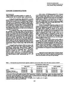
FIG. 3. A general outline of the in situ compensation method for a SQUID-based magnetometry, a case of magnetic field Hset dependent studies. This example is based on experimental data obtained at T = 5 K for a specimen S consisting of 5 nm thin (Ga,Mn)N layer (marked in red) grown on 330 µm thick sapphire substrate (grey). Panel (a) depicts results of direct measurements of the magnetic moment mexp (H) of the whole specimen (gray circles with red filling) mounted on a standard sample holder (a long Si stick, black). Apart from H ' 0 region the overwhelming majority of the flux contributing to mexp (H) comes from the bulky substrate and so this part of mexp (H) may transmit all possible, generally minute, magnetometer performance flaws, which will in turn considerably affect the outcome ascribed to the investigated layer if the substrate contribution is approximated by a linear in field term: αL Hset . When the same sample gets abutted along the length of the sample holder by strips of matching substrate material (b), then, following the consideration of the vastly enlarged symmetry of such an ”elongated” substrate, its flux nearly nulls out and the remaining net flux contributing to mexp (H) in the whole range of H comes predominantly from the (magnetic) layer of interest [red bullets, please note 20 times expanded left Y scale with respect to panel (a)]. Orange bullets represent the same data set but plotted on the same scale as in panel (a) (right Y scale). Despite the strong compensation (above 95%) this mexp (H) does not show a clear tendency to saturation, neither does the reference sapphire sample - marked by light-grey bullets, nor its signal nulls out. Both the sample and the reference are of different sizes and weights and both are not perfectly abutted by arranged in the same way compensating sapphire strips - what illustrates the typical experimental situation. Further data reduction based upon the method set by Eq. (3) allows to ambiguously establish the contribution of the magnetic layer alone. The final result is depicted in Fig. 5 (a).
strips. However, such conditions are very hard to achieve repeatedly (for example the typical spread in thickness of epi-ready semiconductor substrates approaches 30 µm, 2 – 5% relative, even for the wafers taken from the same batch). Such small discrepancies could have not been noticed in the very low field magnetometry required for those studies, simply because in weak field region the signal related to such imbalance surely fell below the magnetometer’s ultimate sensitivity. Importantly, it will be detrimental to a high precision magnetometry in the high field limits. For completeness, it has to be noted that some other methods were put forward to deal with the spurious contribution of the bulky substrates and/or bulky specimen carriers, like gelatin or particularly quartz capsules, quartz rod or tubes. The provided within the MultiVu package automated background subtraction method, although widely employed in research practice is of very limited use here since it is far too sensitive to very likely minute misplacement of the sample and its reference, and so it is prone to significant errors in the final results. Yet another approach, based on a differential method for background subtraction47 strictly relies on a perfectly symmetrical mounting of the sample and the relevant reference and the output is obtained only after a six-
parameters fitting of the measured V (z) to the elaborated by the authors relevant for the method Υ(z) function. The differential approach seems to be a plausible solution for a range of specific samples (of chemical or biological interests), however it requires the slowest possible measurement mode (the ”full scan” method) and its fidelity has not been put to a test above 2 kOe, that is well below the full extent of the magnetic field available for experiments. To complete this brief survey we note that none of the reported above method fulfills the conditions expected from precision magnetometry executed in the whole available in the MPMS magnetometers T and H ranges. Undoubtedly, the closest to such needs is the method employing abutting strips of substrate matching material38 , but in the presented form it actually represents only a concept, although successful, applied to a very particular experimental need. Therefore, a more elaborate and practically tested concept is needed to take the full advantage of this method of compensation - an approach which will not only eliminate the harmful instabilities of the magnetometer output but which will simultaneously increase the precision of very thin layers investigations even when the shapes and dimensions of their substrates do not match those of the opening created by the sub-
7 strate matching material. Below we present a full account of a method of of the in situ compensation of the magnetic signal of bulky substrates characteristic for the commonly met nanoscale magnetic materials. It constitutes a vast advance with respect to the concept presented previously38 , since it allows for investigation of samples on substrates of various, not necessarily strictly rectangular shapes, masses and compositions. The concept can become a truly versatile tool in precise magnetometry, making the results of ultimately sensitive investigations much less sensitive to typical instabilities of the measuring systems. Details on the construction as well as examples of experimentally proved final assemblies are collected in Materials and Methods. The suggested by the authors design, although quite natural, turns out also quite robust. Such assemblies as in Fig. 6 endure for quite a long time. The silent feature of Fig. 2 is that the interrogated there CSH assembly has survived intact more than two years while serving to more than a hundred measurement runs performed usually in the full envelope of the environmental parameters attainable in the MPMS magnetometers.
The experimental approach
In order to achieve the required level of the absolute experimental accuracy three sets of relevant T -, H-, and time t- dependent measurements, executed preferably along the same experimental sequence, have to be executed using the same CSH. We denote them as Li with the meaning defined below. The first two sets: (i = x) of the investigated sample (i.e. the layer on the substrate) Lx and (i = ref) of the reference sample (say, the bare substrate) Lref would be sufficient if the sample and the reference were of exactly the same shape, size and weight. Then, on the basis that the fluxes of both substrates are identical and compensated to the same degree by the abutting strips, the sought signal from the layer would be just the difference between these two measurements mx = (Lx − Lref )/γx . The shape and size correcting factor γ cannot be omitted in precision magnetometry and its relevance is discussed in Supplementary information. In practice, γ scales the magnitude of the MPMS output (obtained in the point dipole approximation) to account for the real spatial extent of the sample. Therefore, a usage of γs allows to avoid very involving numerical modeling of Υ(z) for every particular experimental configuration and its further fitting to all V (z) recorded in *.raw files in the course of the whole experimental run. Following the notation adopted previously33 MPMS output data have to be divided by a relevant γ in order to recover the correct magnitude of m. However, it is practically impossible to have so well matched both the sample and the reference without destroying the former to obtain the latter, so in the everyday practice one reference specimen serves to provide the
reference signal for a range of other samples. In this case the difference (Lx − Lref ) will contain also a small portion of the signal of the empty sample holder due to the different degrees of compensation provided by the mechanically fixed abutting strips. Therefore, a third measurement of the empty sample holder LG is needed. Practically LG is dominated by the signal exerted by the gap formed between the compensating sticks (as presented in Supplementary Figure S1), so to quantify the magnitude of sample holder contribution in the case of the nonperfect compensation, LG has to be scaled down by a factor corresponding to the degree of the ”magnetic” filling of the gap by the inserted specimens: βi = µi γi /µG γG . As above, i enumerates the investigated sample (i = x) or the reference (i = ref) and µi are their corresponding masses. Again, the correcting factors γx , γref , and γG are needed to recover the correct magnitudes of Lx , Lref and LG in an accordance with their real geometrical dimensions. Please note that µG , the mass of the missing material between the compensating strips, assumes negative magnitudes and a method of its determination is given in the Supplementary Figure S2. Accordingly, the whole correction term taking care of the sample holder contribution to mx for the case of nonidentical shapes and masses of the sample and the reference assumes the form: β=
µref γref − µx γx , µG γG
(2)
and the full expression for mx is: µx γx = Lx − Lref + βLG .
(3)
Equation (3) also holds valid when the compensating strips and the substrates of the investigated samples are made of different materials. The differences in the magnetic susceptibilities are accommodated in the experimentally established magnitudes of Li . Importantly, as laboriously verified, all the necessary values of Li needed to calculate mx come directly from the values reported by the MultiVu software in the corresponding *.dat files, providing the necessary scaling factors γi are properly applied. It is worth to stress it again that there is no need to numerically simulate the expected shape of Υ(z) for each of these complicated experimental configurations and perform involved numerical fittings to reduce the experimentally measured V (z) into m. Concerning the practical aspect of this method it can be noted that it is not as laborious as it may look at the first glance. First of all, the weight of the LG in the resulting magnitude of mx is marginal and is the smaller the more geometrical dimensions of the samples and the reference correspond to these of the gap. This causes β → 0. Therefore, it is sufficient to measure the full suite of LG measurements once and repeat them rather infrequently, say once a year, providing the experimental configuration has not been changed in the meantime. The same applies to Lref , though in this case more frequent checks are advisable due to the equal importance
8 of Lref and Lx in the determination of mx . In any case, however, any investigated T -, H-, or t-dependence for the sample calls for well-matched measurements of Lref and LG . So this method works particularly great for a range of qualitatively similar samples for which the same suite of measurements and Lref is needed - so the main experimental effort can be directed to measure Lx only, as in standard magnetometry. The improvement in data quality is exemplified in Fig. 4, where magnetization curves of various sapphire pieces investigated in the course of our studies (an arbitrary, but a representative choice of the sapphire substrates available on the market, including the same sapphire sample from Fig. 1 - sample C) are established in the CSH. In respect to the whole method these measurements are of Lref type (these are pure sapphire bits), so we do not employ Eq. (3) here. Anyway, this can only be done after a proper assessment of µG . A method of its determination is given in Supplementary Figure S2. Therefore, as in Fig. 1, a linear in Hset compensation is applied [Eq. (1)]. Because the samples are physically different, this time various coefficients αL are needed – adjusted independently for each sample to obtain a flat, field independent response at high fields at 300 K, Fig. 4 (a). Then, the same αL is applied to the data obtained at low T , Fig. 4 (b). This purely technical approach to the presentation of the results has been adopted here to underline a radically increased consistency of the data. In particular, there are no sudden ”jumps” visible (although they can still be seen during standard measurements after a high, post-measurement, numerical compensation is applied) and the results are fairly symmetrical with respect to the origin of the graphs. It is worth further noting that the scales of panels (a), (c) and (d) are five-fold expanded with respect to their counterparts in Fig. 1, meaning in particular that the in situ compensation reduces the noise level associated with V (z) reduction to m. And these are the main general technical advancements in comparison to the conventional approach (Fig. 1). The sizably reduced overall curvatures of mcomp (Hset ) at stronger fields are in fact of a lesser importance - this is actually an expected effect here. Indeed, there would be no net flux originating from a CSH with a matching sample fitted in the gap, so the m(H) should be H-independent and m(H) ≡ 0, unrespectable if Hset = Hreal , or not. The scale in panel (b) remains the same as in the corresponding panel of Fig. 1, mainly because of a strong, paramagnetic-like, response exerted by pieces A and B. Both this feature and the clear FM-like appearance in weak fields at 300 K underline the important practical issue that the available sapphire substrates differ substantially in the concentration of residual magnetically active centers or contaminations. Even the employed here CSH possesses a residual magnetic signature - we routinely register a weak remnant FM-like moment of about 0.1 – 0.2 µemu at T = 300 K, seen here for samples A, C, D, and E. This is further corroborated by an observation of an inverted ferromagnetic-like response in sample
B, indicative that this sample contains less FM-like contaminants than the central part of the CSH in which the measurement takes place. On the other hand, a single test measurement at room T proves not really sufficient – the same sample B examined further down to 2 K yielded (as well as samples A and C) a very strong, prohibitive for construction purposes, temperature dependent paramagnetic response. In this particular respect, pieces D and E look very consistent in the whole T -range, yielding relatively weak in magnitude and weakly temperature dependent magnetic response. In sum, the data collected in Fig. 4 underline the importance of a pre-selection of the most possible pristine substrate materials if the sensitive magnetic studies are planned.
Sample holder centering for the measurements.
This is one of the most important experimentexecution prerequisites which have to be observed to achieve a truly sizable boost in accuracy and repeatability of the measurements. Obviously, with the increasing level of the compensation it is progressively more difficult to properly center the CSH already containing a matching sample. All inaccuracies in the sample mounting inside the gap of the CSH and the other possible inhomogeneities, both of the shape of the substrate and/or of the investigated magnetic component, are causing strong deviations from the expected Υ(z)-like shape, as exemplified in Supplementary Figure S2 - rendering the proper centering of the sample in a standard way practically impossible. It has been found, and so is suggested, to execute the centering procedure for the empty CSH before mounting of the investigated sample. Then, no further adjustments are needed after reloading of the whole sample holder assembly with sample into the magnetometer. The inevitable distortion of measured V (z), particularly for strong compensations, is the main reason that for the whole suite of the required measurements the magnetic moment should be established in the ”linear” mode, that is when the least-squares regression of the model Υ(z) into the V (z) is performed under internally set constrains that the magnetic flux originates from the central position in the scanned window (preset for the empty CSH). Importantly, the described above procedure works well in the whole temperature range of the magnetometer, despite the well-known fact that the sample changes its location with respect to the pick-up coils upon changes of T due to the thermal contraction or expansion of the whole sample support. The effect is not by all means marginal, but well contained within Eq. (3), since the inaccuracies connected with working in the ”linear” mode are either nearly identical for Lx and Lref , and so they cancel out, or are strongly reduced by β factor for LG . This is in fact another important advantage of the proposed here method of measurements. It indeed allows to work with the results provided directly by the MultiVu software. Contrary to the differential method47 , the sam-
9 0.4
15
A B
(b) Sapphire
T = 300 K CE AD
0.2
-6
mcomp ( 10 emu )
(a) Sapphire
0.0
T=2K
10
C
5
D E
0 B
-5
-0.2
( 10-6emu )
-10 0.2 -0.4
-15 0.2
(c) 0.0 -60
(d)
-40
-20
0
20
40
Hset ( kOe )
0.0 60 -80
-60
-40
-20
0
20
40
60
80
Hset ( kOe )
FIG. 4. Magnetic field Hset dependence of a nonlinear part of the magnetic moment mcomp of a few sapphire test samples (including that presented in Fig. 1 - sample C) measured at (a) 300 and (b) 2 K, with the in situ compensation realized in the compensational sample holder [presented in Fig. 6 (c)]. All the experimentally recorded magnitudes of the magnetic moment are linearly compensated in Hset by individually adjusted for each of the sample coefficients αL [Eq. (1)] to obtain a flat H-response at 300 K. Hset are the magnitudes of magnetic field recorded in the MPMS magnetometers *.dat output files. Except for sample E at 300 K, all the curves have been recorded during one way H-sweep from positive to negatives values. Left and right pointing triangles indicate data obtained for sample E during sweeping the field down from 50 kOe and up from -50 kOe, respectively.
ple position is evaluated beforehand and firmly set at the well-defined position (z0 = 2 cm at T = 300 K) for all Lx , Lref and LG measurements, so there is no need to adjust z0 numerically by an externally executed numerical routine. We conclude this part by a notion that it is highly advisable to perform the pre-measurement centering routine always at the same temperature and at the same value of Hset . The authors choice has been 300 K and 20 kOe, respectively, the latter always ramped up from H ' 0. Actually, the data presented in Fig. 2 have been collected during the pre-measurement centering of the empty CSH, and the added value brought about by such a consecutive recording of the signal of the bare CSH at the repeatable conditions is a long term monitoring of both of the sample holder and of the whole measuring process.
EXAMPLES OF APPLICATION
The developed here method originally conceived to study single nm-thin epitaxial layers of dilute (Ga,Mn)N had been put through demanding tests and mastered during the studies of the piezoelectro-magnetic coupling in (Ga,Mn)N and its role in controlling of the single ion magnetic anisotropy of Mn3+ species in this compound by means of an external electric field43 . Using a similar CSH to that presented in Fig. 6 (b), the absolute magnitudes of magnetic saturation of 30 nm thin diluted (Ga,Mn)N layers and their low temperature mag-
netic anisotropy were established. These measurements performed in two experimental configurations: in- and out- of plane (the details of the approach permitting the orientation-dependent studies in CSH are outlined in Fig. 10 in ref.43 ) allowed to precisely establish the Mn contents of these layers (x ' 2.4%) and served as the base for quantitative numerical computation within the frame of the group theory relevant for single Mn3+ ion in wurtzite GaN, to give a full account of the effects brought about by the externally applied electric field. The all-sapphire CSH exemplified in Fig. 6 (c) has been extensively used for a precise basic magnetic characterization of the (Ga,Mn)N layers and has served already to just above a hundred of full T - and H-dependent measurement runs. In particular, it served as a basic tool for magnetic characterization of the range of (Ga,Mn)N layers prepared for the study of the role of the growth temperature on the structural and magnetic characteristics of this compound25 . In the case if this study the correctness of the established upon Eq. (3) experimental magnitudes of m, and so the whole method, was proven by an excellent agreement obtained at high field region between the experimental and theoretically calculated m(H) (cf. Fig. 13 from ref.25 ). In order to put this method into an ultimate test, a range of nominally 5 nm thin (Ga,Mn)N layers of technological (intended) Mn content between 3 and 5%48 is investigated in CSH. Results obtained for one of these layers are used in Fig. 3 to exemplify advantages of the in situ compensation concept in magnetometric studies. However, we stopped there after presenting only the bare
10 m(H) obtained for this layer and a reference sapphire substrate sample. The remaining sizable slopes in H recorded for these objects result from only a partial (although reasonable high) compensation level achieved in that particular CSH. The different signs of both m(H) (Lx and Lref in our nomenclature) indicate that the main sample has its mass µx < |µG | of this particular CSH (the opposite in sign signal of the gap dominates in this case), whereas the reference sample has µref > |µG |. Because of different masses (as well as shape correction factors) the search mx (H) for this layer cannot be established from a simple difference Lx − Lref . Eq. (3) has to be applied and the corresponding results are plotted in 5 (a) (magenta bullets). As it is seen the resulting mx (H) does not really saturate, even at strongest applied fields of about 70 kOe mx (H) retains a convex character. Figure 5 (a) shows also one more set of results. This one has been obtained for the same sample but with the magnetic field applied perpendicularly to sample plane. To allow anisotropy studies in CSH we use the concept of special specimen preparation, put forward previously to investigate paramagnetic (Ga,Mn)N epilayers (c.f. Fig. 10 in ref.43 ). The full account of these studies has reached an advanced stage of preparation for publication48 , so we limit ourselves here to admitting that a similar level of consistency has been enjoyed for all the studied layers and that this can only be achieved when the whole experimental process is carried out with the in situ compensation and the data reduction performed within the frame set by Eq. (3). Another example where precise knowledge of the absolute values of magnetic moment proves just fundamental is during investigations of structures expected to contain an antiferromagnetic AFM component, which usually exhibits a marginally weak magnetic response. In this view, CSHs have been used to study ensembles of Fe-rich, Fex Gay Nz -like nanometer-size nanocrystals NCs embedded in GaN matrix, similar to those structurally characterized previously50 . An example of the magnetic properties of such ensembles is given in Fig. 5 (b), where magnetic responses corresponding to α-Fe NCs (open symbols) and Fex Gay Nz ones (closed symbols) measured at 2 and 300 K are plotted. In this case it is not the establishment of the magnitude of the magnetic saturation of these two ensembles that defines the real technical merit of the result. The magnetic saturation in these easy saturating magnetic systems can be equally accurately established by traditional approach without the in situ compensation from the measurements performed at weak field region (H < 10 kOe), i.e. where the contribution from the substrate to the total flux exerted by the samples is only comparable to that of the NCs. The real added value by the in situ compensation and the following data manipulation sets by Eq. (3) is the establishment that the magnetic response from these two NCs system does not show high-field kink or a slope suggestive of a spin canting or a spin-flop transition characteristic to AFM systems, or at least the results establish the ab-
solute (narrow) limit within which none of these effects takes place. On the other hand, the saturation level established in this measurement allows to verify magnetic characteristics of these particular NCs obtained by other methods. A full account of this study will be published elsewhere49 . It has to be added, that the concept of the in situ compensation proves extremely useful in the studies of broad range of systems. As an example, we take a determination of a level of magnetically responsive contaminations in bulk materials. In the referred case the very same sample holder which is depicted in Fig. 6 (b) was used to compensate the bulk diamagnetism in a search for possible superconducting precipitates in samples of topological Pb0.20 Sn0.80 Te and non-topological Pb0.80 Sn0.20 Te51 . By adjusting masses of studied Pb1−y Sny Te samples, and after correcting for the low-T sapphire response, the increased resolution of the method allowed us to establish that the relative weight of precipitations that could produce a response specific to superconducting Pb or Sn was below 0.1 ppm, proving that this method can be developed further as a very sensitive characterization tool in material science.
CONCLUSIONS
In this report a thorough method for mitigating signal stability problems in commercially available SQUIDbased magnetometers has been put forward. The method is based on the in situ magnetic compensation, at the sample holder level, of the vast majority of the dominating unwanted signal of the sample substrate, bulkiness or its carrier, which normally accompanies that of the minute object of interest. Because up to two orders of magnitude smaller signal which are processed by the magnetometer, the output is much less dependable on inevitable fluctuations of some environmental variables, that otherwise detrimentally reduce the real credibility of the outcome of the standard approach to precision magnetometry. In practice two- to five-fold reduction in the absolute noise level has been observed. Practical solutions for the achievement of the adequate compensation and the proper expressions to evaluate the final results obtained in such a compensational sample holder are given. The universal form of this expression allows to practically employ one design of the compensational sample holder in investigations of a range of specimens characterized by different sizes, shapes and compositions. Importantly, the method does not require involving any modelling of the magnetometer output signal and laborious fitting. All the required inputs to calculate the absolute magnitude of the net moment of the investigated object can be taken directly from the standard magnetometers output files. The method has been implemented in MPMS SQUID magnetometers, but it is by no mean limited to this particular system. It is exemplified and put to the test on nanometer thin layers of a dilute magnetic
11
( 10 emu )
6
25
(b)
(a)
T = 2 / 300 K
-6
20
Magnetic moment, mx
4
2
-Fe NCs
15
5 nm (Ga,Mn)N xMn= 3.4%
GaN with GaxFeyNz NCs
10
T = 5 K > TC = 3.8 K
5
0
H in plane (H _| c) H in plane H perpendicular
0
-2
-5 0
20
40
60
80
Hset ( kOe )
0
20
40
60
80
Hset ( kOe )
FIG. 5. (a) An example of in- and out- of plane (bullets and squares, respectively) magnetic measurement of a 5 nm thin (Ga,Mn)N layer with the Mn content x = 3.4% established on the account of these measurements using predictions of group theoretical model of magnetic response of a single Mn3+ ion in wurtzite GaN environment. The in-plane mx (H) has been obtained on the account of Eq. (3) employing the results of the magnetic measurements performed with the in situ compensation. Both the original m(H) for the layer and of the adequate substrate reference are presented in Fig. 3 (b). The perpendicular measurements are performed and analyzed in exactly the same manner. The full account of these studies will be published elsewhere48 . (b) Magnetic responses corresponding to α-Fe (open symbols) and Fex Gay Nz nanocrystals (closed symbols) embedded in GaN matrix established at 2 and 300 K from measurements in compensational sample holder and after final data reduction according to Eq. (3), i.e. taking the magnetization curves of a reference sapphire substrate and of the empty sample holder into account. All the relevant structural characterization and the methods employed to experimentally separate contribution from these two types of nanocrystals will be given elsewhere49 .
semiconductors, without and with embedded nanocrystals. The solution given here is of a great relevance to numerous fields of material science (to a broad community), where magnetic investigations are becoming of prime importance: biophysics, organic spintronics, and in further emerging new fields dealing with topological insulators, 3D Dirac semimetals, and 2D materials. MATERIALS AND METHODS (Ga,Mn)N
5 nm thick layers of (Ga,Mn)N are deposited by molecular beam epitaxy method25,42 on GaN-buffered (2 – 3 µm) sapphire substrates (300 – 500 µm thick). High quality single phase (Ga,Mn)N layers exhibit low temperature ferromagnetic properties42,52 . However, owing to the L = 2 and S = 2 configuration of the Mn3+ species a field of the order of a few tens of kOe is required to reach the sufficient level of saturation, which would permit an establishment of Mn concentration x with a satisfactory accuracy. It has to be noted that magnetic characterization by SQUID magnetometry is practically the last resort enabling a reasonable estimation of x for a mere nanometre thin and/or magnetically diluted layers (x < 0.1). However, a caution is required, the precision of the magnetometric determination of x can be compromised by a lack of precise knowledge about Mn oxidation state. A synchrotron based X-ray absorption near-edge
spectroscopy method appears to be the most suitable for this purpose25,44,45 .
Construction details of compensational sample holders
Figure 6 (b-d) exemplifies the actual form of the compensating sample holders (CSH) considered in this report. Since our main experimental concern has been focused on thin (Ga,Mn)N layers, which are routinely, and most economically, deposited on sapphire substrates, the main designs contain the substrate-compensating strips cut from 2” sapphire wafers, panels (b) and (c) of Fig. 6. On the same token, for demanding studies of the magnetic layers grown on GaP substrates, another CSH presented in Fig. 6 (d) has got compensating strips cut from 2” GaP wafer. It is most advantageous to prepare the compensation strips from the same batch of the wafers on which the investigated material is grown. This guarantees the closest possible levels of magnetic contamination present both in the investigated sample and in the compensating strips, and so a truly effective compensation. Actually, when 2” wafers are available, four 4.5 cm long strips are needed to be cut to provide nearly full coverage of the available space sideways of the sample (two on each side of the sample). The mechanical constrains in MPMS SQUID magnetometers restrict the total length of the sample holder to less than 20 cm, and such a length, as established by numerical simulations similar to these collected in Supplementary Figure S1,
12 (a)
10 cm
SUPPLEMENTARY INFORMATION
(b) (c) (d)
FIG. 6. Examples of the sample holders made by the authors: (a) an example of a standard one or a base for (b-d) assemblies for the in situ compensation of unwanted flux of either the substrate or a bulk part of the sample. They are customized to work with Quantum Design MPMS magnetometers. In assemblies (b) and (d) the strips of the compensating materials (sapphire and GaP, respectively) differ from the material used for the supporting stick - Si, whereas in the assembly (c) all parts are made of sapphire. Most of the results presented in this report have been obtained using this particular sample holder.
is more than sufficient to compensate most of the typically used diamagnetic substrates without introducing any experimentally noticeable modifications to the sample’s V (z), and so to established magnitudes of m. The compensating strips are then glued in pairs to the supporting stick in such a way to form an opening (a gap) in the middle of the holder of a width, preferably, a bit greater than the typical width of the investigated samples. This is the place where the investigated sample is placed. Somewhat enlarged width of the gap actually easies both mounting and removing the sample from the opening, without compromising the overall performance of the CSH. In fact, Eq. (3) takes care of a lack of the perfect compensation, so a certain flexibility in this point will not do any harm. In the first two examples given in Fig. 6 the gaps are about ∼ 5.2 × 5 mm2 , i.e. a fraction of a mm wider than the typical width of the (Ga,Mn)N samples investigated in the authors’ lab. The gap in the fourth CSH is wider due to a different demands of GaPbased layers. It turns out that the role of the material serving as the mechanical support for the whole assembly is of a prime importance if precise T -dependent studies are planned. By far the most consistent performance is obtained when the supporting stick is made of the same material as the rest of the assembly. The example of such a CSH is given in Fig. 6 (c), where instead of Si, the most easily available, clean, and affordable material for this purpose, the supporting stick is made of 2 mm wide and 200 mm long sapphire strip, cut from 200×100×0.5 mm3 R-plane sapphire plate. A strongly diluted GE varnish is used to firmly join the parts. The whole assemblies are finished with a customized standard MPMS drinking straw adaptors [seen on the standard sample holder in Fig. 6 (a)], enabling an easy connection to the standard MPMS graphite probe.
S1.
The basics of the in situ compensation in SQUID magnetometers
The underlying concept of the in situ compensation of the dominating signal of the substrate arises from the fact that in these magnetometers in which the detection of the magnetic moment relies on (an axial) movement of the sample for a scan length of a few centimeters with respect to the self-balanced sensing coils, any infinitely long shape made of magnetically homogeneous material (even an iron bar) will not produce any signal. This stems from the fact that for each individual fragment of the infinite rod there exist a partner which produces a response of the same magnitude but of the opposite sign. In practice the phrase ”infinitely long” can be replaced by ”sufficiently long”, with the required length getting shorter the less magnetic is the considered material. The influence of the length of the object can be viewed as an ”ends issue”. It is illustrated in Fig. S1. We start our considerations from an ”infinitely long” homogenously magnetized rod which is divided in its center into two semi-infinite parts [Fig. S1 (a)]. In the main panel of Fig. S1 we plot the calculated SQUID responses V (z) of each individual half-rod, taking z = 0 as the center of the sensing coils (red and black solid lines for the left and right halves, respectively). Throughout the whole study we assume the sensing coils to be arranged in the second order gradiometer fashion, as in the MPMS units, and for the numerical simulation we take the gradiometer’s coils dimensions according to MPMS specification53 . It is clearly seen, that most of the signal of the individual half-rod is ”generated” at the close vicinity of the end of each of these halves, that is, at the place where the symmetry of the semi-infinite rod is the lowest. Such a resonant-like shape of V (z) is the result of the particular gradiometer configuration and the two extrema existing on each V (z) occur at the positions z = ±R, where R = 9.7 mm in MPMS magnetometer is the radius of the gradiometer coils. Actually, this is the most general rule for this kind of magnetometry - the strongest signals come from these places where the translational symmetry is reduced. Most importantly, the sum of these two V (z) nulls out everywhere, as expected for an infinite homogenous object. By exactly the same token the system picks the signal from the sample - a typical short specimen can be viewed as two symmetry breaking ends located very close to each other (at the sample length distance), whose signals mutually cancel out away from their ends (i.e. the sample). This situation is simulated in the panel (b). Here, by pushing the same halves against each other, say by 2 mm from their origin, a 4 mm long bulge is created in the overlapping area, outlined in blue. And it is only the 4 mm long muff located symmetrically with respect to
13 the center that breaks the translational symmetry of the whole structure, so its flux nulls out in the pick-up coils except only from the muff. The corresponding V (z) for each of the halves are marked in dotted lines of matching colors and their sum, the dotted blue line, indeed nulls everywhere except of the (relatively) narrow region in the vicinity of the muff. Importantly, it is exactly the same V (z) which will be induced by a 4 mm long fragment of this rod, i.e. a sample, when tripped alone through the pick-up coils.54 The dotted grey line in Fig. S1 exemplifies the ideal point-dipole V (z) of the material from which the rod is made of and its maximum value V (0) serves as the reference level for all the other curves plotted in this graph. And the comparison of the amplitudes of this V (z) and that of the 4 mm long muff explains why in the conventional magnetometry it pays to increase the linear dimensions of the investigated (homogenous) samples - it reduces the effect of flux cancellation. Certainly, the net gain in the effective flux due to extending the length of the specimen has its limit (it has to null again for the infinitely long sample) and reaches its maximum when the length of the sample approaches R.55 More general considerations concerning the influence of samples’ linear dimensions and their alignment can be found elsewhere.33,39,56,57 Both halves of the rod can also be pull apart from their joining point at the center, say, by the same 2 mm. It is illustrated in panel (c). In this case a 4 mm gap is formed (marked in green), again sizably breaking the symmetry of the rod near the center. The corresponding V (z) for the separated semi-rods are marked by dashed lines in the graph. As in the previous case, the sum of the two dependencies (green solid line) nulls everywhere except of the (relatively) narrow region close to their ends. Most importantly, this sum corresponds precisely to a V (z) of the symmetry breaking muff, but is of the opposite sign. So, both cancel each other completely. This fact constitutes the essence of the in situ compensation method which is detailed in the main part of this report.
S2.
Determination of µG
Equation 3 from the main text states that when both the investigated specimens and the reference sample(s) are so similar that β ' 0 (Eq. 2 in the main text), the contribution of the empty compensational sample holder (CSH) to the researched signal of interest mx can be neglected. But this is rather unlikely case in a long run so the full Eq. 3 has to be used on a daily basis. For this the magnitude of µG γG , that is the product of the mass of the missing material between the compensating strips and its size correcting factor has to be established. To this end we take advantage of the test m(H) measurements performed in the all-sapphire CSH with about 5.2 mm gap between the sapphire compensating strips for differing in size and weight sapphire specimens (they
are of a different origin too). Some of the corresponding mcomp (H) dependencies are presented in Fig. 4 (a) in the main part. Since at room temperature mcomp (H) at H > ∼ 0.5 T linearly depends on H in nearly all cases, a plot of αL [the coefficient required to flat out the experimental m(H), see Eq. 1 in the main text] as the function of the product of mass times γ of these specimens yields the magnitude of µG γG at the x-intercept of this dependency. The procedure is exemplified in the main panel of Fig. S2. The best assessment is obtained from the points representing specimens of very similar shapes and weights to that of the gap (' 5 × 5 mm2 in this case), since they group very close to the sought x-intercept. However, it is worth noting that the magnitudes of αL of samples which µγ differ considerably from that of the gap also fall on the same (linear) trend established by the point representing the empty CSH (µ = 0) and the rest of points close to the x-intercept (as indicated in the inset to Fig. S2), providing the proper γ is applied. There are generally three groups of points. These of αL ∼ = 0 correspond to 5 × 5 mm2 samples of the same thickness as the compensating strips, so their µγ is very close to µG γG and for them the compensation degree approaches 100%. The second group of points with αL ∼ = −0.0033 µemu/Oe corresponds also to 5 × 5 mm2 sapphire bits but of greater masses, since they are thicker, about 0.4 mm. The third group with αL ' 0.0025 µemu/Oe corresponds to ' 5 × 4 mm2 rectangular samples. The two triangles in this group mark results obtained for one of such samples which has been mounted in this about 5 × 5 mm2 CSH either with its longer side oriented along the length of CSH (the rightpointing triangle) or perpendicularly (the top-pointing one). The observed magnitudes of αL differ in both these cases, but they fall on the the same linear dependency established by the other points when proper magnitudes of γ are applied for these two configurations. We expand on the role of γ and its proper assignment with regard to the sample’s orientation in the next section of this Supplementary Information. It has to be added that in principle instead of αL one can take results of single measurements performed at one, sufficiently strong magnetic field HS , say between 20 and 50 kOe. However, such a simplification will yield a correct magnitude µG γG only when m(HS )/m(Hw ) ∼ = HS /Hw , where the weak field magnitude Hw ranges between ∼ 1 to 5 kOe, i.e. when the magnetic response of the sample is fairly proportional to H. We summarize here that when all the described above precaution are taken into account only 2–3 experimental values of αL plus that of the empty gap are practically sufficient to accurately establish µG γG .
S3.
The role of the γ factors
The problem of non-zero specimen dimensions and their influence on the strength of the coupling with pick-
14
(a) (b) (c)
FIG. S1. (Main panel) Simulations of the changes of the signal V (z) picked up by the 2nd order gradiometer for the three cases (a – c) depicted in upper part of the figure. The solid red and black lines in the graph represent individual responses of semi-infinite rods cut from a uniformly magnetized material at position z = 0, case (a). If moved together, the resulting V (z) = 0 everywhere. By shifting these halves from z = 0, by 2 mm against each other - case (b), their corresponding V (z) shift by the same amount, dashed lines in the graph of matching colors, so their sum acquires sizable amplitudes near the center (the blue dashed line), or near the bulge created by the overlapping rods. In fact case (b) corresponds to the case (a) of an infinite rod with a muff located at its center (outlined in blue). This reflects the standard situation when samples are mounted on a very long sample holder. Indeed, the dashed blue sum corresponds precisely to the computed V (z) of a 4 mm fragment of this rod, i.e. a sample, when it is tripped alone through the pick-up coils (the light blue background for the dashed blue sum). By pulling these halves away from each other, say, again by 2 mm each way from their joining point, case (c), a 4 mm wide gap is formed (green), whose magnetic response (dotted dark green line) can be obtained again as the sum of the individual V (z) of both halves after shifting them to their new starting positions (dashed lines of matching colors). Importantly, this gap-related V (z) has got exactly the same form, but is of an opposite sign to the sample-like V (z) calculated for the case (b). This effective mutual cancelation of cases (b) and (c) constitutes the basis of the active in situ compensation of chunks of supporting material (substrates) accompanying the minute objects of investigations. The dark yellow short-dashed line exemplifies a response of only a 60 mm long rod. It corresponds to the approach exercised in ref.46 . The thin grey solid line indicates the ideal point-dipole V (z) of the material from which the rods are made and its maximum value V (0) serves as the reference level for all the other curves plotted in this graph. The white background box marks the typical scanning window used in the precise magnetometry.
up coils [this affects both amplitude and the shape of the V (z)] has been recognized already very early39,56,57 and the reader can find plenty of correction factors for various experimental configurations in these papers. Correction factors cannot be omitted in the precision magnetometry conducted on typical macroscopically large samples if such is based on the MultiVu software, since the magnitude of the measured moment is established in the point object approximation, and only in this case the
size correcting factor γ = 1. The typical specimens of layered material assume areas of 20 - 30 mm2 , so a postmeasurement correction is needed to give the account for the sample’s extent along the z axis (that is along the sample holder) and perpendicularly to it (radially). Magnitudes of γ for most frequently met cuboidal shapes are listed in Table 1 of ref.33 , for the other intermediate lengths the correct values of γ can be obtained from a linear interpolation of the data in this table or from ref.39 .
15
(a)
T = 300 K
0.002
~5 × 4 mm2
0.001
330 m sapphire
0.010
a b
0.000
0.005
c
~5 × 5 mm2
L ( 10-6emu/Oe )
L ( 10-6emu/Oe )
0.003
0.000
-0.001
-0.005
-0.002
(b) 0
10
20
30
( mg )
40
50
- GG = 30.9 mg
-0.003
(c)
400 m sapphire
-0.004 25
30
35
40
45
( mg )
FIG. S2. (Main panel) Illustration of the experimental method of establishing µG γG (the product of the mass of the missing material between the compensating strips and of the ”geometrical factor” corresponding to this gap) - case of the the all-sapphire compensational sample holder CSH assembly depicted in Fig. 6 (c) in the Materials and Methods part of the main text. The searched magnitude of µG γG = −30.9 mg is indicated by the arrow. The sign ”–” reflects an opposite magnetic response of the gap between the compensating strips and a negative value should enter Eq. 3 (main text) in a case of diamagnetic compensation. Bullets represent magnitudes of coefficients αL describing the slope of the linear (high field) part of the room temperature m(H) for tested sapphire samples. The two triangles depict αL and µγ for the same rectangular ' 5×4 mm2 sapphire sample mounted in the CSH either along the longer edge (right pointing triangle) or along the shorter one (top pointing one) - this is depicted in Fig. S3. Panels (a - c) depict the shapes of the centering scans obtained using the reciprocating sample option mode of measurement in the already pre-centered CSH (the centering issue is discussed in section S4 of this Supplementary Information) with three samples of close matching µγ to that of the compensating gap. The ”Long Detrended Voltage” (brown bullets and lines) is the direct representation of V (z) with a compensation for system drifts applied. Its amplitude corresponds to the strength of the measured moment. Dark blue lines indicate point dipole ideal response function Υ(z) fitted using the linear regression mode. The established for these particular samples coefficients αL are indicated by the arrows in the main panel.
∼ 0.97 For example for a 5 × 5 mm2 square sample γ = in parallel orientation33,39 , so the necessary correction amounts to +3% and omitting it will practically invalidate the outcome of Eq. 3. Additional caution has to be exerted when it comes to investigation of irregularly shaped samples. It is because the magnitude of γ depends not only on the shape itself but also on how this shape is oriented with respect to the axis of the gradiometer z.33,39 As the rule of the thumb γ is smaller when the sample is mounted with its longer side oriented along z and greater when perpendicularly to it. This effect gets sizably magnified in a CSH. As an example we consider the case of the rectangular sample whose established magnitudes of αL are marked by the triangles in Fig. S2. The corresponding specific experimental configurations are illustrated in Fig. S3. It becomes immediately evident that placing this 4 × 5 mm2 rectangular piece in the square 5 × 5 mm2 gap in its two basic orientation: (L) with the longer side parallel to z, and (s) perpendicular to it, generates two completely different pairs of elongated voids (marked by hatched boxes) in the otherwise uniform and very long object. As dis-
cussed in section S1, the latter does not exert any flux. The magnetometer senses only an opposite flux exerted by these two pairs of voids. However, despite the fact that both pairs of voids have the same volume and that they correspond to the same material, the flux they exerts couples completely differently to the magnetometer. The two voids in the first case, Fig. S3 (L), are exclusively located at the edges of the sample holder, that is at the farthest possible distance from the z axis, so their fluxes couple stronger with the pick-up coils than the flux exerted in configuration (s) in which majority of the flux originates from the locations which are much closer to z, i.e. where the coupling is weaker, cf. Fig. 2 b in ref.33 . Now, it has to be observed that even without the compensating strips the difference in γ for these two configuration (about 1.7% for such a shape) results in the same difference in reported magnitudes of m. However, with the strips applied, the qualitatively different location of the voids in both cases increases the difference in the response to about 5.5%, i.e. it gets three times larger. In absolute numbers, an improper assignment or omission of γ may lead to an absolute error in mx as large as 10 µemu at 50 kOe, i.e. exceeding by far the
16
(s)
S
(L)
S
FIG. S3. The two experimental configurations in which the rectangular 5 × 4 mm2 sapphire sample S has been mounted in the 5 × 5 mm2 gap of the all-sapphire compensational sample holder for the determination of the ”mass” of the gap, as detailed in Fig. S2. Each of the configurations results in differently located with respect to the magnetometer axis (green dashed line) pairs of voids in sapphire, marked here by blue hatched boxes. They are the only effective sources of the magnetic flux, but despite of the equal volume they couple differently to the magnetometer pick-up coils. This may lead to differences as large as 10−5 emu at H > 50 kOe in the absolute magnitudes of the established moments for similarly shaped samples.
requirements for the precision magnetometry.
S4.
Sample holder positioning for the measurements
We start from a notion that with the increasing level of the compensation it is progressively more difficult to properly center the CSH containing a matching sample with respect to the sensing coil (i.e. in the center of the sample centering window of the MPMS software). All inaccuracies in the sample mounting inside the gap of the CSH and the other possible inhomogeneities, both of the shape of the substrate and/or of the investigated magnetic component, are causing strong deviations from the expected Υ(z)-like shape, as exemplified in panels (a-c) of Fig. S2 - rendering the proper centering of the sample in a standard way practically impossible. The best way to circumvent this serious obstacle is to execute the centering procedure for the empty CSH before mounting of the investigated sample. Then, no further adjustments are needed after reloading of the whole sample holder assembly with the sample into the magnetometer. Of course, it is advisable to run the centering scan to confirm that the specimen remains in place. However, as long as the sample transport mechanism works according to the specifications, no additional position adjustment should be made, even if the displayed V (z) in the MultiVu’s centering window assumes a fairly bizarre shape - suggestive of a relocation of the sample to a different position. Such a conclusion might be inferred particularly from the example given in Fig. S2 (a), yet post-measurements centering test of the empty CSH reconfirmed the same position of the gap, and so the proper sample location with respect to the pick-up coils. Another confirmation of the proper
centering can be occasionally obtained while running the measuring sequence when the total flux from the substrate and the gap becomes much smaller than that of the researched magnetic system (if such is investigated). This frequently happens at weak magnetic fields when the magnetic layer exhibits a sizable nonlinear behavior, characteristic for strongly interacting systems. The inevitable distortion of measured V (z), particularly for strong compensations, is the main reason that for the whole suite of the required measurements the magnetic moment should be established in the ”linear” mode, that is when the least-squares regression of the model Υ(z) into the V (z) is performed under internally set constrains that the magnetic flux originates from the central position in the scanned window (preset before mounting the specimen). It needs to be underline here that although the MPMS system provides three procedures for data reduction: a full scan algorithm, a maximum slope method, and a least-squares regression (see ref.58 and the discussion in ref.39 ), without any doubts, only the last one is suitable for reliable minute moments magnetometry.33 The issue of adequate centering of the CSH and the necessity of limiting of the data reduction exclusively to the ”linear” mode of the least-squares regression resembles the situation commonly met during hard-axis m(T, H) measurements of an anisotropic material below its anisotropy field, that is when an odd in z component considerably distorts V (z) (c.f. Fig. 4 and the discussion in ref.33 ). In both cases correct magnitudes of m yielded in such an experimental frame is assured by the strictly even character of Υ(z). This seems to be a sufficiently unique feature differentiating the sought signal coming from the centrally located sample from all other ”signals” contributing to the measured V (z). In particular, the very well obeyed linear dependence of αL on µx γx for the samples with µx γx ' µG γG , as presented in Fig. S2, strongly endorses this supposition for this experimental case. Interestingly, the described above procedure works well in the whole temperature range of the magnetometer, despite the well-known fact that the sample changes its location with respect to the pick-up coils upon changes of T due to the thermal contraction or expansion of the whole sample support. The effect is not by all means marginal, but is eliminated when the measurements are performed in the frame set by Eq. 3 (given and detailed in the main text). Concerning the absolute magnitude of this effect we note, as documented in Fig. S4, that for a CSH made of crystalline components (Si and/or sapphire) attached to the standard graphite sample rod, the sample position does not change with respect to 300 K, i.e. where the centering takes place, by more than 0.04 cm when T is reduced to 2 K and the change is less than 0.02 cm during the T -trip to 400 K. The corresponding error of m when working in the ”linear” mode for a sample off-centered by 0.04 cm amounts to about 0.2%. Such a discrepancy is prohibitive for a precise magnetometry in general, but
17 0.02
z0 ( cm )
0.01 0.00 -0.01 -0.02 -0.03 -0.04 0
100
200
300
400
T (K)
FIG. S4. A representative temperature dependence of the sample/gap position z0 in a compensational sample holder established upon the measurement of the temperature dependence of the signal exerted by the empty gap between the compensating sapphire stripes. This dependency has been established using the ”iterative” mode for the data reduction, that is the least-squares regression was freed to search for the position of the maximum in V (z).
with the in situ substrate compensation this relative error
1
2
3
4
5
6
7
8
P. Poulopoulos A. Ney and K. Baberschke, “Surface and interface magnetic moments of Co/Cu(001),” Europhys. Lett. 54, 820 (2001). M. Sawicki, D. Chiba, A. Korbecka, Yu Nishitani, J. A. Majewski, F. Matsukura, T. Dietl, and H. Ohno, “Experimental probing of the interplay between ferromagnetism and localization in (Ga,Mn)As,” Nat. Phys. 6, 22 (2010). Daichi Chiba, Naoya Shibata, and Atsushi Tsukazaki, “Co thin films deposited directly on ZnO polar surfaces,” Scientific Reports 6, 38005 (2016). L Gladczuk, K Lasek, R Puzniak, M Sawicki, P Aleshkevych, W Paszkowicz, R Minikayev, I N Demchenko, Y Syryanyy, and P Przyslupski, “Impact of organic capping layer on the magnetic anisotropy of ultrathin Co films,” Journal of Physics D: Applied Physics 50, 485002 (2017). K. Lasek, L. Gladczuk, M. Sawicki, P. Aleshkevych, and P. Przyslupski, “MgO thickness-induced spin reorientation transition in Co0.9 Fe0.1 /MgO/Co0.9 Fe0.1 structure,” Journal of Magnetism and Magnetic Materials 444, 326 – 331 (2017). Yohei Hayashi, Yuki Hibino, Fumihiro Matsukura, Kazumoto Miwa, Shimpei Ono, Takamasa Hirai, Tomohiro Koyama, Hideo Ohno, and Daichi Chiba, “Electric-field effect on magnetic anisotropy in pt/co/pd/mgo structures deposited on gaas and si substrates,” Applied Physics Express 11, 013003 (2018). M. Sawicki, O. Proselkov, C. Sliwa, P. Aleshkevych, J. Z. Domagala, J. Sadowski, and T. Dietl, “Cubic anisotropy in (Ga,Mn)As layers: Experiment and theory,” Phys. Rev. B 97, 184403 (2018). A. Sundaresan, R. Bhargavi, N. Rangarajan, U. Siddesh,
bar applies only to the uncompensated part of the specimens’ response - mainly to the magnetic layer in question, and so is perfectly acceptable. For these reasons there is no need to launch the MPMS sample ”autotracking” option - designed to compensate for sample rod thermal expansion or contraction, in particular that this option is prone to induce some instabilities when measuring very low signals.59 Secondly, the inaccuracies connected with working in the ”linear” mode are either nearly identical for both the measurements of the sample and the reference and so they cancel out, or are strongly reduced by β factor in Eq. 3. This is in fact another important advantage of the proposed here method of measurements. It indeed allows to work with the results provided directly by the MultiVu software. Contrary to the differential method47 , the sample position is evaluated beforehand and firmly set at the well-defined position (z0 = 2 cm at T = 300 K) for all three required by Eq. 3 measurements, so there is no need to adjust z0 numerically by an externally executed numerical routine. According to the gained experience it is highly advisable to perform the pre-measurement centering routine always at the same T and H. The authors choice has been 300 K and 20 kOe, respectively, the latter always ramped up from H ' 0.
9
10
11
12
13
and C. N. R. Rao, “Ferromagnetism as a universal feature of nanoparticles of the otherwise nonmagnetic oxides,” Phys. Rev. B 74, 161306 (2006). Janusz Sadowski, Jaroslaw Z. Domagala, Roland Mathieu, Andr´ as Kov´ acs, Takeshi Kasama, Rafal E. DuninBorkowski, and T. Dietl, “Formation process and superparamagnetic properties of (Mn,Ga)As nanocrystals in GaAs fabricated by annealing of (Ga,Mn)As layers with low Mn content,” Phys. Rev. B 84, 245306 (2011). Sueli H. Masunaga, Renato F. Jardim, Marcos J. Correia, and Wagner Figueiredo, “Role of dipolar interactions and volume particle size distribution on the nonmonotonic magnetic field dependence of the blocking temperature in magnetic nanoparticles,” The Journal of Physical Chemistry C 120, 765–770 (2016), https://doi.org/10.1021/acs.jpcc.5b10933. Chandana Rath, P. Mohanty, and A. Banerjee, “Magnetic properties of nanoparticles of cobalt chromite,” Journal of Magnetism and Magnetic Materials 323, 1698 – 1702 (2011). V. Augustyns, K. van Stiphout, V. Joly, T. A. L. Lima, G. Lippertz, M. Trekels, E. Men´endez, F. Kremer, U. Wahl, A. R. G. Costa, J. G. Correia, D. Banerjee, H. P. Gunnlaugsson, J. von Bardeleben, I. Vickridge, M. J. Van Bael, J. Hadermann, J. P. Ara´ ujo, K. Temst, A. Vantomme, and L. M. C. Pereira, “Evidence of tetragonal distortion as the origin of the ferromagnetic ground state in γ−Fe nanoparticles,” Phys. Rev. B 96, 174410 (2017). A. Siusys, J. Sadowski, M. Sawicki, S. Kret, T. Wojciechowski, K. Gas, W. Szuszkiewicz, A. Kaminska, and T. Story, “All-wurtzite (In,Ga)As-(Ga,Mn)As coreshell nanowires grown by molecular beam epitaxy,” Nano Let-
18
14
15
16
17
18
19
20
21
22
23
24
25
26
ters 14, 4263–4272 (2014). J. Sadowski, S. Kret, A. Siusys, T. Wojciechowski, K. Gas, M. F. Islam, C. M. Canali, and M. Sawicki, “Wurtzite (Ga,Mn)As nanowire shells with ferromagnetic properties,” Nanoscale 9, 2129–2137 (2017). D. Peddis, C. Cannas, A. Musinu, and G. Piccaluga, “Coexistence of superparmagnetism and spin-glass like magnetic ordering phenomena in a CoFe2 O4 -SiO2 nanocomposite,” The Journal of Physical Chemistry C 112, 5141– 5147 (2008). Yuanyuan Sun, Yongping Zheng, Hongzhe Pan, Jie Chen, Weili Zhang, Lin Fu, Kaiyu Zhang, Nujiang Tang, and Youwei Du, “Magnetism of graphene quantum dots,” Quantum Materials 2, 5 (2017). Yuan Liu, Nujiang Tang, Xiangang Wan, Qian Feng, Ming Li, Qinghua Xu, Fuchi Liu, and Youwei Du, “Realization of ferromagnetic graphene oxide with high magnetization by doping graphene oxide with nitrogen,” Scientific Reports 3, 2566 (2013). Yuan Liu, Yuting Shen, Litao Sun, Jincheng Li, Chang Liu, Wencai Ren, Feng Li, Libo Gao, Jie Chen, Fuchi Liu, Yuanyuan Sun, Nujiang Tang, Hui-Ming Cheng, and Youwei Du, “Elemental superdoping of graphene and carbon nanotubes,” Nature Communications 7, 10921 (2016). L M C Pereira, T Som, J Demeulemeester, M J Van Bael, K Temst, and A Vantomme, “Paramagnetism and antiferromagnetic interactions in Cr-doped GaN,” Journal of Physics: Condensed Matter 23, 346004 (2011). M. Sawicki, E. Guziewicz, M. I. Lukasiewicz, O. Proselkov, I. A. Kowalik, W. Lisowski, P. Dluzewski, A. Wittlin, M. Jaworski, A. Wolska, W. Paszkowicz, R. Jakiela, B. S. Witkowski, L. Wachnicki, M. T. Klepka, F. J. Luque, D. Arvanitis, J. W. Sobczak, M. Krawczyk, A. Jablonski, W. Stefanowicz, D. Sztenkiel, M. Godlewski, and T. Dietl, “Homogeneous and heterogeneous magnetism in (Zn,Co)O: From a random antiferromagnet to a dipolar superferromagnet by changing the growth temperature,” Phys. Rev. B 88, 085204 (2013). L M C Pereira, U Wahl, J G Correia, M J Van Bael, K Temst, A Vantomme, and J P Arajo, “Paramagnetism and antiferromagnetic interactions in single-phase Fe-implanted ZnO,” Journal of Physics: Condensed Matter 25, 416001 (2013). Bastian Henne, Verena Ney, Mariano de Souza, and Andreas Ney, “Exchange-bias-like effect of an uncompensated antiferromagnet,” Phys. Rev. B 93, 144406 (2016). V. Ney, B. Henne, J. Lumetzberger, F. Wilhelm, K. Ollefs, A. Rogalev, A. Kovacs, M. Kieschnick, and A. Ney, “Coalescence-driven magnetic order of the uncompensated antiferromagnetic Co doped ZnO,” Phys. Rev. B 94, 224405 (2016). M. Sawicki, “Magnetic properties of (Ga,Mn)As,” J. Mag. Magn. Mater. 300, 1 (2006). K. Gas, J. Z. Domagala, R. Jakiela, G. Kunert, P. Dluzewski, E. Piskorska-Hommel, W. Paszkowicz, D. Sztenkiel, M. J. Winiarski, D. Kowalska, R. Szukiewicz, T. Baraniecki, A. Miszczuk, D. Hommel, and M. Sawicki, “Impact of substrate temperature on magnetic properties of plasma-assisted molecular beam epitaxy grown (Ga,Mn)N,” Journal of Alloys and Compounds 747, 946 – 959 (2018). Piotr Bujak, Irena Kulszewicz-Bajer, Malgorzata Zagorska, Vincent Maurel, Ireneusz Wielgus, and Adam Pron, “Polymers for electronics and spintronics,”
27
28
29
30
31
32
33
34
35
36
37
38
39
40
41
Chem. Soc. Rev. 42, 8895–8999 (2013). Martin Kop´ ani, Marcel Miglierini, Adriana Lanˇcok, J´ ulius ˇ Dekan, M´ aria Caplovicov´ a, J´ an Jakubovsk´ y, Roman Boˇca, and Hedviga Mrazova, “Iron oxides in human spleen,” BioMetals 28, 913–928 (2015). Lukas Zhao, Haiming Deng, Inna Korzhovska, Zhiyi Chen, Marcin Konczykowski, Andrzej Hruban, Vadim Oganesyan, and Lia Krusin-Elbaum, “Singular robust room-temperature spin response from topological Dirac fermions,” Nature Materials 13, 580 (2014). Prithwish Dutta, Arnab Pariari, and Prabhat Mandal, “Prominent metallic surface conduction and the singular magnetic response of topological dirac fermion in threedimensional topological insulator Bi1.5 Sb0.5 Te1.7 Se1.3 ,” Scientific Reports 7, 4883 (2017). D. W. Abraham, M. M. Frank, and S. Guha, “Absence of magnetism in hafnium oxide films,” Appl. Phys. Lett. 87, 252502 (2005). M. A. Garcia, E. Fernandez Pinel, J. de la Venta, A. Quesada, V. Bouzas, J. F. Fern´ andez, J. J. Romero, M. S. Mart´ın Gonz´ alez, and J. L. Costa-Kr¨ amer, “Sources of experimental errors in the observation of nanoscale magnetism,” Journal of Applied Physics 105, 013925 (2009). L M C Pereira, J P Arajo, M J Van Bael, K Temst, and A Vantomme, “Practical limits for detection of ferromagnetism using highly sensitive magnetometry techniques,” Journal of Physics D: Applied Physics 44, 215001 (2011). M. Sawicki, W. Stefanowicz, and A. Ney, “Sensitive SQUID magnetometry for studying nanomagnetism,” Semicon. Sci. Technol. 26, 064006 (2011). A Ney, “Magnetic properties of semiconductors and substrates beyond diamagnetism studied by superconducting quantum interference device magnetometry,” Semiconductor Science and Technology 26, 064010 (2011). A. Ney, T. Kammermeier, V. Ney, K. Ollefs, and S. Ye, “Limitations of measuring small magnetic signals of samples deposited on a diamagnetic substrate,” J. Magn. Magn. Mater. 320, 3341 (2008). L M C Pereira, “Experimentally evaluating the origin of dilute magnetism in nanomaterials,” Journal of Physics D: Applied Physics 50, 393002 (2017). S. Stefanowicz, G. Kunert, C. Simserides, J. A. Majewski, W. Stefanowicz, C. Kruse, S. Figge, Tian Li, R. Jakiela, K. N. Trohidou, A. Bonanni, D. Hommel, M. Sawicki, and T. Dietl, “Phase diagram and critical behavior of a random ferromagnet Ga1−x Mnx N,” Phys. Rev. B 88, 081201(R) (2013). M. Wang, R. A. Marshall, K. W. Edmonds, A. W. Rushforth, R. P. Campion, and B. L. Gallagher, “Threedimensional Heisenberg critical behavior in the highly disordered dilute ferromagnetic semiconductor (Ga,Mn)As,” Phys. Rev. B 93, 184417 (2016). P. Stamenov and J. M. D. Coey, “Sample size, position, and structure effects on magnetization measurements using second-order gradiometer pickup coils,” Review of Scientific Instruments 77, 015106 (2006), https://doi.org/10.1063/1.2149190. W. Stefanowicz, R. Adhikari, T. Andrearczyk, B. Faina, M. Sawicki, J. A. Majewski, T. Dietl, and A. Bonanni, “Experimental determination of Rashba spin-orbit coupling in wurtzite n-GaN:Si,” Phys. Rev. B 89, 205201 (2014). R. Adhikari, M. Matzer, A. Tarazaga Mart´ın-Luengo, M. C. Scharber, and A. Bonanni, “Rashba semiconduc-
19
42
43
44
45
46
47
48
49
50
51
52
tor as spin hall material: Experimental demonstration of spin pumping in wurtzite n-GaN:Si,” Phys. Rev. B 94, 085205 (2016). G. Kunert, S. Dobkowska, Tian Li, H. Reuther, C. Kruse, S. Figge, R. Jakiela, A. Bonanni, J. Grenzer, W. Stefanowicz, J. von Borany, M. Sawicki, T. Dietl, and D. Hommel, “Ga1−x Mnx N epitaxial films with high magnetization,” Appl. Phys. Lett. 101, 022413–1 – 022413–4 (2012). D. Sztenkiel, M. Foltyn, G. P. Mazur, R. Adhikari, K. Kosiel, K. Gas, M. Zgirski, R. Kruszka, R. Jakiela, Tian Li, A. Piotrowska, A. Bonnanni, M. Sawicki, and T. Dietl, “Stretching magnetism with an electric field in a nitride semiconductor,” Nature Communications 7, 13232 (2016). A. Bonanni, M. Sawicki, T. Devillers, W. Stefanowicz, B. Faina, Tian Li, T. E. Winkler, D. Sztenkiel, A. NavarroQuezada, M. Rovezzi, R. Jakiela, A. Grois, M. Wegscheider, W. Jantsch, J. Suffczy´ nski, F. D’Acapito, A. Meingast, G. Kothleitner, and T. Dietl, “Experimental probing of exchange interactions between localized spins in the dilute magnetic insulator (Ga,Mn)N,” Phys. Rev. B 84, 035206 (2011). W. Stefanowicz, D. Sztenkiel, B. Faina, A. Grois, M. Rovezzi, T. Devillers, A. Navarro-Quezada, Tian Li, R. Jakiela, M. Sawicki, T. Dietl, and A. Bonanni, “Structural and paramagnetic properties of dilute Ga1−x Mnx N,” Phys. Rev. B 81, 235210 (2010). T. Fukumura, Zhengwu Jin, M. Kawasaki, T. Shono, T. Hasegawa, S. Koshihara, and H. Koinuma, “Magnetic properties of Mn-doped ZnO,” Appl. Phys. Lett. 78, 958 (2001). R Cabassi, F Bolzoni, and F Casoli, “Differential method for sample holder background subtraction in superconducting quantum interference device (SQUID) magnetometry,” Measurement Science and Technology 21, 035701 (2010). K. Gas, G. Kunert, P. Duewski, R. Jakiea, D. Hommel, and M. Sawicki, “The impact of Mg doped cladding layers on ferromagnetism of (Ga,Mn)N thin films,” in preparation (2018). A. Navarro-Quezada, M. Aiglinger, B. Faina, K. Gas, M. Matzer, Tian Li, R. Adhikari, M. Sawicki, and A. Bonanni, “Magnetotransport properties of phase separated (Ga,Fe)N with embedded γ’-Gay Fe4−y N nanocrystals,” in preparation (2018). A. Navarro-Quezada, T. Devillers, Tian Li, and A. Bonanni, “Planar arrays of magnetic nanocrystals embedded in GaN,” Appl. Phys. Lett. 101, 081911 (2012). G.P. Mazur, K. Dybko, A. Szczerbakow, M. Zgirski, E. Lusakowska, S. Kret, J. Korczak, T. Story, M. Sawicki, and T. Dietl, “Majorana-like excitations in a ferromagnetic topological crystalline insulator,” cond-mat , arXiv:1709.04000 (2017). M. Sawicki, T. Devillers, S. Gal¸eski, C. Simserides, S. Dobkowska, B. Faina, A. Grois, A. Navarro-Quezada, K. N. Trohidou, J. A. Majewski, T. Dietl, and A. Bo-
53
54
55
56
57
58
59
nanni, “Origin of low-temperature magnetic ordering in Ga1−x Mnx N,” Phys. Rev. B 85, 205204 (2012). Quantum Design, “Subtracting the sample holder background from dilute samples,” MPMS Application Note , 1014–213 (2002). In presented here considerations we neglect effects of radial extent of the objects on V (z). We touch upon this issue in section S3. M. E. Hayden, V. Lambinet, S. Gomis, and G. Gries, “Note: Evaluation of magnetometry data acquired from elongated samples,” Review of Scientific Instruments 88, 056106 (2017), https://doi.org/10.1063/1.4983777. A. Zieba, “Image and sample geometry effects in SQUID magnetometers,” Rev. Sci. Instrum. 64, 3357 (1993). L. L. Miller, “The response of longitudinal and transverse pickup coils to a misaligned magnetic dipole,” Rev. Sci. Instrum. 67, 3201 (1996). Quantum Design, “The regression value algorithm,” MPMS Application Note , 1014–214 (2001). F. Bolzoni, S. Giraudo, L. Lopiano, B. Bergamasco, M. Fasano, and P.R. Crippa, “Magnetic investigations of human mesencephalic neuromelanin,” Biochim. Biophys. Acta 1586, 210 (2002).
ACKNOWLEDGEMENTS
The authors acknowledge funding from the National Science Centre (Poland) through FUGA Grant DEC-2014/12/S/ST3/00549 and OPUS Grants DEC-2013/09/B/ST3/04175 and DEC2017/27/B/ST3/02470, material issues assistance of Gerd Kunert, Alberta Bonanni, Vim van Roy, and Tomasz Baraniecki, and Andrea Navarro-Quezada (ANQ) for providing samples with embedded magnetic nanocrystals. The authors are further indebted to ANQ, and A. Rushford for critical commenting on the manuscript.
AUTHOR CONTRIBUTIONS STATEMENT
Both authors on an equal basis conceived, developed, put to the tests and conducted the experiments, as well as prepared the whole manuscript.
ADDITIONAL INFORMATION
Competing interests. The authors declare no competing interests.