A Pre-Selection Routing Scheme for Virtual Circuit Networks Qiyuan Fang Adecco Technical
[email protected]
Jorge Cobb Department of Computer Science (EC 31) The University of Texas at Dallas Richardson, TX 75083-0688
[email protected]
Abstract In virtual circuit networks, the problem of routing a connection consists of selecting the best path among all the available paths between the source and destination of the connection. In this paper, we propose a path pre-selection routing scheme that not only takes the current state of each network link into account, but also considers the routing requests being issued by other nodes in the network. To do so, time is divided into periods. At each period, each node collects all its local connection requests, and broadcasts this list of requests to all nodes in the network. At the beginning of each period, all nodes apply the same path selection algorithm to choose the optimal paths for their requests from the previous period, taking into consideration the requests of all other nodes. Finding the optimal paths is formulated and solved as a linear integer optimization problem. Our algorithm outperforms a cost function routing algorithm in terms of setup blocking rates under different traffic loads and network configurations.
Ernst Leiss Department of Computer Science The University of Houston Houston, TX
[email protected]
(bandwidth, expressed in cells per second). When the VC setup message reaches an intermediate node along the selected path, a set of admission control tests are performed to decide whether the new VC, if established, can be guaranteed its requested QoS without jeopardizing the QoS guarantees to other existing VCs. If the node can satisfy the setup request, resources are then reserved at that node and the setup message is forwarded to the next node according to the routing instructions in the setup message. On the other hand, if the node is lacking resources, a teardown message is sent back to the preceding nodes along the path to release the resources reserved for the VC. If this occurs, the request is said to be blocked.
keywords: Parallel/distributed algorithms, Routing algorithms, virtual circuit networks, quality of service.
If the final admission tests at the destination node are passed, a VC acknowledgment message is sent back to the source node to confirm the establishment of the VC. Upon receiving the acknowledgment message, the application starts transmitting its packets in order over this reserved VC. When the application terminates, either the source or the destination can send a release message to the opposite node along the established VC and release the resources along the path.
1
2
Introduction
Computer networks can be classified into two basic categories: datagram networks and virtual circuit networks [1]. In datagram networks, data packets are routed individually, and may take different paths towards the destination. In virtual circuit (VC) networks, data packets are routed in order along a fixed path between the source node and the destination node. The most well-known form of a VC network is Asynchronous Transfer Mode (ATM). ATM networks offer an increased capacity to handle a wide variety of applications such as data, voice, and video with quality of service (QoS) requirements. In VC networks, the routing problem consists of selecting the best path among all the available candidate paths between the source and destination nodes. When a source node requests a VC to a destination node, the source node uses its current view of the network state and its routing algorithm to select an entire path to the destination node that appears to be capable of supporting the requested QoS. The chosen path is encoded in a connection setup message. The VC setup message is then sent over the selected path to reserve the necessary resources
Review of Previous Work
Routing decisions affect the network resource utilization and the setup blocking rate of future requests. This is because the path of a VC remains the same throughout its lifetime. Many routing algorithms for virtual circuit networks have been proposed in recent years (see [2][3][5][7][10]). The problem formulation, objective functions and solution methods cover a wide spectrum. Some researchers focus on reducing the initial setup blocking rates while others attempt to increase the utilization of the bandwidth. To simplify the studies, researchers often propose assumptions to analyze the networks theoretically. In [3], the VC routing scheme is formulated as a multicommodity network flow problem and is proven to be NP-hard. This is because the constraint set is identical to that of the multichoice multi-constrained knapsack problem [4]. Cost functions are often used to measure the availability of network links. In general, a cost function is defined in terms of the network state information, such as the sum of measured link delays or the number of hops from the source node to the destination node. Usually, the
path selection algorithm favors those paths with minimum cost. In [7], cost functions are evaluated for primary routing of permanent virtual circuits. The authors concluded that the cost metric based on an exponential function leads to a routing algorithm with optimal competitive ratio. In [10], routing algorithms are investigated where a cost function is defined in terms of the QoS information and the hop counts of a path. A source node selects a subset of minimum-hop and minimum-hop + 1 paths among all the candidate paths at the time request. From this subset of paths, a path p is selected probabilistically using the cost of the path. The multiple path routing algorithm [5] is a dynamic routing scheme whose objective is to maximize the network throughput by minimizing cell losses. They present a least-loaded path routing algorithm (also based on cost functions) [5] is to maximize throughput in fullyconnected ATM networks. The disadvantage of cost functions is that most of the cost functions lack theoretical justification. In addition, cost functions do not take the VC setup requests of other nodes into account. For example, the routing scheme routes the requests of a source based on the past network information regardless of other current requests from the rest of the nodes in the network. A node may choose a path that seems less congested at the time of the view of the network. However, some of the links in the paths may become congested because too many other nodes select the same links at the same time, resulting in a higher setup blocking rate.
3
Pre-Selection Technique
Suppose we have a network as depicted in Figure 1 and each link has 5 available channels. Let us consider the following two cases: Case 1: There are five setup requests for the 1-11 pair and no setup requests for the 2-11 pair. Case 2: There are five setup requests for the 1-11 pair and five setup requests for the 2-11 pair. If routing with a typical cost function is used, such as shortest path, the blocking rates in case 1 and case 2 are 0% and 50%, respectively. However, in case 2, if node 1 knows that there will be five setup requests for the 2-11 pair and that link 2-11 will be solely used by the 2-11 pair, node 1 can select path 1-3-4-11 to send its setup requests, resulting in a blocking rate of 0%. In other words, if a routing algorithm can predict or collect information of incoming setup requests and use it to decide the routing paths, the setup blocking rates are expected to decrease. There are several ways to learn about other nodes incoming setup requests. One way is to use historical data and build a setup request probability function. The probability function can predict the upcoming requests of a source node for the next period. The alternative is that each node holds and collects its setup requests between network
updates and then broadcast the request information as well as its link status to the rest of the network. Each node collects the broadcast information from all other nodes. At the end of the broadcast, all nodes have a complete view of the network link capacity and the requests. In this study, we select this later method. Collecting VC setup requests will delay VC setup requests by a few seconds. Thus should not not bother most users because the actual duration of communications, such as voice and video, is much longer. Users can actually benefit from the higher rate of successful setup connection so that they do not need to re-issue connection requests. In addition, the extra network traffic to carry request information is relative light because the message itself is small. The requests for a pair of source-destination can be represented by a quadruple of integers (source, destination, number of requests, virtual bandwidth class) which requires four bytes. For an ATM network depicted in Figure 1, a node requires only 52 bytes to include all of its setup requests of a single service class to the rest of the network. In an ATM network with a speed of 622 Mbps, this extra burden is negligible.
4
Network Model
A virtual circuit network is modeled as a graph where the end-systems are represented by nodes and the communication channels are represented by directed links. Let V={1,2,…,h} be the set of nodes in the graph. Let T be the total number of directed links in the network and let L={ L1, L 2 ,...,L T } be the set of directed links. The capacity of a link is defined as W. Because each QoS request demands a certain amount of bandwidth, this bandwidth can be thought of either as the peak transmission rate of the VC, “effective bandwidth” [8], or the mean traffic rate [9]. The requested bandwidth can be further divided into classes. Each class s of requests only needs a certain amount of bandwidth ws. For class s requests, a link capacity can be expressed as Cs=W/ws, i.e., Cs is the maximum number of requests from class s which can be satisfied by the link. We refer to Cs as the number of channels of class s that the link may support. Thus, the network link capacity W can be translated into a maximum number of channels Cs for class s. Below we consider a single traffic class. However, the extension to multiple classes is simple, and discussed in the conclusions. The setup requests for each source-destination (s-d) pair in a period are assumed to follow the Poisson distribution. The network updates are assumed to be synchronized and these broadcasts reach other nodes instantaneously. This is justifiable because the time to propagate routing information is small compared to the routing update period. A feasible link is defined as a physical link with channels that can be used for setting up new connections. A path consists of a sequence of adjacent feasible links. A shortest path is defined as a path between a source node
and a destination node with the minimum number of hops. Usually, several shortest paths are available for a given source-destination pairs. The available capacity of a link is the number of channels that can be used for new connections.
5
Mathematical Model
Suppose that there are m source-destination pairs in the pending request matrix, and the number of requests for the dth pair is Rd. For the dth source-destination pair, there are td shortest paths between the source node and the destination node under current network conditions. The total number of shortest paths for all pending requests is n m
(= ∑ t d ). Each shortest path uses a number of active d=1
links. An active link corresponds to a physical link which lies on one of the shortest paths of some source-destination pair. An active link set {l1, l2, … , lq} is a subset of the physical links {L1, L2, … , LT}, q ≤ T. As network link status changes, the shortest paths for a given sourcedestination pair may vary, resulting in a different set of active links. In the following discussion, we refer to an active link simply as a link, and ignore non-active links. Let Ci represent the available capacity of the ith link in the network. Let xj be the number of requests to be routed on the jth path (1≤j≤n). For the ith link in the network, the number of requests on this link cannot exceed its available capacity. n
∑ a ij x j ≤ C i
(1)
j=1
where a ij = 1 î0
if the jth path uses the i th link.
, and 1≤ i
otherwise
≤ q, 1≤j≤n.
For the dth source-destination pair, there are Rd requests and td different shortest paths. The sum of the requests to be routed on this set of paths must be equal to Rd.
so that these links are overloaded in the next period while other paths, although with the same number of hops, have extra capacities. If a source node has several shortest paths to the same destination, the traffic load distribution on these paths will be uncertain because different traffic loads may satisfy the same objective function. Furthermore, different load patterns may make some links close to saturation while others links barely loaded. When the next period comes, we may find that some source nodes have to take much longer paths to reach their destination than expected because some overcrowded links are not available to them anymore. To strike a good balance between effectiveness of the network and resource reservation for future setups, we propose an objective function which will maximize the remaining capacity of the most congested links in the network. Thus, in this paper we propose an objective function f as follows: Maximize f, where f is the minumum of n
n
n
j=1
j=1
j=1
(C1 − ∑ a1 j x j , C 2 − ∑ a 2 jx j , ... , Cq − ∑ a qj x j ) subject to Equations (2).
This objective function will force traffic load to be evenly distributed among all possible paths so that the remaining capacity of the links can reach a maximum after all requests are routed on the selected paths. We believe this optimization criterion will create a better environment for the future setup requests. The network routing problem becomes an optimization problem of maximizing several linear equations. To transform this into a linear programming (LP) problem, we introduce a new variable xn+1 which represents the maximum value of the most congested link capacity [11]. The routing optimization problem becomes Maximize xn+1 subject to n
x n +1 + ∑ a ij x j ≤ Ci j=1
n
∑bdjx j = Rd
d = 1,…,m
(2)
j=1
n
∑ b dj x j = R d
1 if jth path is one of the shortest paths for the bdj = d th source - destination pair. 0 otherwise î th
In other words, if the j path is one of the shortest paths for the dth source-destination pair, xj is part of the request Rd (xj ∈ Rd) and the coefficient bdj is 1. Otherwise, xj is not part of the request Rd and the coefficient bdj is 0. The next step is to define an objective function. There are several ways to define an objective function. One of the optimization goals is to use the least network resources. However, some links lie on the shortest paths of several s-d pairs. Source nodes may favor some paths
(3)
(4)
j=1
x≥0 and is integer, 1 ≤ j ≤ n, 1 ≤ i ≤ q, 1 ≤ d ≤ m. Next, q slack variables are introduced into the inequalities in (4) and the inequalities are changed into equations [11]. A slack variable in this case represents the remaining capacity of the link and is greater than or equal to zero. Finally, the routing problem is transformed into a linear programming (LP) problem. Maximize xn+1 subject to n
x n +1 + ∑ a ij x j + x r = C i j=1
(5)
n
∑ b dj x j = R d
(6)
requests on some congested links. As a result, the initial blocking rate is likely to be greatly reduced.
j=1
7
x≥0 and is integer, 1 ≤ i ≤ q, 1 ≤ d ≤ m, r = n+i.
6
Optimization of The Linear Programming Problem
Optimization of the integer linear programming problem is well known for the difficulty of obtaining an exact solution [12]. In general, an integer program is converted into a linear program without integer restriction. A non-integer optimal solution is found and then the closest integer solution is believed to be the best integer optimal solution. In this study, we employ the two-phase simplex algorithm and cutting plane technique to solve this integer linear problem (for more details, see [14]). In phase I of the simplex method, artificial variables, denoted xg, are introduced to each costraint in (6). n
∑ b dj x j + x g = R d
(7)
j=1
where 1 ≤ d ≤ m and g = n + 1 + q + m. The artificial variables, along with the slack variables, form an identity submatrix in the equations, which allow to quickly find a feasible solution. From this feasible solution (which contains artificial variables) the purpose is to find another feasible solution which contains no artificial variables and is a feasible solution of the original LP (5,6). To do so, a new Phase I objective function G is introduced: Maximize G = −99(x n +2+q + x n +3+q + ... + x n +1+q+m ) subject to (5) and (7). The optimal solution with G=0 is a feasible solution of the original problem (5,6). The outcome of Phase I then becomes the starting point of Phase II. The Phase II problem is the original problem (5,6). Since a feasible solution is available at the beginning of Phase II, conducting optimization operations on LP (5,6) will generate an optimal solution. The optimal solution may not be an integer solution. In this study, we apply the cutting plane method [12] to find an approximate integer optimal solution. In the final integer optimal solution, the value of xj represents the number of requests to be routed along the jth path. Since each node applies the same algorithm with the same network information at the same time, each node has the same routing path array. However, each node only takes care of the requests to be issued from itself. When the next period comes, each node will issue the requests according to the routing array it has. Because the paths are optimized with consideration of other requests in the network, setup messages can avoid sending too many
Simulation Setup
For comparison purposes, we compare out scheme against routing algorithms proposed in [10] In [10], a cost function is defined in terms of the QoS information and the hop counts of a path. A source node selects a subset of minimum-hop and minimum-hop + 1 paths among all the candidate paths at the time of network update. From this subset of paths, a path p is selected probabilistically using the path weight Wp defined as follows:
Wp ∝
Fp Hp ⋅ Lp
where Hp is the hop count of path p. Lp is a measure of the load on path p averaged over the last update period. Fp is a feasibility factor, depending on whether path p is feasible or not. The best routing scheme in [10] is referred to as sumUTIL+HOP whose path weight is defined as follows: 100 / Hp Wp = î 1 /( Lp × Hp )
Lp ≤ 0 . 01 Otherwise
where Lp is the sum of the utilization of the links on path p. The utilization of a link is the fraction of the link currently used. Routing information is updated by nodes via periodic broadcasts of the status of their outbound links during the last period. After each update, a node uses its new routing information to compute new routes to be used for incoming connections until the next broadcast. Once a call setup request arrives, the possibility that a path is chosen is directly proportional to its relative weight in the subset of the source–destination paths. A simulator SIM-1 was written in C to evaluate the setup blocking rates based on the sumUTIL+HOP cost function. Another simulator SIM-2 was coded in C to simulate the set up processes and measure the blocking rates using our proposed routing algorithm. Both routing algorithms were tested under the same network conditions and assumptions. Three sets of source-destination pairs in the simulations are given in Table 1. The third sourcedestination set in Table 1 consists of 30 randomly chosen source-destination pairs. The network characteristics are given in Table 2. Cmax is the initial capacity of the network links. The Poisson constant [13] controls the distribution of source-destination setup requests. The constant α determines both mean and standard deviation of the request lifetime which follows an exponential distribution given by the probability function p( x ) =
1 −( x / α ) e α
At the beginning of the simulation, the capacity matrix consists of all links with the initial capacity Cmax. The request matrix is populated with random numbers that
obey the Poisson distribution. The duration matrix is also flooded with random numbers following an exponential distribution. A path-finding program is run to create the routing path array. Each node gets a set of feasible paths with the number of requests that are planned to be routed on those paths. Then, the network simulators were run to simulate the actual VC connection process and count the actual blocking rates for both algorithms. The connection setup process is simulated as stated in the introduction section of the paper. If the path is available at the time of the request, a VC is considered established. If some of the channels along the path are full, the setup request is considered blocked. No rerouting effort is made for the same request. The blocking rate is defined as the total number of setup requests blocked over the total number of setup requests issued at the same time. At the end of each round of simulation, the network simulator will output the newest network capacity matrix. To make a fair comparison, the request matrix and duration matrix at the beginning of every round of simulation are identical in both algorithms.
8
Simulation Results and Performance Comparison
Figures 2, 3 and 4 show the comparison of the two routing algorithms under different traffic loads and sourcedestination plans. The vertical coordinate in the figures is the cumulative blocking rate of the whole network. The prefix S in the label legend represents the sumUTIL+HOP algorithm while the prefix P stands for the proposed algorithm. The number in the label legend is the simulation setting number shown in Table 2. For example, the S_1 curve is the simulation result of the sumUTIL+HOP algorithm under the simulation conditions of setting number 1. It is obvious that our routing algorithm outperforms sumUTIL+HOP algorithm on all different loads of network traffic. Our algorithm works very well when the network capacity is abundant. In the plan 0 – 2 configuration, the pre-selection path routing scheme has a blocking rate around 88% lower than sumUTIL+HOP in a light loaded, 30% lower in a moderately loaded, and 16% lower in a heavily loaded network. In the plan 0 – 7 configuration, the blocking rate illustrates the same trend. Our routing scheme performs better when the network has plenty of capacity and shortest paths to choose. This is because the pre-routing algorithm carefully considers network requests as a whole so that requests can select “shortest” available paths without hitting same hot links. In addition, the pre-selection path algorithm does not limit its path selection to the minimum hop + 1 subset. Choosing longer paths makes more requests get satisfied. The disadvantage of a longer path is that the connection will occupy more resources if its lifetime happens to be long. When the network is lightly loaded, each link usually has a few channels available for the next period. In this case, the disadvantage is not so obvious. Choosing longer paths will increase the successful setup rate.
Under heavy load conditions, the available links are very limited. Very often, some links are fully occupied at the beginning of the next period so that they are not available to the requests in that period. Even though the pre-selection algorithm can still find more paths to satisfy these requests, the advantage diminishes. In the worst case, if a connection chooses a much longer path and it happens to stay on the path much longer, it will consume more badly needed resources, causing performance degradation.
9
Conclusions
This paper focuses on the development of a dynamic routing algorithm for virtual circuit networks. The proposed algorithm lets each node collect and hold connection setup requests in the current period, broadcast request information at network update time, and compute best paths for the requests it holds. The requests being held are issued on the pre-selected paths in the next period. We considered the formulation of this problem as an integer linear optimization problem. A combination of the cutting plane and two-phase simplex method was used to solve this optimal path selection problem. Discrete event simulations were performed to compare the proposed algorithm with the cost function algorithm proposed in [10]. Simulation results verify that our proposed algorithm outperforms the cost function algorithm under different network traffic loads and source-destination configurations. The pre-selection algorithm is suitable for networks with abundant link capacity and the sourcedestination pairs in the network have plenty of paths to choose. Finally, we only considered a single class of traffic. For multiple classes, a simple solution is to run the optimization algorithm multiple times, once for each class. E.g., assume we have three bandwidth classes, high, medium and low. At each update interval, the optimization algorithm would be run three times, one for each class. The output of each run is a new network state with the bandwidth available for the remaining classes, which is used as input for the next run.
References [1]
C. Scheideler, “Universal Routing Strategies for Interconnection Networks”, Springer, New York, 1998 [2] C. Hou, “Routing Virtual Circuits with Timing Requirements in Virtual Path Based ATM Networks”, Proceedings of IEEE INFOCOM ’96, Conference on Computer Communications, pp.320-328, vol. 1, March 1996 [3] Y.J. Chang, J.L.C. Wu, and H.J.Ho, “Optimal Virtual Circuit Routing in Computer Networks”, IEE Proceedings of Communications, Speech and Vision, pp.625-632, vol. 139, no. 6, December 1992 [4] P. Sinha, and A. A. Zoltners, “The Multiple-Choice Knapsack Problem”, Operations Research, pp.503-515, vol.27, no.3, May-June 1979 [5] T.P. Jordan, and M.J. More, “Routing Algorithm in ATM Networks”, IEE Eleventh UK Teletrafic Symposium, 1994 [6] Y.S. Lin and J.R.Yee, “A Distributed Routing Algorithm for Virtual Circuit Data Networks”, INFOCOM ’89, Proceedings
10 9
0
8 7 6
3 5
1
13
4 2
12
11
Figure 1 Network Topology
0.5
S_1
0.45
P_1
0.4
S_2 P_2
0.35
S_3
B lo cking Rate
of the Eighth Annual Joint Conference of the IEEE Computer and Communications Societies, pp.200 – 207, vol.1, 1989 [7] R. Gawlick, C. Kalmanek and K.G. Ramakrishnan, “On-line Routing for Permanent Virtual Circuits”, Proceedings of Fourteenth Annual Joint Conference of the IEEE Computer and Communications Societies, pp.278-288, vol.1, 1995 [8] I. Matta, and A. Bestavros, “Load Profiling for Efficient Route Selection in Multi-Class Network”, Proceedings of 1997 International Conference on Network Protocals, 1997 [9] F.Y. Lin, and K. Cheng, “Virtual Path Assignment and Virtual Circuit Routing in ATM Networks”, Proceedings of Global Telecommunications Conference, GLOBECOM ’93. [10] I. Matta, and A.U. Shankar, “Dynamic Routing of RealTime Virtual Circuits”, Proceedings of 1996 International Conference on Network Protocols, November 1996 [11] K. G. Murty, “Linear Programming”, John Wiley & Sons, New York, 1983 [12] D. R. Plane and C. McMillan, Jr., “Discrete Optimization: Integer Programming and Network Analysis for Management Decisions”, Prentice-Hall, Inc., New Jersey, 1971 [13] W. H. Beyer, “CRC Handbook of Tables for Probability and Statistics”, The Chemical Rubber Co., Cleveland, 1966 [14] Q Fang, "A pre-Selection Routing Scheme for Virtual Circuit Networks", University of Houston Master's Thesis, 1999, available from the author (
[email protected]).
P_3
0.3
S_4
0.25
P_4
0.2 0.15 0.1 0.05
Table 1. Source – Destination Plan (Source, Destination) Plan 0 – 7
30 Nodes
(0-2), (1-3), (24), (3-5), (4-6), (5-7), (6-8), (79), (8-10), (911), (10-12), (11-13), (12-0), (13-1)
(0-7), (1-8), (29), (3-10), (411), (5-12), (613), (7-0), (8-1), (9-2), (10-3), (11-4), (12-5), (13-6)
(0-8), (0-11), (1-2), (1-8), (1-11), (2-3), (2-4), (3-2), (3-13), (4-2), (4-8), (5-9), (5-12), (6-0), (6-11), (7-11), (7-13), (8-4), (8-10), (9-6), (9-2), (9-13), (10-5), (10-7), (11-1), (11-9), (12-0), (126), (13-3), (13-8)
Table 2. Network Simulation Settings Poisson Interval Setting Cmax α Constant #
0
100
200
300
400
500
600
S im ulation Step 0.7
Figu re 2 Simu lation Resu lts of Plan 0-2 S_5
0.6
P_5 S_6
0.5
P_6
Blocking Rate
Plan 0 -- 2
0
S_7 0.4
P_7 S_8
0.3
P_8
0.2
Plan
1
4
15
4
15
0--2
2
6
15
4
15
0--2
3
8
15
4
15
0--2
4
10
15
4
15
0--2
5
4
15
4
15
0--7
6
6
15
4
15
0--7
7
8
15
4
15
0--7
8
10
15
4
15
0--7
9
8
10
4
15
30 nodes
10
10
10
4
15
30 nodes
11
15
10
4
15
30 nodes
0.1
0 0
100
200
300
400
500
600
Simulation Step
Figure 3 Simulation Results of Plan 0-7 0.3
S_9
0.25
P_9 S_10 P_10
Blocking Rate
0.2
S_11 P_11
0.15
0.1
0.05
0 0
100
200
300
400
Simulation Steps
Figure 4. Simulation Results of Plan 30
500
600