bioRxiv preprint first posted online Jul. 20, 2018; doi: http://dx.doi.org/10.1101/373571. The copyright holder for this preprint (which was not peer-reviewed) is the author/funder. It is made available under a CC-BY-ND 4.0 International license.
1 2 3 4 5 6 7 8 9 10 11 12 13 14 15 16 17 18 19 20 21 22 23 24 25 26
Prepared for: Brain Title: A Predictive Epilepsy Index Based on Probabilistic Classification of Interictal Spike Waveforms Jesse A. Pfammatter1*, Rachel A. Bergstrom2*, Eli P. Wallace1, Rama K. Maganti3, and Mathew V. Jones1 1
Department of Neuroscience, University of Wisconsin, 1111 Highland Avenue, Madison, WI, 53705 2
Department of Biology, Beloit College, 700 College Street, Beloit, WI 53511
3
Department of Neurology, University of Wisconsin, 1685 Highland Avenue, Madison, WI 53705 *These authors contributed equally to this manuscript Corresponding Author: Jesse Pfammatter 5505 WIMR II 1111 Highland Ave. Madison WI, 53705 email:
[email protected]
bioRxiv preprint first posted online Jul. 20, 2018; doi: http://dx.doi.org/10.1101/373571. The copyright holder for this preprint (which was not peer-reviewed) is the author/funder. It is made available under a CC-BY-ND 4.0 International license.
27 28
Abstract Quantification of interictal spikes in EEG may provide insight on epilepsy disease
29
burden, but manual quantification of spikes is time-consuming and subject to bias. We
30
present a probability-based, automated method for the classification and quantification
31
of interictal events, using EEG data from kainate- (KA) and saline- (SA) injected mice
32
several weeks post-treatment. We first detected high-amplitude events, then projected
33
event waveforms into Principal Components space and identified clusters of spike
34
morphologies using a Gaussian Mixture Model. We calculated the odds-ratio of events
35
from KA versus SA within each cluster, converted these values to probability scores,
36
P(KA), and calculated an Hourly Epilepsy Index for each animal by summing the
37
probabilities for events where the cluster P(KA) > 0.5 and dividing the resultant sum by
38
the record duration. This Index is predictive of whether an animal received an
39
epileptogenic treatment (i.e., KA), even if a seizure was never observed. We applied
40
this method to an out-of-sample dataset to assess epileptiform spike morphologies in
41
five KA animals monitored for ~1 month. The magnitude of the Index increased over
42
time in a subset of animals and revealed changes in the prevalence of epileptiform
43
(P(KA) > 0.5) spike morphologies. Importantly, in both data sets, animals that had
44
electrographic seizures also had a high Index. This analysis is fast, unbiased, and
45
provides information regarding the salience of spike morphologies for disease
46
progression. Future refinement will allow a better understanding of the definition of
47
interictal spikes in quantitative and unambiguous terms.
bioRxiv preprint first posted online Jul. 20, 2018; doi: http://dx.doi.org/10.1101/373571. The copyright holder for this preprint (which was not peer-reviewed) is the author/funder. It is made available under a CC-BY-ND 4.0 International license.
48
Keywords and Abbreviations
49
Keywords:
50
Temporal Lobe Epilepsy (TLE), kainate, automated event detection, mouse
51 52
Abbreviations:
53
EEG: electroencephalogram
54
KA: kainate
55
SA: saline
56
P(KA): probability of having received KA treatment
57
PCA: Principal Components Analysis
58
GMM: Gaussian Mixture Model
59
bioRxiv preprint first posted online Jul. 20, 2018; doi: http://dx.doi.org/10.1101/373571. The copyright holder for this preprint (which was not peer-reviewed) is the author/funder. It is made available under a CC-BY-ND 4.0 International license.
60 61
Introduction The electroencephalogram (EEG) is an essential tool for monitoring seizures,
62
diagnosing epilepsy and understanding epileptogenesis. Most EEG analysis, including
63
the scoring of seizures and interictal epileptiform events, is carried out manually by
64
trained scorers. Manual scoring is labor-intensive and prone to low interobserver
65
agreement (Webber et al., 1993) which often precludes fine-scale and quantitative
66
analysis of EEG, especially for chronic (>24 hours) recordings commonly employed in
67
clinical and research settings (Boly and Maganti, 2014; Fisher et al., 2014).
68
Adding to the challenge of EEG analysis and diagnosis in epilepsy is a relatively
69
low seizure frequency, often much less than one/day, making capturing confirmatory
70
seizure events on EEG rare (White et al., 2010). Thus, the identification and analysis of
71
subclinical, interictal events such as spikes may be important for diagnosis,
72
identification of epileptic foci and understanding the progression of epilepsy ( Cascino et
73
al., 1992; Krendl et al., 2008; Miller and Gotman, 2008; White et al., 2010; Barkmeier et
74
al., 2012; Boly and Maganti, 2014; Avoli et al., 2013; Tomlinson et al., 2016). But the
75
definition of spike-like events for subsequent manual scoring remains an area of some
76
disagreement among clinicians (Fisher et al., 2014) and researchers (Webber et al.,
77
1993; Webber and Lesser, 2017). Together with the laborious nature of manual EEG
78
analysis, this means that the frequency of interictal spiking is not typically quantified for
79
diagnostic purposes in the clinic, though there are special cases, and is underutilized in
80
epilepsy research.
81
There are many automated approaches for detecting interictal events, including
82
template-matching (Lodder et al., 2013), non-linear energy operator (NEO) detection (
bioRxiv preprint first posted online Jul. 20, 2018; doi: http://dx.doi.org/10.1101/373571. The copyright holder for this preprint (which was not peer-reviewed) is the author/funder. It is made available under a CC-BY-ND 4.0 International license.
83
Mukhopadhyay and Ray, 1998; Malik et al., 2016) wavelet filtering and line length
84
(Bergstrom et al., 2013), and neural networks (Scheuer et al., 2017) among others
85
(Wilson and Emerson, 2002). These algorithms rely in part upon a spike definition that
86
is based on expert visual analysis and are rooted in some version of the definition by
87
Chatrian et al 1974, where a spike is a transient that is clearly distinguishable from
88
background activity, with a duration from 20 to 70 ms (Chatrian et al., 1974; Noachtar
89
and Schmidt, 2010; Kane et al., 2017). Still, a universal ground truth definition of an
90
interictal spike is lacking as demonstrated in many cases where interobserver
91
agreement may be relatively low (Gerber et al., 2008; Webber et al., 1993). Further
92
careful analysis of spike and spike-like event morphology is needed to refine this
93
definition and to improve the utility of spike analysis in epilepsy.
94
Animal studies also demonstrate that spiking of some type can be present in both
95
normal and epileptic brains of rodents ( White et al., 2010; Fisher et al., 2014; Pearce et
96
al., 2014; Twele et al., 2017), making it important to identify aspects of spike-like
97
morphologies that are specifically associated with epilepsy. But differentiation of the
98
many spike types and shapes by visual or algorithmic analysis is a difficult prospect.
99
Rigorous differentiation and quantification of spikes in epileptic versus normal animals
100
could elucidate patterns of activity that shed light on spike-related mechanisms in
101
epilepsy and identification of epileptic foci while also contributing to an unbiased
102
definition of true interictal spiking activity across models of epilepsy. Given the links
103
between interictal spiking and disease progression in epilepsy (Goodin and Aminoff,
104
1984; Staley et al., 2011), quantitative understanding and differentiation between
bioRxiv preprint first posted online Jul. 20, 2018; doi: http://dx.doi.org/10.1101/373571. The copyright holder for this preprint (which was not peer-reviewed) is the author/funder. It is made available under a CC-BY-ND 4.0 International license.
105
normal and epileptiform spike-like activity is essential for future progress in epilepsy
106
research; studies in animal models are essential to this progress.
107
Classification of spikes based on waveform morphology is a promising approach
108
for differentiating events that are normal versus those that are relevant to epilepsy.
109
Indeed, spike sorting by waveform clustering has been used to tune spike-detection and
110
quantification algorithms (Nonclercq et al., 2012), to choose spike templates (Thomas et
111
al., 2016) and to identify or predict epileptic foci (Wahlberg and Lantz, 2000). A very
112
well-studied use of waveform clustering is to distinguish individual extracellularly
113
recorded action potential waveforms in order to identify neurons in single-unit
114
recordings (Souza et al., 2018). Several clustering approaches have been used across
115
these applications, including K-means clustering and affinity propagation (Thomas et al.,
116
2016), graph theoretical algorithms (Wahlberg and Lantz, 2000), and Gaussian Mixture
117
Models (GMM) (Souza et al., 2018).
118
Here we use a novel waveform-based analysis to compare spike-like events
119
recorded from mice treated with an epileptogenic insult (i.e., kainate, a model of
120
temporal lobe epilepsy (Lévesque and Avoli, 2013)) with spike-like events recorded
121
from control mice treated with saline. We identified spike-like events in both groups,
122
then projected these waveforms into a low-dimensional (3D) space using Principal
123
Components Analysis (PCA), and clustered these waveforms using a GMM. This
124
allowed us to estimate the probability distributions that characterize normal versus
125
epileptiform spike-like waveforms and to compute the probability that specific spike
126
waveforms reflect epileptiform activity. By assigning a probability score to each event
127
type, we provide a novel measure (the Hourly Epilepsy Index) for estimating the
bioRxiv preprint first posted online Jul. 20, 2018; doi: http://dx.doi.org/10.1101/373571. The copyright holder for this preprint (which was not peer-reviewed) is the author/funder. It is made available under a CC-BY-ND 4.0 International license.
128
probability that an animal is epileptic, even in the absence of observing electrographic
129
or behavioral seizures. The novel analysis thus provides rapid and unbiased insight into
130
differences among spike types in normal and epileptic animals that can be used for
131
early diagnosis of risk and serve as a biomarker of disease progression.
132
Methods
133
Animals
134
All use of animals in this manuscript conformed to the Guide for the Care and
135
Use of Laboratory Animals (2010) and was approved by the University of Wisconsin-
136
Madison Institutional Animal Care and Use Committee.
137
Animals (C57BL/6J background, ~5 weeks old) were received from Harlan
138
(Madison, WI) and housed in groups with rodent chow and water available ad libitum.
139
After ~2 weeks of acclimation, animals underwent repeated low-dose kainate (KA) or
140
saline (SA) injections (~7 weeks old) and EEG implantation and recording (~18-20
141
weeks).
142
Epilepsy Induction
143
During the injection process, when not handled, mice were individually housed in
144
enclosed ~150 cm3 acrylic cubicles with opaque sides and clear front portals with holes
145
to allow air exchange, and equipped with corn cob bedding and rodent chow. Animals
146
were then randomly assigned to KA or SA treatment, ear punched or tagged for
147
identification and weighed. Mice received a series of intraperitoneal (IP) injections
148
based on the following schedule (herein referred to as “repeated low-dose kainate”).
149
Mice in the KA group first received a 10 mg/kg (5.5 mM) dose of kainate (Tocris
150
Bioscience, UK) delivered in 1x phosphate-buffered saline (PBS) prepared from PBS
bioRxiv preprint first posted online Jul. 20, 2018; doi: http://dx.doi.org/10.1101/373571. The copyright holder for this preprint (which was not peer-reviewed) is the author/funder. It is made available under a CC-BY-ND 4.0 International license.
151
tablets (Dot Scientific, Michigan) dissolved in deionized distilled water (DDW) and filter
152
sterilized (0.22 µm, Corning, MI). Mice continued to receive injections at 2.5-5 mg/kg
153
every 20 minutes until status epilepticus (SE) occurred (4-9 injections) (Tse et al., 2014;
154
Umpierre et al., 2016). Mice in the SA group received the same schedule of sterile PBS
155
injections. Mice were considered to be in SE when displaying behavioral seizures of
156
level 4-5 on the Racine Scale (Racine, 1972) for a minimum of 30 minutes. Mice usually
157
experienced SE for 90-180 minutes and were allowed to recover spontaneously. Mice
158
were treated in cohorts of ~8 at a time, with a ratio of ~2:1, KA:SA animals. The first
159
cohort of mice received alternating 5 mg/kg and 2.5 mg/kg injections after the initial 10
160
mg /kg dose, but this schedule took longer than only 5 mg/kg injections without any
161
noticeable differences in eventual efficacy or survival, so subsequent cohorts received 5
162
mg/kg injections. Across all cohorts, mortality was 0.5 Hz) filtered with a
178
Chebyshev Type I digital filter. All analyses presented in this manuscript used a right-
179
frontal EEG channel.
180
High-amplitude Event Detection
181
To assess the severity of epilepsy in animals injected with kainate, we developed
182
a probability-based approach for the detection of epilepsy-related events (e.g. interictal
183
abnormal events like EEG spikes, seizures) and the calculation of an epilepsy severity
184
index.
185
Filtered EEG signals were normalized to using a variation of z-score
186
normalization that we term Gaussian normalization. First, we fit a Gaussian distribution
187
to the all-points histogram of each 24-hour record using the Nelder-Mead Simplex
188
(Nelder and Mead, 1965) method as implemented by the fminsearch function in Matlab.
189
We then normalized the 24-hour record by subtracting the mean from each point and
190
dividing by the standard deviation of the model fit. The resultant normalization is
191
different from the standard z-score normalization in that the mean and standard
192
deviation components are calculated from a model estimating the Gaussian
193
components of the EEG rather than empirically calculating the mean and standard
194
deviation. We employed this normalization because it adjusts the data based on the
195
normal component of the signal and is less influenced by very large and brief artifacts.
bioRxiv preprint first posted online Jul. 20, 2018; doi: http://dx.doi.org/10.1101/373571. The copyright holder for this preprint (which was not peer-reviewed) is the author/funder. It is made available under a CC-BY-ND 4.0 International license.
196
Using normalized EEG we detected high-amplitude, spike-like events using a
197
two-threshold strategy (Twyman and Macdonald, 1991). The final thresholds used in
198
this analysis were optimized to yield the largest predictive effect size (Fig. 1D). The start
199
of an event was triggered when the EEG signal rose 5 standard deviations above the
200
mean of the Gaussian fit. An event ended when the signal passed 1 standard deviation
201
below the mean. We then combined any events occurring within 0.2 seconds of one
202
another (end to start) into a single event (Kane et al., 2017). This resulted in a list of
203
events of varying duration (98% shorter than 1s, with some representing rapid spike
204
bursts) from each animal/day EEG record. We then took two seconds of signal centered
205
on the start of each event and collated events across 72 days of recording (3-4 days
206
from each of 15 KA and 7 SA animals). This resulted in a matrix with ~33000 event
207
waveforms (1024 points each) across all treatments, recording days, and animals. We
208
chose optimal high (event start) and low (event end) threshold values after a grid search
209
to investigate high values between 3 and 8, and low values between -3 and 2 and then
210
performing a t-test to compare the number of events per hour identified in SA vs. KA
211
animals (Fig. 1D).
212
Epileptiform Event Confirmation
213
We compared the output of the two-threshold detection method with output from
214
another method that has been highly cited for seizure and interictal spike detection, and
215
that also performs similarly to manual human scoring (Bergstrom et al. 2013). Spikes,
216
seizures, and other abnormal epileptiform activity were detected in normalized EEG
217
according to Bergstrom et al. (2013). The baseline was determined using the whole
218
signal. The event threshold (SF value) was set at 4.0, where spikes were defined using
bioRxiv preprint first posted online Jul. 20, 2018; doi: http://dx.doi.org/10.1101/373571. The copyright holder for this preprint (which was not peer-reviewed) is the author/funder. It is made available under a CC-BY-ND 4.0 International license.
219
a modified amplitude of 15, and seizures were defined as events greater than one
220
second in duration. To compare the two-threshold method with that of Bergstrom et al.
221
(2013), all records were represented as logical vectors where 1 indicates the presence
222
of an event during each second of recording and 0 indicates the absence of an event.
223
Confusion matrices (Fawcett, 2006) between these vectors were used to compute true-
224
positive and false-negative rates, by provisionally assuming that Bergstrom et al. (2013)
225
detected “true” events.
226
PCA, Clustering, and P(KA)
227
We performed Principal Components Analysis (PCA) (Hotelling, 1933) on the
228
matrix (~33000 x 1024) of waveforms detected by the two-threshold method and
229
projected each original waveform into the space spanned by the first three Principal
230
Components (PCs, Fig. 3). In such 3D projections, each point represents a detected
231
waveform and the distance between any two points represents the difference between
232
their original waveform shapes. Three dimensions were chosen for ease of display, but
233
higher or lower dimensional projections could be used throughout this analysis in
234
principle.
235
Waveforms that are closely intertwined with epilepsy should be a) more common
236
in KA than in SA and b) similar to other waveforms in epileptic (KA) mice and different
237
from those of SA mice. Therefore, the densities of PCA-projected points for KA and SA
238
events are expected to overlap somewhat but, by examining quantitatively their overlap
239
in specific regions of PCA space, we can compute the likelihood of a waveform in any
240
region having come from a KA vs SA animal.
bioRxiv preprint first posted online Jul. 20, 2018; doi: http://dx.doi.org/10.1101/373571. The copyright holder for this preprint (which was not peer-reviewed) is the author/funder. It is made available under a CC-BY-ND 4.0 International license.
241
The resulting ensemble of points was fit with a Gaussian Mixture Model (GMM)
242
with expectation maximization using the function fitgmdist() (McLachlan and Peel, 2005)
243
with nine components and then clustered based on the GMM coefficients. The GMM
244
defines a probability for every point in the space, and in this case reflects the prior
245
probability distribution that any waveform would be detected because both KA and SA
246
were included in the GMM fit. We then calculated the conditional probability, P(KA) that
247
events in each cluster are related to an epileptogenic treatment by computing the ratio
248
of KA (epileptogenic) to SA (control) events in each cluster (Odds ratio) and converting
249
it to a probability, P (using Odds = P / (1-P)).
250
Hourly Epilepsy Index
251
Given that there is some disagreement between manual scorers, we are
252
attempting to provide a statistical and unbiased measure of epileptiform event
253
frequencies. We first defined epileptiform event morphologies as events with a P(KA) >
254
0.50, because they are more likely to be found in KA than SA animals and are therefore
255
more relevant to epilepsy. The range of P(KA) values was rescaled from 0.5 -1.0 to 0 –
256
1, scaled P(KA) = (P(KA) - 0.5) * 2, to reflect the relative contribution of each event
257
morphology to the KA-specific set. Our method is probabilistic, so it can only be
258
interpreted as an “index” rather than an actual count of interictal events. Therefore, we
259
define an Hourly Epilepsy Index = ∑(frequency of events in each cluster with P(KA) >
260
0.5 x associated scaled P(KA)).
261
Parameter Optimization
262 263
One tunable parameter in this analysis is the choice of how many clusters to use in modeling the data (i.e., how fine-grained should our analysis of waveform shapes
bioRxiv preprint first posted online Jul. 20, 2018; doi: http://dx.doi.org/10.1101/373571. The copyright holder for this preprint (which was not peer-reviewed) is the author/funder. It is made available under a CC-BY-ND 4.0 International license.
264
be?). To investigate this parameter, we built a set of models varying the total number of
265
GMM clusters. Additionally, because creation of a GMM in our implementation is a
266
stochastic process, we rebuilt each model at 25 unique random seeds (seeds = 1
267
through 25). In total, we generated 600 Gaussian mixture models and related cluster
268
profiles, P(KA)s, and Hourly Epilepsy Indices. From each of these model sets we
269
calculated: 1) the Negative Loglikelihood of the data fit to the GMM, 2) The average
270
belongingness of each event to its assigned cluster (Cluster Belongingness, defined
271
below), 3) the effect size between SA and KA treated animals and 4) P value comparing
272
the Hourly Epilepsy Index between SA and KA treated animals. Cluster Belongingness
273
was calculated by taking the sum of squares of the set of posterior probabilities,
274
calculated with the posterior() function in Matlab, for each event and then averaged
275
across all events. For each event, these posterior probabilities (as many probabilities as
276
there are clusters) provide the likelihood of belonging to each cluster in the model and
277
these probabilities sum to one. For example, in the case of a 2 cluster model, data point
278
A may belong equally to each cluster P = (0.5, 0.5) where its Cluster Belongingness
279
equals 0.5. In contrast, data point A may belong much more strongly to one cluster over
280
another P = (0.9, 0.1) with a cluster belongingness of 0.82. Thus, a clustering model
281
with poor fit will have a low value for Cluster Belongingness.
282
Computer Programing
283
All analyses, data processing, and event classification was done in Matlab
284
(Mathworks, Natick, MA) using home-written scripts. The final version of this algorithm
285
was executed with Matlab 2017b.
286
Statistical Analysis
bioRxiv preprint first posted online Jul. 20, 2018; doi: http://dx.doi.org/10.1101/373571. The copyright holder for this preprint (which was not peer-reviewed) is the author/funder. It is made available under a CC-BY-ND 4.0 International license.
287
The usage of statistical tests and procedures used to estimate model fit
288
are indicated throughout the methods section of this manuscript. All tests and
289
statistical applications were chosen after careful consideration of data distribution
290
(e.g. normality) and independence. All statistical tests were two-tailed. The
291
researchers were not blinded or randomized to the treatments given to animals,
292
but rather treatments (KA and SA) known to cause the development of epilepsy
293
(Tse et al., 2014; Umpierre et al., 2016) were used to calculate probabilistic
294
information that went into creating the Hourly Epilepsy Index. Indeed, the design
295
of this approach was to optimize for differences between the treatments.
296
However, we feel that this approach is warranted and importantly, the clustering
297
of the events morphologies was unsupervised and thus ‘blinded’ to the treatment
298
from which each event originated.
299
Data Availability
300
Code for the algorithm used in this manuscript has been made publicly available
301
at the GitHub repository github.com/jessePfammatter/detectIISs. Code for the
302
Bergstrom et al. algorithm can be found at github.com/bergstromr/IISdetection. Data
303
available upon request.
304
Results
305
EEG Recording and Event Detection
306
We collected three days of continuous, 24-hour EEG for 15 KA and 7 SA animals
307
and normalized the records as described above. The two-threshold event detection
308
algorithm identified 25681 and 5764 events in KA- and SA-treated animals, respectively
bioRxiv preprint first posted online Jul. 20, 2018; doi: http://dx.doi.org/10.1101/373571. The copyright holder for this preprint (which was not peer-reviewed) is the author/funder. It is made available under a CC-BY-ND 4.0 International license.
309
(Fig. 1; mean ± SD event duration for KA animals = 55 ± 148 ms; for SA animals = 169
310
± 380 ms). The average number of events per hour detected in KA (23.3 ± 27.4) and SA
311
(11.5 ± 11.0) animals using this detection method was not significantly different (Fig.
312
1C, P = 0.166, t = 1.44 , df = 19.83, two-sample T-test with unequal variances). The p-
313
value for comparison of KA and SA animals was minimized by the use of the high
314
threshold of +5 and low threshold of -1, though combinations of high thresholds of four
315
or five and low thresholds of one to -2 showed low p-values relative to all other
316
combinations (Fig 1D).
317
High-amplitude Events are Epileptiform
318
To confirm that the events identified by the two-threshold method include
319
epileptiform events, the normalized EEG signal was analyzed using an event detection
320
and sorting algorithm that is validated with human spike scoring (Bergstrom et al.,
321
2013). A comparison between events detected by the two-threshold method and spikes
322
from Bergstrom et al. resulted in a true positive rate (TPR) of 0.781 and a false positive
323
rate (FPR) of 0.005. Thus, our initial detection of spikes agrees reasonably well with a
324
previous method that itself agrees well with human scoring. In a comparison of the two-
325
threshold detection method to all epileptiform events (spikes, seizures, and other low-
326
amplitude, short duration abnormal) from Bergstrom et al. (2013), the agreement
327
between the algorithms drops precipitously (Fig 2D, TPR and FPR for all events are
328
0.038 and 0.001, respectively), suggesting that the two-threshold method is selective for
329
spike-type events and does not detect low-amplitude abnormal or some seizure-like
330
events. We illustrate specific examples of agreement (Fig 2E) and disagreement (Fig
bioRxiv preprint first posted online Jul. 20, 2018; doi: http://dx.doi.org/10.1101/373571. The copyright holder for this preprint (which was not peer-reviewed) is the author/funder. It is made available under a CC-BY-ND 4.0 International license.
331
2F) between the two detection methods, highlighting that the two-threshold detection
332
method selects for high-amplitude spike- and seizure-like activity.
333
Measures Predictive of an Epileptogenic Insult.
334
Events from KA- and SA-treated animals were projected into Principal
335
Components space (Fig. 3A, first three PCs shown). We used the first three PC (76.7%
336
of the overall variance) and clustered the data into nine groups using a GMM (Fig. 3B).
337
The probability, P(KA), that a cluster morphology is relevant to epilepsy is equal to the
338
probability of that morphology being found in KA but not SA records and was calculated
339
as the odds ratio of the number of KA to SA events for each cluster. The P(KA) for four
340
of nine clusters is above 0.5 (Fig 3C, range 0.73 – 0.99), indicating that event
341
morphologies in these clusters may be specific to the KA treatment and thus related to
342
epilepsy. On average, KA animals exhibit a significantly higher average Hourly Epilepsy
343
Index than do SA animals (11.6 ± 14.6 for KA, 3.0 ± 2.0 for SA; P = 0.039, t = 2.26, df =
344
15.04, two-sample t-test with unequal variances). Two of 15 KA animals displayed
345
electrographic seizure activity in at least one recording (Fig 3D, magenta filled circles);
346
the average Hourly Epilepsy Index for these animals falls above the 75th percentile (top
347
line of box plot) of the SA hourly index. We found that there was a broad spread of
348
Hourly Epilepsy Indices across the 17 KA mice, where eight KA mice had Hourly
349
Epilepsy Indices similar to SA mice and 9 KA mice had Hourly Epilepsy Indices above
350
the 95% confidence interval of the SA Index (95% confidence interval for SA = 1.14 -
351
4.47). This interesting result is in line with published reports of varying sensitivity to
352
systemic KA injection in epileptogenesis (Tse et al., 2014; Umpierre et al., 2016).
353
Optimization of the Clustering Algorithm
bioRxiv preprint first posted online Jul. 20, 2018; doi: http://dx.doi.org/10.1101/373571. The copyright holder for this preprint (which was not peer-reviewed) is the author/funder. It is made available under a CC-BY-ND 4.0 International license.
354
To determine the optimum number of clusters to differentiate between KA- and
355
SA-specific spike morphologies, we calculated 600 repetitions of the Gaussian Mixture
356
Model used to cluster events at each unique value of 2 to 25 clusters and random seeds
357
set from 1 to 25. The Negative Loglikelihood (Fig. 4A) approaches an asymptote around
358
eight to ten clusters, suggesting the reasonable model fit in this range. Cluster
359
Belongingness (Fig. 4B) decreases across the simulation range with no clear inflection
360
point (i.e. elbow) in the data to indicate diminishing returns of increasing cluster number.
361
Effect size and p-value for the Hourly Epilepsy Index (Fig 4C and D) models indicate
362
that the effect size and the p-value reach an asymptote in a range similar to that
363
indicated by the Negative Loglikelihood results. Here, we have a fuzzy problem in terms
364
of cluster selection. We selected nine clusters for our purposes and discuss cluster
365
selection in depth in the discussion section.
366
Cluster Morphologies Match Published Characteristics of Interictal Spikes
367
We performed a preliminary waveform shape analysis by plotting individual event
368
duration vs amplitude for each cluster. In clusters where P(KA) > 0.5 (clusters one
369
through four, Fig. 5A) many events from KA-treated animals have a higher amplitude
370
than do events from the same cluster found in SA-treated animals. The majority (92%)
371
of events in these clusters for both treatment groups are shorter than 200 ms,
372
consistent with published spike definitions. This trend is not as distinct in clusters five
373
through nine, where P(KA) < 0.5. Further inspection of events in clusters one through
374
four reveals that the morphologies of these event types are more classically “spikey”
375
(short-duration events with sharp waveforms) than are events found in the remaining
376
clusters. Finally, the majority of the events identified in KA animals (88%) were found in
bioRxiv preprint first posted online Jul. 20, 2018; doi: http://dx.doi.org/10.1101/373571. The copyright holder for this preprint (which was not peer-reviewed) is the author/funder. It is made available under a CC-BY-ND 4.0 International license.
377
clusters one through four, whereas events in SA animals were equally distributed
378
among the clusters with P(KA) above (49%) and below 0.5. The average number of
379
events per hour for each cluster in SA and KA shows separation between event
380
frequency in clusters one through four but not clusters five through nine (Fig. 5B, p-
381
values reported on each graph).
382
Analysis of Out-of-Sample Data Supports the Methodology
383
We applied the clustering approach to events detected in a novel dataset of
384
longitudinal recordings from 5 KA-treated animals (Fig 6A - D, recorded on days 30 – 34
385
and 44 – 51 post-KA). The longitudinal data were projected into the same PC space as
386
the SA and KA dataset from Fig 3A and clustered according to the same parameters as
387
Fig 3 (Fig. 6A, B). All but one animal (Animal E) experienced similar, but not identical,
388
increases over time in total event rate (average for all events per hour, Fig 6C) and
389
Hourly Epilepsy Index (clusters one through four, Fig. 6D). Electrographic seizures were
390
only detected in one animal (Animal B) at days 44 and 45; this animal displayed a trend
391
toward increasing event rate and Hourly Epilepsy Index (Fig 6C-E, magenta-filled
392
circles).
393
Discussion
394
Interictal spikes are a hallmark of the epileptic brain (Fisher et al., 2014). Yet the
395
definition of an interictal spike remains somewhat nebulous, potentially biasing spike-
396
detection strategies and algorithms. Previous analyses of spikes in kainate and other
397
models of epilepsy have relied upon scoring of spikes and other interictal events to
398
differentiate between KA-treated and control animals, where more spikes are observed
399
in epileptic than in control animals ( White et al., 2010; Bergstrom et al., 2013). In these
bioRxiv preprint first posted online Jul. 20, 2018; doi: http://dx.doi.org/10.1101/373571. The copyright holder for this preprint (which was not peer-reviewed) is the author/funder. It is made available under a CC-BY-ND 4.0 International license.
400
studies, control animals also exhibit spike-type events in the EEG; however, given that
401
control (and many KA animals) animals do not proceed to have seizures, it is probable
402
that some spikes arise by a non-epileptic mechanism, including spike-like events in
403
normal brain (e.g., sharp wave ripples (Fisher et al., 2014), electrographic noise,
404
artifact, or damage associated with electrode implantation. That non-epileptiform spikes
405
may also be present in both normal and kainate-treated animals further complicates the
406
quantification of interictal spikes and thus the interpretation of nonconvulsive EEG
407
events in epilepsy and epileptogenesis.
408
Here we present a novel automated algorithm for probability-based differentiation
409
of epileptiform versus non-epileptiform spike and interictal EEG event morphologies in
410
the kainate model of TLE. Our algorithm detects interictal events and weights them in
411
an Hourly Epilepsy Index based on the likelihood that they are, indeed, relevant to
412
epilepsy (i.e., related to an epileptogenic insult (Lévesque and Avoli, 2013)). Interictal
413
events and seizures projected into PC space were clustered using a Gaussian Mixture
414
Model. We used the probability P(KA) that an event cluster was KA-specific to calculate
415
an Hourly Epilepsy Index as a weighted average of the number of events with a P(KA) >
416
0.5. This value successfully estimates the probability that a subject had received an
417
epileptogenic insult, in this case a KA injection. This algorithm can, in principle, be
418
generally applied to chronic EEG recordings from either experimental animals or human
419
patients, if a control data set is available for comparison. It can also provide rapid and
420
quantitative scoring of interictal events to predict the likelihood that a subject is at risk
421
for developing epilepsy even in the absence of observing electrographic or behavioral
422
seizures.
bioRxiv preprint first posted online Jul. 20, 2018; doi: http://dx.doi.org/10.1101/373571. The copyright holder for this preprint (which was not peer-reviewed) is the author/funder. It is made available under a CC-BY-ND 4.0 International license.
423 424
High-amplitude Event Detection is an Inclusive Starting Point Our approach to event detection using a two-threshold algorithm selected events
425
of high amplitude compared to background signal, but did not, at the outset, impose
426
limitations on event duration or morphology. This method is therefore intentionally
427
inclusive of spike and other high-amplitude, non-spike-type events that may be
428
physiologically relevant to epilepsy. Upon visual inspection of the signal and in
429
comparison to a validated seizure- and spike-detection algorithm, we found that this
430
method preferentially detects spike-type and seizure-like activity in the EEG signal (Figs
431
1 and 2), as well as other event morphologies, including artifact (Fig 3, cluster 8). That
432
our detection method primarily selects for high-amplitude events does not negate the
433
possibility that low-amplitude interictal events are relevant to epilepsy and
434
epileptogenesis. Detection and analysis of low amplitude epileptiform events is an area
435
for further inquiry (Bergstrom et al., 2013).
436
Selecting the Appropriate Number of Clusters Is Flexible and Application
437
Dependent
438
We built on prior clustering approaches for EEG by considering how spike sorting
439
may elucidate spike morphologies relevant to epilepsy and to differentiate these
440
morphologies from non-epileptiform spike-like events observed in normal rodent brains
441
(White et al., 2010; Fisher et al., 2014). The high-amplitude events identified in records
442
from SA- and KA-treated animals were projected into PCA space and then clustered
443
using a GMM with expectation maximization. Similar to spike sorting in extracellular
444
recordings (Souza et al., 2018), we found that the GMM provided a strong fit for the
445
clustering of high-amplitude events in our dataset.
bioRxiv preprint first posted online Jul. 20, 2018; doi: http://dx.doi.org/10.1101/373571. The copyright holder for this preprint (which was not peer-reviewed) is the author/funder. It is made available under a CC-BY-ND 4.0 International license.
446
Nine clusters provided adequate separation between SA and KA-treated animals,
447
though our analyses also found that this is, indeed, a fuzzy problem with many different
448
options for cluster number selection depending on the features to be extracted. Spike
449
morphology in extracellular recording is reflective of the geometry and physiological
450
properties of individual neurons. Spike morphology in EEG may be reflective of a
451
number of different parameters, including the underlying pathology of the spike, the
452
spike location, the recording montage/referencing, individual patient and recording
453
characteristics, and other features. Defining the number of clusters therefore requires
454
careful consideration to prevent over- or under-estimation of the true number of spike
455
morphologies.
456
We found that Cluster Belongingness and p-values for the separation between
457
KA vs non-KA event morphologies improve as the number of clusters increase.
458
However, very higher cluster numbers may be partitioning spike morphologies (clusters)
459
based on individual animal or recording characteristics, rather than differentiating
460
between KA and non-KA events. Selecting a smaller number (e.g. three rather than
461
nine) of clusters for analysis does not provide statistically significant separation between
462
KA and SA animals, so it is important to consider the tradeoffs in increasing and
463
decreasing the cluster number for analysis (Figure 4). Through modeling using many
464
different cluster numbers (from two to 25), we find that there is no clear “elbow” in the
465
Negative Loglikelihood or Cluster Belongingness scores across our simulations. This
466
indicates that there is not a hard and fast cluster number for this analysis. Still, we found
467
that the p-value and effect size for the epilepsy index, and the Negative Loglikelihood
468
values seemingly approached an asymptote by nine clusters (i.e. no major
bioRxiv preprint first posted online Jul. 20, 2018; doi: http://dx.doi.org/10.1101/373571. The copyright holder for this preprint (which was not peer-reviewed) is the author/funder. It is made available under a CC-BY-ND 4.0 International license.
469
improvements at higher cluster numbers). Thus, we selected nine clusters for our
470
analysis because it effectively separated KA from SA events while minimizing animal-
471
specific effects.
472
We further explored event morphologies of individual clusters by specifically
473
focusing on event amplitude and duration (Fig 5), as instructed by the descriptive spike
474
definition of Chatrian et al. (1974). Events with a P(KA) > 0.5 (clusters 1-4, more likely to
475
be found in KA than SA animals) exist within a space consistent with general definitions
476
of spikes, that is events with high amplitude and short duration (the far lower left portion
477
of the graphs in Fig 5A). As the P(KA) drops below 0.5 (clusters 5 through 9), the events
478
begin to shift toward longer, lower-amplitude characteristics. It must be noted, however,
479
that there is not a sharp demarcation in the amplitude and duration characteristics of
480
spikes above and below the cutoff of P(KA) = 0.5.
481
In applying this analysis to other models of epilepsy, we see two major
482
approaches to selecting an appropriate number of clusters, dependent upon the end
483
goal of the analysis. One approach, similar to the approach that we have taken, is to
484
identify the minimum number of clusters that provide significant separation between
485
experimental conditions or a minimum cluster number that yield clusters of visually
486
similar morphologies. A benefit to this approach would include the differentiation of
487
noise and artifact from real epileptiform activity, as we see in cluster eight (Fig 3).
488
Quantification of events could thus proceed relatively noise-free. This is similar to but
489
more specific than an approach taken by (Nonclercq et al., 2012), where spike
490
morphologies in clusters that comprise less than 5% of the total spike count are
491
removed from analysis. The considerations for a fine-scaled epilepsy index are different
bioRxiv preprint first posted online Jul. 20, 2018; doi: http://dx.doi.org/10.1101/373571. The copyright holder for this preprint (which was not peer-reviewed) is the author/funder. It is made available under a CC-BY-ND 4.0 International license.
492
than this first approach, and would instead select a larger number of clusters for a
493
higher-resolution model of epilepsy. Care must be taken, however, not to parcellate the
494
data too far, resulting in over-fitting of the model.
495
The Hourly Epilepsy Index: What it is, What it is Not
496
We have introduced an Hourly Epilepsy Index as a summary descriptive variable
497
of the likelihood of epilepsy in an individual animal, calculated as an average hourly
498
event rate weighted based on the probability that an event morphology is found in KA-
499
but not SA-treated animals. Given that kainate injection is but one model of epilepsy, we
500
cannot yet claim that this is a true model that is applicable to all epilepsy models or
501
etiologies. However, this index does begin to address some of the challenges of rodent
502
models of epilepsy, namely that not all mice that receive KA-treatment will go on to
503
develop epilepsy (Lévesque and Avoli, 2013) and low seizure frequency may make it
504
difficult to identify all epileptic mice, by providing relevant probability-based estimates of
505
likelihood of an animal being epileptic.
506
There are several features of the Hourly Epilepsy Index that indicate that this
507
may be a valuable model by which to analyze EEG data in epilepsy studies. At its
508
simplest level, the Hourly Epilepsy Index provides a more robust separation between
509
KA and SA animals than does raw event count (Fig 1C vs Fig 3D) by excluding events
510
that are not likely to be epileptiform (events where P(KA) < 0.5) and weighting the
511
remaining events (where P(KA) > 0.5) according to the probability that they are, indeed,
512
epileptiform. The relevance of this new metric is further supported by data that reveals
513
that the Hourly Epilepsy Index is significantly higher for the few KA animals with
514
electrographic seizures than the average epilepsy index of SA-treated animals (fig 3D).
bioRxiv preprint first posted online Jul. 20, 2018; doi: http://dx.doi.org/10.1101/373571. The copyright holder for this preprint (which was not peer-reviewed) is the author/funder. It is made available under a CC-BY-ND 4.0 International license.
515
In further confirmation of this, we did not observe electrographic seizure activity in SA
516
animals or KA-treated animals that fall within the 95% CI range of the Hourly Epilepsy
517
Index for SA animals. However, these data do not fully confirm that all animals
518
displaying a high Hourly Epilepsy Index have electrographic or behavioral seizures;
519
further studies are required to confirm epilepsy.
520
Cluster one (Fig 3c, 5a) is of particular interest in considering the power of spike
521
sorting by clustering for epilepsy analysis. These events are relatively infrequent across
522
records, but are highly correlated with KA treatment (P(KA) = 0.99) and are very rare in
523
SA animals. Visual inspection of these events confirms that they are, indeed, spike-like,
524
fitting into a more classical definition of an interictal spike (Chatrian et al., 1974).
525
Because these event types are almost exclusively seen in records from KA-treated
526
animals, they are weighted more strongly in the epilepsy index than are events from
527
cluster four, which show features of spiking (high amplitude, fast duration) but may also
528
cause an expert scorer to pause on their definitive identity as an interictal spike.
529
The Hourly Epilepsy Index is not without caveats, however. Kainate is a widely-
530
used model of TLE and epileptogenesis (Lévesque and Avoli, 2013), but it is only one of
531
many models. Other models, including pilocarpine, traumatic brain injury (TBI), genetic
532
or viral models of epilepsy, and kindling, rely upon different molecular mechanisms of
533
seizure induction and may therefore produce interictal events of different morphologies.
534
Ultimately, this approach may be used to produce a library of spike templates across
535
epilepsy models to further expand and refine the working definition of an interictal spike.
536
Conclusion
bioRxiv preprint first posted online Jul. 20, 2018; doi: http://dx.doi.org/10.1101/373571. The copyright holder for this preprint (which was not peer-reviewed) is the author/funder. It is made available under a CC-BY-ND 4.0 International license.
537
Clustering of interictal spike provides insight into event morphologies relevant to
538
epilepsy and epileptogenesis. Using this clustering method, we isolated epilepsy-like
539
event morphologies that were then quantified to determine the probability that a
540
particular animal is at risk for epilepsy or not, a variable which we have called the Hourly
541
Epilepsy Index. This probabilistic classification method for interictal event waveforms
542
provides a biomarker for risk and development of epilepsy, even in the absence of
543
observing electrographic or behavioral seizures. Finally, by distinguishing spike
544
morphologies that are preferentially present in the epileptic condition, we contribute to
545
an unbiased understanding of the definition of interictal spiking and interictal spike
546
morphologies, as compared with spike-like events present in the nonepileptic brain.
547
Funding: RO1 NS075366 (MVJ), DOD PR161864 (RKM)
bioRxiv preprint first posted online Jul. 20, 2018; doi: http://dx.doi.org/10.1101/373571. The copyright holder for this preprint (which was not peer-reviewed) is the author/funder. It is made available under a CC-BY-ND 4.0 International license.
548
Figure Legends
549
Figure 1. Event detection by two-threshold approach. Sample traces of events
550
identified (red) using the two-threshold method (high threshold = 5 SD above Gaussian
551
mean, low threshold = 1 SD below mean) in (A) SA- and (B) KA-injected animals. Each
552
row in A and B shows an expanded view (indicated by the blue lines) of the signal
553
directly above. (C) Average number of events per hour detected in SA (black) versus
554
KA (red) animals (P = 0.166, t = 1.44 , df = 19.83, two-sample T-test with unequal
555
variances). Circles represent the average number of events per hour for each animal
556
over 3 days of recording. Closed circles represent animals that were recorded having an
557
electrographic seizure. (D) P-values comparing the average number of events per hour
558
in SA and KA animals across a set of high and low thresholds; the p-value is minimized
559
at 5 and -1. The center mark of the box and whisker plot represents the median, while
560
the lower and upper bounds of the box represent the 25th and 75th quartiles,
561
respectively; the whiskers extend to the most extreme data points or 1.5x the
562
interquartile range.
563
Figure 2. Interictal events correspond to epileptiform activity. We compared events
564
from the two-threshold crossing method to events detected by a validated event
565
detection and classification algorithm (Bergstrom et al., 2013). Second-by-second,
566
animal-specific (SA = black, KA = red) event classification agreement (True positive
567
rate, TPR) and the rate of detection of additional events not identified in the validated
568
method (Additional events, false positive rate, FPR) for spike-type events only (A) and
569
all event types (seizures, spikes, and other low-amplitude abnormal and epileptiform
570
events, (B), with corresponding confusion matrices (spikes only C, all events D). True
bioRxiv preprint first posted online Jul. 20, 2018; doi: http://dx.doi.org/10.1101/373571. The copyright holder for this preprint (which was not peer-reviewed) is the author/funder. It is made available under a CC-BY-ND 4.0 International license.
571
positives are events detected by both the validated algorithm and the two-threshold
572
crossing method. (E) Sample true positive events for each event type, where gray is the
573
original EEG trace, green is two-threshold detection output, and black is Bergstrom et
574
al., 2013 detection output. (F) Sample events for each detection method that were not
575
detected by the other method.
576
Figure 3. Event sorting by clustering and Hourly Epilepsy Index. (A) Events detected
577
with the two-threshold crossing method, from all animals and records, and projected into
578
Principal Components space (first three PCs shown, red = KA, black = SA). (B) Events in
579
A clustered into 9 groups using a GMM with Expectation Maximization. The upper inset
580
shows a rotated and expanded view of the same plot, allowing a view of cluster 5
581
(embedded within cluster 6, which is set to 10% transparency for visualization). (C) P(KA)
582
for each cluster identified in B calculated from the relative proportion of KA to SA events,
583
presented in descending order with examples of events. (D) The average Hourly Epilepsy
584
Index (15 KA, 7 SA animals) is much higher for animals treated with KA (P = 0.039, t =
585
2.26, df = 15.04, two-sample T-test with unequal variances). The center mark of the box
586
and whisker plot represents the median, while the lower and upper bounds of the box
587
represent the 25th and 75th quartiles, respectively; the whiskers extend to the most
588
extreme data points or 1.5x the interquartile range.
589
Figure 4. Selecting an appropriate number of clusters. We repeatedly generated a
590
set of models (n = 25, random seeds set from 1:25) specifying a range of 2 to 25 clusters
591
(totaling 600 models) and calculated the (A) Negative Loglikelihood, (B) Cluster
592
Belongingness, the (C) Effect size and (D) P value of the Hourly KA Index comparing KA
593
to SA treated animals (calculated using only events where P(KA) > 0.5). These values
bioRxiv preprint first posted online Jul. 20, 2018; doi: http://dx.doi.org/10.1101/373571. The copyright holder for this preprint (which was not peer-reviewed) is the author/funder. It is made available under a CC-BY-ND 4.0 International license.
594
offer guidelines for model selection via ‘elbows’ in the data which are indicative of
595
diminishing returns in model fit. It does not appear that there is a clear best value for
596
clustering these data into discrete groups. Therefore, the cluster number must be selected
597
and evaluated based on the goal of the cluster analysis.
598
Figure 5. Characterization of individual clusters and contribution to total event
599
count. (A) Graphical distribution of each cluster’s events in EEG amplitude (x-axis) by
600
event duration (y-axis, time (s)) for events belonging to both KA (red) and SA (black).
601
Example events from each cluster type are displayed in the upper right corner of each
602
plot. For improved visualization of the majority of data, we have set the axis to exclude a
603
small amount of the most extreme data points (most notably from cluster 7). (B) The
604
average number of events per hour within each cluster for SA (black) and KA (red)
605
animals. P-values indicate the results of t-tests between KA and SA for each cluster of
606
waveform shapes.
607
Figure 6. Detection and categorization of interictal events in longitudinal data. We
608
applied our detection and categorization algorithm to longitudinal EEG records (recorded
609
days 30 – 34 and 44 – 51 post-KA) from 5 KA mice. (A) Events identified from these 5
610
animals (purple circles) projected into PCs with data from Figure 3 (black circles, SA and
611
KA data). (B) Clustering of these new data points using the same GMM coefficients and
612
clustering parameters used in Figure 3 (cluster colors correspond to those throughout
613
manuscript). The upper inset shows a rotated and expanded view of the same plot,
614
allowing a view of cluster 5 (embedded within cluster 6, which is set to 10% transparency
615
for visualization). (C) Events per hour as detected by the two-threshold method in each
616
of the 5 KA animals over time. (D) Hourly KA Index for longitudinal data set. E) Average
bioRxiv preprint first posted online Jul. 20, 2018; doi: http://dx.doi.org/10.1101/373571. The copyright holder for this preprint (which was not peer-reviewed) is the author/funder. It is made available under a CC-BY-ND 4.0 International license.
617
events per hour as detected by the two-threshold method within each cluster group. In
618
panels C-E, records with electrographic seizures are shown as filled in circles. An
619
example seizure is shown in the inset of panel D.
bioRxiv preprint first posted online Jul. 20, 2018; doi: http://dx.doi.org/10.1101/373571. The copyright holder for this preprint (which was not peer-reviewed) is the author/funder. It is made available under a CC-BY-ND 4.0 International license.
Figure 1
C
100
5 norm amp
10 m
Events Per Hour
1h
5 norm amp
P = 0.166
Animals w/ Electrograpic Seizures
B
A
120
80 60 40 20
1s
621
Low Threshold
5 norm amp
D
0
SA
KA 0.5
-3 -2 -1 0 1 2
0.4 0.3 0.2 0.1
3 4 5 6 7 8
High Threshold
0
P-value
620
bioRxiv preprint first posted online Jul. 20, 2018; doi: http://dx.doi.org/10.1101/373571. The copyright holder for this preprint (which was not peer-reviewed) is the author/funder. It is made available under a CC-BY-ND 4.0 International license.
622
Figure 2
A
B
Spikes only
1
0.8
TPR (agreement)
0.6
0.4
0
0.005
0.01
0.015
0.02
0.025
FPR (additional events)
Bergstrom et al. 2013
Spikes Event Seconds No Event Seconds Total Seconds
Two-threshold Method Event Seconds
No Event Seconds
E Spike
Total Seconds
3502 32223
4485 983 5837413 5869636
35725
5838396 5874121
TPR = 0.781
623
0.4
0.2
0.2
C
0.6
0.03
D
FPR = 0.005
Abnormal
0
Seizure
0
0.005
0.01
0.015
0.02
0.025
FPR (additional events)
All Events Bergstrom et al. 2013
TPR (agreement)
0.8
0
All Events
1
Two-threshold Method Event Seconds
No Event Seconds
Total Seconds
Event Seconds
30243
764374
794617
No Event Seconds Total Seconds
5482 35725
5074022 5079504 5808396 5874121
TPR = 0.038
FPR = 0.001
F etBergstrom 2-threshold al. 2013
10 norm amp
10 norm amp
10 norm amp
1s
4s
1s
0.03
bioRxiv preprint first posted online Jul. 20, 2018; doi: http://dx.doi.org/10.1101/373571. The copyright holder for this preprint (which was not peer-reviewed) is the author/funder. It is made available under a CC-BY-ND 4.0 International license.
624
625
Figure 3
bioRxiv preprint first posted online Jul. 20, 2018; doi: http://dx.doi.org/10.1101/373571. The copyright holder for this preprint (which was not peer-reviewed) is the author/funder. It is made available under a CC-BY-ND 4.0 International license.
Figure 4
Effect Size of Hourly KA Index
627
4.4 10
B
5
1
Belongingness
Negative Loglikelihood
A
3.55 3.5 3.45 3.4 0
C
5
10
15
20
Number of Clusters
10
9 8 7 6 5 4 3 0
5
10
15
Number of Clusters
20
25
0.8 0.6 0.4 0.2 0
25
P-value for Hourly KA Index
626
D
5
10
15
20
25
Number of Clusters
0.2 0.15 0.1 0.05
0 0
5
10
15
20
Number of Clusters
25
bioRxiv preprint first posted online Jul. 20, 2018; doi: http://dx.doi.org/10.1101/373571. The copyright holder for this preprint (which was not peer-reviewed) is the author/funder. It is made available under a CC-BY-ND 4.0 International license.
628
629
Figure 5
bioRxiv preprint first posted online Jul. 20, 2018; doi: http://dx.doi.org/10.1101/373571. The copyright holder for this preprint (which was not peer-reviewed) is the author/funder. It is made available under a CC-BY-ND 4.0 International license.
630
631
Figure 6
bioRxiv preprint first posted online Jul. 20, 2018; doi: http://dx.doi.org/10.1101/373571. The copyright holder for this preprint (which was not peer-reviewed) is the author/funder. It is made available under a CC-BY-ND 4.0 International license.
632
References
633 634
Avoli M, de Curtis M, Köhling R. Does interictal synchronization influence ictogenesis? Neuropharmacology 2013; 69: 37–44.
635 636 637
Barkmeier DT, Senador D, Leclercq K, Pai D, Hua J, Boutros NN, et al. Electrical, molecular and behavioral effects of interictal spiking in the rat. Neurobiol Dis. 2012; 47: 92–101.
638 639 640
Bergstrom RA, Choi JH, Manduca A, Shin H-S, Worrell GA, Howe CL. Automated identification of multiple seizure-related and interictal epileptiform event types in the EEG of mice. Sci Rep 2013; 3: 1483.
641 642
Boly M, Maganti R. Monitoring epilepsy in the intensive care unit: Current state of facts and potential interest of high density EEG. Brain Injury 2014; 28: 1151–1155.
643 644 645
Cascino GD, Kelly PJ, Sharbrough FW, Hulihan JF, Hirschorn KA, Trenerry MR. Longterm follow-up of stereotactic lesionectomy in partial epilepsy: predictive factors and electroencephalographic results. Epilepsia 1992; 33: 639–644.
646 647 648
Chatrian GE, Bergamini L, Dondey M, Klass DW, Lennox Buchthal M, Petersen I. A glossary of terms most commonly used by clinical electroencephalographers. Electroenceph Clin Neurophysiol 1974; 37: 538–548.
649 650
Fawcett T. An introduction to ROC analysis. Pattern Recognition Letters 2006; 27: 861– 874.
651 652
Fisher RS, Scharfman HE, deCurtis M. How can we identify ictal and interictal abnormal activity? Adv Exp Med Biol 2014; 813: 3–23.
653 654 655
Gerber PA, Chapman KE, Chung SS, Drees C, Maganti RK, Ng Y-T, et al. Interobserver agreement in the interpretation of EEG patterns in critically ill adults. J Clin Neurophysiol 2008; 25: 241–249.
656 657
Goodin DS, Aminoff MJ. Does the interictal EEG have a role in the diagnosis of epilepsy? Lancet 1984; 1: 837–839.
658 659
Hotelling H. Analysis of a complex of statistical variables into principal components. J Educ Psychol 1933; 24: 417–441.
660 661 662 663
Kane N, Acharya J, Benickzy S, Caboclo L, Finnigan S, Kaplan PW, et al. A revised glossary of terms most commonly used by clinical electroencephalographers and updated proposal for the report format of the EEG findings. Revision 2017. Clinical Neurophysiology Practice 2017; 2: 170–185.
664 665
Krendl R, Lurger S, Baumgartner C. Absolute spike frequency predicts surgical outcome in TLE with unilateral hippocampal atrophy. Neurology 2008; 71: 413–418.
bioRxiv preprint first posted online Jul. 20, 2018; doi: http://dx.doi.org/10.1101/373571. The copyright holder for this preprint (which was not peer-reviewed) is the author/funder. It is made available under a CC-BY-ND 4.0 International license.
666 667
Lévesque M, Avoli M. The kainic acid model of temporal lobe epilepsy. Neurosci Biobehav Rev 2013; 37: 2887–2899.
668 669
Lodder SS, Askamp J, van Putten MJAM. Inter-ictal spike detection using a database of smart templates. Clin Neurophysiol 2013; 124: 2328–2335.
670 671
Malik MH, Saeed M, Kamboh AM. Automatic threshold optimization in nonlinear energy operator based spike detection. IEEE; 2016. p. 774–777.
672 673
McLachlan G, Peel D. Finite Mixture Models. Hoboken, NJ, USA: John Wiley & Sons, Inc; 2005.
674 675
Miller JW, Gotman J. The meaning of interictal spikes in temporal lobe epilepsy: Should we count them? Neurology 2008; 71: 392–393.
676 677
Mukhopadhyay S, Ray GC. A new interpretation of nonlinear energy operator and its efficacy in spike detection. IEEE Trans Biomed Eng 1998; 45: 180–187.
678 679
National Research Council. Guide for the Care and Use of Laboratory Animals. National Academics Press. 2010
680 681
Nelder JA, Mead R. A Simplex Method for Function Minimization. Computer J 1965; 7: 308–313.
682
Noachtar S, Schmidt D. Introduction. Epilepsy Behav 2010; 19: 95–95.
683 684 685
Nonclercq A, Foulon M, Verheulpen D, De Cock C, Buzatu M, Mathys P, et al. Clusterbased spike detection algorithm adapts to interpatient and intrapatient variation in spike morphology. J Neurosci Meth 2012; 210: 259–265.
686 687 688
Pearce PS, Friedman D, LaFrancois JJ, Iyengar SS, Fenton AA, MacLusky NJ, et al. Spike–wave discharges in adult Sprague–Dawley rats and their implications for animal models of temporal lobe epilepsy. Epilepsy Behav 2014; 32: 121–131.
689 690
Racine RJ. Modification of seizure activity by electrical stimulation. II. Motor seizure. Electroencephalogr Clin Neurophysiol 1972; 32: 281–294.
691 692
Scheuer ML, Bagic A, Wilson SB. Spike detection: Inter-reader agreement and a statistical Turing test on a large data set. Clin Neurophysiol 2017; 128: 243–250.
693 694
Souza BC, Lopes-dos-Santos V, Bacelo J, Tort AB. Spike sorting with Gaussian mixture models. bioRxiv 2018: 248864.
695 696
Staley KJ, White A, Dudek FE. Interictal spikes: Harbingers or causes of epilepsy? Neurosci Lett 2011; 497: 247–250.
bioRxiv preprint first posted online Jul. 20, 2018; doi: http://dx.doi.org/10.1101/373571. The copyright holder for this preprint (which was not peer-reviewed) is the author/funder. It is made available under a CC-BY-ND 4.0 International license.
697 698 699
Thomas J, Jin J, Dauwels J, Cash SS, Westover MB. Clustering of Intericatal Spikes by Dynamic Time Warping and Affinity Propagation. Proc IEEE Int Conf Acoust Speech Signal Process 2016; 2016: 749–753.
700 701 702
Tomlinson SB, Bermudez C, Conley C, Brown MW, Porter BE, Marsh ED. Spatiotemporal Mapping of Interictal Spike Propagation: A Novel Methodology Applied to Pediatric Intracranial EEG Recordings. Front Neurol 2016; 7: 1881.
703 704 705 706
Tse K, Puttachary S, Beamer E, Sills GJ, Thippeswamy T. Advantages of repeated low dose against single high dose of kainate in C57BL/6J mouse model of status epilepticus: behavioral and electroencephalographic studies. PLoS ONE 2014; 9: e96622.
707 708 709
Twele F, Schidlitzki A, Töllner K, Löscher W. The intrahippocampal kainate mouse model of mesial temporal lobe epilepsy: Lack of electrographic seizure-like events in sham controls. Epilepsia Open 2017; 2: 180–187.
710 711 712
Twyman RE, Macdonald RL. Kinetic properties of the glycine receptor main- and subconductance states of mouse spinal cord neurones in culture. J Physiol (Lond.) 1991; 435: 303–331.
713 714 715 716
Umpierre AD, Bennett IV, Nebeker LD, Newell TG, Tian BB, Thomson KE, et al. Repeated low-dose kainate administration in C57BL/6J mice produces temporal lobe epilepsy pathology but infrequent spontaneous seizures. Exp Neurol 2016; 279: 116– 126.
717 718
Wahlberg P, Lantz G. Methods for robust clustering of epileptic EEG spikes. IEEE Trans Biomed Eng 2000; 47: 857–868.
719 720 721
Wallace E, Kim DY, Kim K-M, Chen S, Braden BB, Williams J, et al. Differential effects of duration of sleep fragmentation on spatial learning and synaptic plasticity in pubertal mice. Brain Res. 2015; 1615: 116–128.
722 723 724
Webber WR, Litt B, Lesser RP, Fisher RS, Bankman I. Automatic EEG spike detection: what should the computer imitate? Electroencephalogr Clin Neurophysiol 1993; 87: 364–373.
725 726
Webber WRS, Lesser RP. Automated spike detection in EEG. Clin Neurophysiol 2017; 128: 241–242.
727 728 729
White A, Williams PA, Hellier JL, Clark S, Dudek FE, Staley KJ. EEG spike activity precedes epilepsy after kainate-induced status epilepticus. Epilepsia 2010; 51: 371– 383.
730 731
Wilson SB, Emerson R. Spike detection: a review and comparison of algorithms. Clin Neurophysiol 2002; 113: 1873–1881.