A preliminary study toward an index based on ...

Ecological Indicators 20 (2012) 345–352

Contents lists available at SciVerse ScienceDirect

Ecological Indicators journal homepage: www.elsevier.com/locate/ecolind

A preliminary study toward an index based on coralligenous assemblages for the ecological status assessment of Mediterranean French coastal waters Julie Deter a,b,∗ , Pierre Descamp c , Laurent Ballesta c , Pierre Boissery d , Florian Holon c a

L’OEil d’Andromède, 7 place Cassan, 34280 Carnon, France Institut des Sciences de l’Evolution (ISEM) – UMR 5554, Université de Montpellier 2, 34095 Montpellier cedex 5, France c Andromède Océanologie, 7 place Cassan, 34280 Carnon, France d Agence de l’Eau Rhône-Méditerranée-Corse, Délégation de Marseille, Immeuble le Noailles, 62 La Canebière, 13001 Marseille, France b

a r t i c l e

i n f o

Article history: Received 29 November 2011 Received in revised form 27 February 2012 Accepted 1 March 2012 Keywords: Coralligene Water framework directive Water quality Hard bottom assemblage ecological indicator

a b s t r a c t Despite the great contribution of coralligenous communities to Mediterranean biodiversity (second key-ecosystem after Posidonia oceanica meadows), they were never considered in the establishment of multimetric indices for ecological status assessment of marine environment. In this paper, we describe a method to evaluate the ecological status of coralligenous assemblages along Mediterranean French coasts. Several metrics were selected from literature for coralligenous assemblage description and include functional and structural information: percent cover of visible non-vagile species (using photographic quadrats along a transect) and gorgonian demography. Thirty eight field stations were sampled for these metrics in PACA (Provence-Alpes-Côte-d’Azur) region in June 2010 and considered for their morphology (bank, rim), geographical orientation and principal current direction (North, East, West, South) and depth (from −30 to −84 m). Metrics found to be linked to human pressures using ANCOVA and multiple correlation matrix were selected to be included in the index. The index (Coralligenous Assemblage Index, CAI) that we proposed was based on three selected metrics (Bryozoa percent cover, sludge percent cover, builder species percent cover) and considers depth; it was positively and significantly linked to anthropization (related to water quality). The 38 stations studied with theoretically good to bad environmental conditions were classified in levels of status in accordance with our field work knowledge. CAI variation was validated with three stations sampled with 30 other photos. This index could be an effective tool for the assessment of the ecological quality of coralligenous communities. It could be applied in the context of the Marine Strategy Framework Directive as well as in conservation and sustainable management of the marine environment. © 2012 Elsevier Ltd. All rights reserved.

1. Introduction Coralligenous concretions are primarily produced by the accumulation of encrusting algae growing at low light levels and secondarily by bio-constructor animals as polychaetes, bryozoans and gorgonians; they represent the unique calcareous formations of biogenic origin in Mediterranean Sea (Ballesteros, 2006). The resulting complex structure allows the development of a patchwork of communities dominated by living algae, suspension feeders, borers or soft-bottom fauna (in the sediment within cavities). Two main morphologies can be distinguished (Ballesteros,

∗ Corresponding author at: L’œil d’andromède, 7, place Cassan, 34280 Carnon, France. Tel.: +33 4 67 66 32 48. E-mail addresses: [email protected] (J. Deter), [email protected] (P. Descamp), [email protected] (L. Ballesta), [email protected] (P. Boissery), fl[email protected] (F. Holon). 1470-160X/$ – see front matter © 2012 Elsevier Ltd. All rights reserved. doi:10.1016/j.ecolind.2012.03.001

2006) for coralligenous frameworks: banks (built over more or less horizontal substrata) and rims (in the outer part of marine caves and on vertical cliffs). In terms of richness, biomass and production, coralligenous assemblage value is high and comparable to tropical reef assemblages (Bianchi, 2001). The other side of the coin is the important attract exerted over divers and fishermen and their damaging consequences (Ballesteros, 2006). Moreover, submarine outfalls (with their urban and industrial discharges) are widespread along the coast and rocky coasts are among the most vulnerable habitats to pollution, increased sediment loads and deposition (Airoldi, 2003; Ballesteros, 2006). Increasing anthropogenic pressures and their consequences on water quality decline have led the European Union to engage a new strategy to conserve and recover the ecological quality of the marine environment. With the Water Framework Directive (WFD, Directive 2008/56/EC), European commission aims to achieve (or maintain at least) a “good status” in all the European waters by 2015. WFD defines the ecological status as the quality of the structure and functioning of ecosystems associated with homogenous water bodies. The

346

J. Deter et al. / Ecological Indicators 20 (2012) 345–352

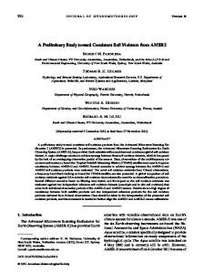
Fig. 1. Map presenting the 38 stations studied on the Mediterranean French coast (PACA region).

status of each water body is evaluated thanks to variables relative to organisms or groups of organisms sensitive to anthropogenic pressures and called biological quality elements (phytoplankton, macroalgae, angiosperms and benthic fauna) (Devlin et al., 2007). Despite the great contribution of coralligenous communities to Mediterranean biodiversity (Ballesteros, 2006) and its recognition as a natural habitat of communitarian interest, whose conservation requires the designation of Zones of Special Conservation at European level (92/43/CE Habitat Directive, habitat code 1170-14: Reefs, coralligenous assemblage), coralligenous assemblages were largely neglected for the water body quality assessment. Actually, most efforts in ecological status assessment of marine waters have been carried out in the implementation of angiosperms and soft bottom biotic indices (Borja et al., 2000; de-la-Ossa-Carretero et al., 2009; Gobert et al., 2009; Fitch and Crowe, 2010; Lopez y Royo et al., 2011). This relative lack of interest could be explained by the depth of this habitat (from 12–50 m to 40–120 m depth depending on water transparency (Ballesteros, 2006)) and a missing consensual methodology for its monitoring (UNEP-MAP-RAC/SPA, 2011). Even despite the lack of overall community analyses, several species (believed to be the most sensitive) found in coralligenous assemblages were nevertheless studied for their responses to common anthropogenic disturbances and highlighted for their potential quality indicator role. For example, gorgonians (very slow-growing threatened species), because of their particular sensitivity when faced with increasing disturbances, were proposed as potential indicators of the effects of climatic anomalies on the coralligenous community (Linares et al., 2008). Similarly, red coral was particularly well surveyed because it underwent specific harvesting as well as other anthopogenic pressures (Tsounis et al., 2006; Bruckner, 2010). Other large and/or erected species such as bryozoans (e.g. Pentapora fascialis) or ascidians (e.g. Halocynthia papillosa) are also influenced by diving frequency and waste water impacts (Sala et al., 1996; Pérez et al., 2002; Luna-Pérez et al., 2010). Based on field data sampled around coralligenous assemblages, the aim of this study was to present a multimetric methodology for the environmental evaluation of water quality, in agreement with the principles of the WFD.

2. Materials and methods 2.1. Field work In June 2010, 38 stations presenting coralligenous concretions were sampled (depth between −30 and −84 m) in 13 water bodies on the Eastern part of French Mediterranean coast (Fig. 1). Details concerning these stations are described in Table 1: they were chosen in order to represent different anthropogenic pressure conditions. Coralligenous assemblages, especially sessile species and species believed to be vulnerable, were described at each site. Two protocols were applied by CCUBA (Closed Circuit Underwater Breathing Apparatus) divers for the metrics measurements at each station. Coralligenous assemblages (sessile organisms) description with photographic quadrats. Each station was sampled using 30 photographic quadrats (50 × 50 cm) along a 40 m-long transect. Pictures were taken using a digital camera (D2Xs Nikon at 12.4 megapixels with a 12–24 mm zoom-lens Nikon and used with a housing, a dome and SEACAM® flashes specially adapted to deep dives) perpendicularly fixed 50 cm over the quadrat frame, thus minimizing possible parallax errors. Pictures were analyzed using CPCe 3.6 (Kohler and Gill, 2006) for the estimation of the percentage of the total area covered by each species. This non-destructive method samples 64 random points per quadrat frame and is judged to be fast and efficient for coralligenous community analyse (Holon et al., 2010). Structure parameters like sludge and crevice percent covers were estimated by the same way. Taxa (sessile organisms) were identified to the level of species or genus. Where identification at the most detailed level of taxonomical resolution was not possible, animals were grouped in phyla. Hydrozoa and encrusting Bryozoa were not identified further and were classified as “Hydrozoa” and “Encrusting Bryozoa”. Unidentifiable organisms were classified as “unknown” and were not considered in community analyses. Erected species demography (especially gorgonians). Gorgonian demographic structure was classically obtained from density and individual height measured underwater in 2 m2 (eight 50 × 50 cm quadrats) (Sartoretto, 2003). Thirty 50 × 50 cm quadrats were used

J. Deter et al. / Ecological Indicators 20 (2012) 345–352

347

Table 1 Description of the 38 stations sampled in June 2010. Code

Name

Depth (in m)

Morphology

Principal current direction

Orientation (slope direction)

1 2 3 4 5 6 7 8 9 10 11 12 13 14 15 16 17 18 19 20 21 22 23 24 25 26 27 28 29 30 31 32 33 34 35 36 37 38

Sabran Off Fourmigues South Ribaud Langoustier edge Cape Arme Shallow Sarranier Gabinière Castelas edge Levant Beacon Baleine Ancres Pampelone-62 Pampelone-70 Rabiou beacon Lion de mer-30 Lion de mer-39 Dramont-40 Dramont-30 banc de vieilles-50 banc de vieilles-60 banc de vieilles-70 Chrétienne-50 Chrétienne-60 Chrétienne-70 Off Cap roux Midi Dragon edge-63 Dragon edge-70 Shallow st pierre Raventurier-44 Raventurier-54 Raventurier-65 Bacon edge American rim-63 American rim-84 Lido Eastern Martin cape Western Martin cape

35 35 47 33 50 41 41 43 38 36 39 62 70 52 30 39 40 30 50 60 70 50 60 70 37 33 63 70 40 44 54 65 36 63 84 36 55 48

Bank Rim Bank Rim Bank Rim Rim Bank Bank Rim Bank Bank Bank Bank Rim Rim Rim Rim Rim Rim Rim Rim Rim Rim Bank Rim Rim Rim Rim Bank Bank Rim Rim Rim Rim Bank Bank Bank

N NW NW NW W W W SW SW S SW S S S W W W W W W W SW SW SW S NW N N S S S S S W W N SW W

SW SW SW SW S SE S N SE SW S NE NE E S S SW SW SW SW SW S S S N SW W W SW E E E E S S S SE S

N =Nord, S =South, E =East, W = West

for necrosis study: necrosis percent (Perez et al., 2000), distribution of necrosis (diffused or localized) and dating of necrosis colonization (with old, recent or mix colonization). Such metrics are routinely measured for gorgonian monitoring (Harmelin and Marinopoulos, 1994; Pérez et al., 2002; Sartoretto, 2003). Quadrats used for erected species demography were randomly chosen and were different from photographic quadrats. For time constraints, only one station was sampled when stations were located close-athand (Table 1). Consequently, gorgonian species demography was studied at 24 stations (codes 1, 3, 6-10, 11, 14, 17, 21, 23-26, 29-31, 33-35, 37, 38). These protocols figured among the proposed standard methods for inventorying and monitoring coralligenous populations (UNEPMAP-RAC/SPA, 2011) and moreover fitted with the methodological guide for the evaluation of the conservation state of Natura 2000 marine natural habitats (Lepareur, 2011).

pressures: fish farming, population development, industrial development, agriculture, tourism, fishing, commercial ports and urbanization. Considering the possible depth and distance from the coast, an accessibility factor was added on the same way. API was defined as the sum of these twelve factors affecting the seawater quality and/or biotope quality. Scores for local descriptors were estimated from freely available information: trade association, INSEE (National Institute for Statistics and Economical Studies, http://www.insee.fr), French Ministry of Ecology, Industry, Sustainable Development and Sea (http://carmen.developpementdurable.gouv.fr/25/environnement.map), DREAL (Regional Direction for Environment, development and housing, http:// www.paca.developpement-durable.gouv.fr), MEDAM (Coastal development on the French Mediterranean coast, http://sigcol. unice.fr/website/MEDAM/site medam/index.php) and aerian pictures from Google Earth (http://www.google.fr/intl/fr/earth/ index.html).

2.2. Anthropogenic pressure estimation 2.3. Selecting and testing candidate metrics We calculated an anthropogenic pressure index (API) for each field station considering three body water state descriptors (coastal artificialization percent, ecological and chemical state considering respective confidence index as communicated by the French Water Agency for each water body http://www.rhone-mediterranee. eaufrance.fr/gestion/dce/telechargements-sdage.php) and local descriptors. These last ones were principally based on an anthropization index defined by Gobert et al. (2009). It included a score (from 0 (no impact) to 5 (dramatic pressure)) for eight

According to WFD (2000/60/EC), monitoring should concern quality elements which are indicative of the pressures to which each water body is subject. Drivers-pressures-state-impactsresponses (DPSIR) approach provides a good communication tool between researchers, stakeholders and decision makers, but also a global mechanism for assessment and management of environmental problems with regards to sustainable development. Different metrics measuring impacts may provide pertinent

348

J. Deter et al. / Ecological Indicators 20 (2012) 345–352

Table 2 Drivers–pressures-state-impacts analysis. Drivers

Pressures

State

Impacts

References

Urbanization, population

Runoff waters; sewage discharges; diving pressure

Toxic contamination; degradation of water/sediment quality; habitat loss; water temperature; eutrophication; habitat destruction

Diversity; dominance; abundance; age structure; massive death; selective mortality

Agriculture and fish farming

Pesticides; effluent discharges; pathogens; individuals leak

Industrial development

Industrial effluents discharges

Eutrophication; degradation of water/sediment quality; toxic contamination; habitat loss; biological pollution Toxic contamination; degradation of water/sediment quality; habitat loss; eutrophication; water temperature

Fishing

Destructive methods; selective catch, overfishing Ballast waters; boats pressure

Selective mortality; habitat destruction

Diversity; dominance; abundance; age structure; massive death; reproductive dysfunction; genetic variability Diversity; dominance; biomass; abundance; age structure; massive death; reproductive dysfunction Diversity; dominance; abundance; age structure

Sala et al. (1996), Garrabou et al. (1998), Pérez et al. (2002), Fraschetti et al. (2006), Ballesteros (2006), Luna et al. (2009) and Luna-Pérez et al. (2010) Hong (1983) and Claudet and Fraschettia (2010)

Contaminants and sediments suspension; sediments removing

Toxic contamination; degradation of water/sediment quality; biological pollution; habitat destruction; increased turbidity

Port activity

Dredging activity

Toxic contamination; Degradation of water/sediment quality; biological pollution; noise perturbance

Diversity; dominance; abundance; age structure; massive death; exotic species; pathogens; genetic variability; reproductive dysfunction; Diversity, dominance; abundance; massive death; exotic species; genetic variability

Hong (1983), Terlizzi et al. (2002) and Aguilar et al. (2009)

Tsounis et al. (2007), Ballesteros (2006) and Aguilar et al. (2009) United Nations Environment Programme (2007) and Baldacconi and Corriero (2009)

Balata et al. (2005), United Nations Environment Programme (2007), UNEP-MAP-RAC/SPA (2008)

Drivers: main socio-economic driving human activities; pressures: consequences of the human activities in the environment; state: environment changes due to pressures force; Impacts: potential alterations in the coralligenous assemblages due to the increasing of the state.

information on coralligenous habitat vitality (at the individual and population level) for a wide spectrum of disturbance (water turbidity, nutrient concentrations, sedimentary dynamics, erosion) regularly described in the Mediterranean Sea (Table 2). In the development of the index described here, metrics we are interested in fitted with this DPSIR analysis and provided pertinent information on coralligenous habitat vitality. The candidate metrics obtained from the field work are based upon either presence/absence of potentially indicator species (protected species and/or vulnerable species) or big and easily detectible species, ‘relative’ abundance (number, density or percent cover) or number of present taxa (Table 3). These metrics were easy to acquire, present a good cost-efficiency ratio and require a low technological investment (no laboratory work). Once normalized, each metric (dependent variable) was tested for a link with API, depth (independent variables) and morphology (co-variable) using an ANCOVA. Depth (correlated to light irradiance) and morphology were included in the models because of their potential important influence on coralligenous assemblages (Ballesteros, 2006). Metrics significantly (P < 0.05) linked to API and that were not redundant (Pearson’s r < 0.8 with a multiple correlation matrix) were selected for the index elaboration. Analyses were performed using Statistica 6.1 (Statsoft, Inc.).

“theoric optimal site”, corresponding to the best values of each metric noted in the field. According to WFD, each EQR was expressed as a numerical value between zero and one, with high ecological status represented by values close to one and bad ecological status by values close to zero. The chosen metrics were added and averaged. The resulting value provided an overall coralligenous habitat classification index called Coralligenous Assemblage Index (CAI). Assignment of quality status for each station was established according to the five classes scale proposed by WFD and ranging from high (0.60–0.75), moderate (>0.40–0.60), poor (>0.25–0.40) to bad (0–0.25). Although the methodology used did not guarantee the reality of our reference limits, ecological results obtained for this study were comparable because they were obtained considering by a similar way. Finally, the robustness of our index obtained for each station was tested with a comparison to API using a linear regression. Stations classified in “high ecological status” were sampled a second time in June 2011. Selected metrics, CAI and classification were compared (variation relative to the values measured in the first survey and t-tests).

3. Results 3.1. Candidate metrics measurement and selection

2.4. Combining metrics and building a Coralligenous Assemblage Index (CAI) The choice of the metrics was based on their ecological meaning, response to “state” of environmental change (interpretable and significant link with API) and the redundancy relation between them (excluding the redundant metrics). WFD states that the classification of ecological status shall be based on ecological quality ratios (EQR = observed values/reference values), i.e. the deviation of the status of the quality element from its potential status under pristine conditions (undisturbed, reference conditions). Given that no pristine conditions could be determined in the studied area, in a first approach, we postulated the reference condition as a

All the 38 stations were analyzed for photographic quadrats. Unidentified species covered 4.84% (±3.30) of the quadrats. Crevice, sludge and rubble mean percents were 15.68% (±0.81), 39.94% (±2.84) and 2.35% (±0.47) [mean (±standard deviation)]. Mean percent covers were highly variable depending on groups considered (Table 3). Among these candidate variables, three were significantly linked to API and selected to be included in the CAI: sludge percent (P < 0.001), percent cover of builders (P = 0.034) and percent cover of bryozoans (P = 0.016) (results presented in Table 4). Sludge percent (Correlation coefficient r = 0.471) increased with API when percent cover of bryozoans (r = −0.375) and builders (r = −0.283) decreased with API (Fig. 2). Sludge percent (r = 0.353) and the percent cover of builders (r = −0.600) were also influenced by depth (Table 4).

J. Deter et al. / Ecological Indicators 20 (2012) 345–352

349

Table 3 List of the candidate metrics tested to be included in the coralligenous index with mean values and standard errors calculated from the field stations sampled. Densities are expressed in number of individuals per m2 . Gorgonian colonies were counted as big when measuring more than 50 cm and small when measuring less than 15 cm. According to Ballesteros (2006), builder species were composed on Coralline species, bryozoans, scleractinians, Miniacina miniacea and Leptopsammia pruvoti and eroder species were composed on Cliona spp, Echinus melo, Sphaerechinus granularis, Polydora spp and Lithophaga lithophaga. Fiel method

Photographic quadrats (38 stations)

Gorgonian species demography (18 stations)

Metrics (mean value [standard error]) Crevice percent cover (15.68% [±0.81]) Sludge percent cover (39.94% [±2.84]) Rubble percent cover (2.35% [±0.47]) Percent cover of macroalgae (14.75% [±2.58]) Percent cover of coralline species (9.11% [±1.24]) Percent cover of ascidians (0.81% [±0.22]) Percent cover of scleractinians (0.12% [±0.05]) Percent cover of hydrozoans (2.15% [±0.38]) Percent cover of alcyonarians (0.21% [±0.09]) Percent cover of gorgonians (6.33% [±0.92]) Percent cover of porifora (13.87% [±2.11]) Percent cover of bryozoans (3.23% [±0.30]) Percent cover of bryozoans with a height > 15 cm (2.68%[±6.50]) Percent cover of builders (12.70% [±1.31]) Percent cover of builders + Peyssonnelia sp (24.82% [±2.42]) Percent cover of eroders (0.57% [±0.15]) Percent cover of erected species (bryozoan + gorgonian + Axinella polypoides) (9.64% [6.85]) Shannon weaver diversity index of gorgonians (0.53 [±0.36]) Percent cover of Corallium rubrum Linnaeus, 1758 (0.84% [±0.57]) Percent cover of Paramuricea clavata Risso, 1826 (3.41% [±0.56]) Percent cover of Eunicella cavolini koch, 1887 (2.02% [±0.34]) Percent cover of Leptogorgia sarmentosa Esper, 1789 (0.08% [0.27]) Percent cover of Halocynthia papillosa Linnaeus, 1767 (0.08%[0.11]) Percent cover of Aplysina cavernicola Vacelet, 1959 (2.29% [±0.63]) Percent cover of Axinella damicornis Esper, 1794 (0.37% [±0.12]) Percent cover of Phorbas tenacior Topsent, 1925 (0.67% [±0.19]) Percent cover of Adeonella calveti Canu and Bassler, 1930 (0.37% [0.71]) Percent cover of Myriapora truncata Pallas, 1766 (0.26% [0.27]) Percent cover of Parazoanthus axinellae Schmidt, 1862 (0.81% [1.87]) Percent cover of Caulerpa racemosa (Forsskål) Agardh, 1873 (0.25% [0.75]) Percent of Filograna sp or Salmacina sp (0.11% [0.14]) Density of P. clavata colonies (8.04 [±1.38]) Number (or density) of E. cavolini colonies (4.90 [±0.85]) Presence/absence of L. sarmentosa colonies Percent of gorgonians with necrosis > 10% (11.60% [±3.07]) Percent of P. clavata with recent (0.86% [1.64]) Percent of E. cavolini with recent or old necrosis (0% [0]) Maximal class of necrosis for P. clavata or E. cavolini Density of big or small P. clavata individuals (0.50 [0.31] or 0.31 [0.35]) Density of big or small E. cavolinii individuals (0.02 [0.05] or 0.39 [0.69])) Presence/absence of recruitment (colonies < 10 cm) in P. clavata (or E. cavolini) Maximal height of P. clavata or E. cavolini (115-120 cm or 65-70 cm)

These relationships were clearest for data samples at depth inferior to −45 m than superior to −45 m (graphs not showed). None of these three metrics was significantly influenced by morphology. Among the 24 stations studied for gorgonian demography, six were not included in these data because of an insufficient number (