Apr 4, 2013 - network Fi that can connect u to depot di. Then, the edge e := (u, v) is added to Fi when pi(u) + pi(v) = costi e, i.e., the price paid by the ...
1
A Primal-Dual Algorithm for a Heterogeneous Traveling Salesman Problem Jungyun Bae1 , Sivakumar Rathinam2 Abstract Surveillance applications require a collection of heterogeneous vehicles to visit a set of targets. We consider a fundamental routing problem
arXiv:1111.0567v2 [cs.DM] 4 Apr 2013
that arises in these applications involving two vehicles. Specifically, we consider a routing problem where there are two heterogeneous vehicles that start from distinct initial locations, and a set of targets. The objective is to find a tour for each vehicle such that each of the targets is visited at least once by a vehicle and the sum of the distances traveled by the vehicles is a minimum. We present a primal-dual algorithm for a variant of this routing problem that provides an approximation ratio of 2. Keywords Approximation algorithms, Primal-Dual method, Traveling Salesman Problem, Heterogeneous vehicles, Prize collecting TSP
INTRODUCTION Heterogeneous unmanned vehicles are commonly used in surveillance applications for monitoring and tracking a set of targets. For example, in the Cooperative Operations in Urban Terrain project [1] at the Air Force Research Laboratory, a team of unmanned vehicles are required to monitor a set of targets and send information/video about the targets to the ground station controlled by a human operator. The human operator may further add new locations of potential targets or task the vehicles to revisit the targets at different angles. Once the human operator enters his/her input through the human-machine interface, the central computer associated with the interface has few minutes to determine the motion plans for each of the vehicles. A fundamental subproblem that has to be solved by this computer is the problem of finding a tour for each vehicle so that each target is visited at least once by some vehicle and an objective that depends on the distances traveled by the vehicles is a minimum. A common objective that is used for these applications is the sum of the total distances traveled by all the vehicles. If there is only one vehicle, this routing problem is referred to as the Traveling Salesman Problem (TSP) in the literature. If there are multiple vehicles that (possibly) start from different initial locations or depots, then this routing problem is referred to as the Multiple Depot, TSP. Once the routing problem is solved and the tours have been determined, a nominal trajectory can be specified for each vehicle to include other kinematic constraints of the vehicles using the results in [2], [3]. A multiple depot, TSP is a generalization of the single TSP and is NP-Hard. This routing problem is further complicated if the vehicles involved are heterogeneous. In this article, vehicles are considered to be heterogeneous if the distance to travel between any two targets depend on the type of the vehicle used. In the context of unmanned applications, as a multiple depot heterogeneous TSP is generally a subproblem that needs to be solved, we are interested in developing fast algorithms that produce approximate solutions than find optimal solutions that may be relatively difficult to solve. Therefore, the main focus of this article is to develop approximation algorithms for heterogeneous TSPs. An approximation algorithm for a problem is an algorithm that runs in polynomial time and produces a solution whose cost is at most a given factor away from the optimal cost for every instance of the problem. 1. Graduate Student, Department of Mechanical Engineering, Texas A & M University, College Station, Texas, U.S.A 77843. 2. Assistant Professor, Department of Mechanical Engineering, Texas A & M University, College Station, Texas, U.S.A 77843.
2
The objective of this article is to develop a primal-dual algorithm for a two depot, heterogeneous TSP (2DHTSP). In addition to assuming that the costs satisfy the triangle inequality for each vehicle, we consider a variant of the problem where the cost of traveling between any two targets for the first vehicle is at most equal to the cost of traveling between the same targets for the second vehicle. Using these assumptions, we show that the developed primal-dual algorithm has an approximation ratio of 2. We are motivated to address this variant of the 2DHTSP due to the following reasons: 1. The 2DHTSP is one the simplest cases of the general multiple depot, heterogeneous TSP. The objective of this work is to first develop good algorithms that can handle these simpler cases efficiently. 2. Consider a scenario where each of the vehicles is modeled as a ground robot that can move both forwards and backwards with a constraint on its minimum turning radius[4]. If the approach angle at each target is given and the minimum turning radius of the first vehicle is at most equal to the minimum turning radius of the second vehicle, it follows that the optimal distance required to travel between any two targets for the first vehicle will be at most equal to the optimal distance required for the second vehicle. Therefore, the problem addressed in this article is a useful variant to address. 3. The 2DHTSP is a generalization of a 2 depot, homogeneous TSP where there are additional vehicle-target constraints which require one of the vehicles to necessarily visit a given subset of targets in addition to visiting any common target available for both the vehicles. This variant of 2 depot, homogeneous TSP arises in applications where the distance to travel between the targets are identical for both the vehicles, but one of the vehicles carry sensors that require the vehicle to visit a subset of targets compulsorily. 4. For some missions involving identical vehicles, it is sometimes necessary to minimize the maximum cost incurred by any of the vehicles. This problem is referred to as the min-max, multiple depot, homogeneous TSP in the literature. If there are only two vehicles involved, one can use the variant of the heterogeneous TSP considered in this article to compute bounds for the min-max problem. Specifically, let T OU R1 and T OU R2 denote a feasible pair of tours for the first and the second vehicle respectively. Also, for i = 1, 2, let cost(T OU Ri ) denote the cost of traversing the tour for the ith vehicle. Then, the min-max problem can be formulated as minT OU R1 ,T OU R2 z subject to the constraints cost(T OU R1 ) ≤ z, and cost(T OU R2 ) ≤ z. By dualizing the constraints, one obtains a relaxed problem of the form maxπ1 +π2 =1 minT OU R1 ,T OU R2 [π1 cost(T OU R1 ) + π2 cost(T OU R2 )]. Therefore, for a given value of the penalty variable π1 , the relaxation involves solving the heterogeneous TSP considered in this article. Without the assumptions on the costs of the two vehicles, the 2DHTSP is a generalization of the standard variant of the prize collecting TSP considered by Goemans and Williamson in [5]. In this variant, each target essentially has a penalty associated with it. The objective of the prize collecting TSP is to find a tour for the vehicle that starts and ends at the depot such that the cost of the tour plus the sum of the penalties of each target not present in the tour is a minimum. For any two vertices i and j, if πi , πj denote the penalties of i and j respectively, then one can pose the prize collecting TSP as a 2DHTSP by setting the cost of traveling the edge joining vertices i and j for the second vehicle to be equal to
πi +πj 2 .
Essentially, by choosing the penalty variable corresponding to the second depot to be equal to 0,
one can deduce that the travel cost for the second vehicle is actually equal to the sum of the penalties of the targets not present in the tour of the first vehicle. Even though there are no penalties explicitly mentioned in the 2DHTSP, the tour cost for the second vehicle which essentially account for targets not visited by the first vehicle act as penalties. Essentially, our algorithm is based on the well known moat growing procedure proposed by Goemans and Williamson in [5]. For these reasons, the primal-dual algorithm presented in this article is based on the primal-dual algorithm available
3
for the prize-collecting TSP in [5]. Most of the work in the literature related to approximation algorithms for multiple depot, TSPs deal with identical vehicles. For example, when the costs satisfy the triangle inequality, there are several approximation algorithms for the multiple depot, homogeneous TSP in [3],[6],[7],[8]. Recently, a 3−approximation algorithm was presented for a two depot, heterogeneous TSP in [9]. This algorithm partitions the targets by solving a linear programming relaxation and then uses Christofides algorithm [10] to find a sequence of targets for each vehicle. The 2-approximation algorithms available in the literature for the multiple depot, TSP generally follow a two-step procedure. In the first step, a constrained forest problem which is generally a relaxation of the multiple depot, TSP is solved optimally. In the second step, an Eulerian graph is found for each vehicle based on the constrained forest. From these Eulerian graphs, a tour can be found for each vehicle by short-cutting any target already visited by a vehicle. In this article, we follow a similar procedure where we first find a heterogeneous spanning forest using a primal-dual algorithm by solving a relaxation of the 2DHTSP. Then, the edges in the heterogeneous spanning forest are doubled to obtain an Eulerian graph for each vehicle. Given these Eulerian graphs, one can [11] always find a tour for each vehicle that visits each of the targets exactly once. The crux of this procedure depends on finding a good heterogeneous spanning forest. Using a primal-dual algorithm, we find a heterogeneous spanning forest whose cost is at most equal to the optimal cost of the 2DHTSP in polynomial time. Hence, it follows that the approximation ratio of the proposed procedure is 2. I. Problem Statement Let D = {d1 , d2 } denote the two depots (initial locations) corresponding to the first and the second vehicle respectively. S Let T be the set of targets to be visited by both the vehicles. Let V1 := T {d1 } be the set of vertices corresponding S to the first vehicle. Similarly, let V2 := T {d2 } be the set of vertices corresponding to the second vehicle. For i = 1, 2, let Ei denote the set of all the edges that join any two distinct vertices in Vi . Let the cost of traversing an edge e ∈ E1 for the first vehicle be denoted by cost1e . Similarly, let the cost of traversing an edge e ∈ E2 for the second vehicle be denoted by cost2e . We will assume that it is always cheaper to travel between any two targets using the first vehicle as compared to using the second vehicle, i.e., for any edge e joining two targets, cost1e ≤ cost2e . We also assume that the costs satisfy the triangle inequality for both the vehicles. A tour for the first vehicle starts from its depot d1 , visits a set of targets in a sequence and finally returns to d1 . A tour for the second vehicle starts from its depot d2 , visits a set of targets in a sequence and finally returns to d2 . The objective of the 2DHTSP is to find a tour for each vehicle such that each target is visited exactly once by some vehicle and the sum of the cost of the edges traveled by both the vehicles is a minimum. II. Problem formulation Let xe be an integer variable that represents whether edge e ∈ E1 is present in the tour corresponding to the first vehicle. For any edge e joining two targets, xe can take values only in the set {0, 1}; xe = 1 if e is present in the tour of the first vehicle and xe = 0 otherwise. In order for a tour to visit just one target if required, xe is allowed to choose any of the values in the set {0, 1, 2} for an edge e joining the depot d1 and a target v ∈ T . Similarly, let ye be an integer variable that represents whether edge e ∈ E2 is present in the tour corresponding to the second vehicle. Let zU be a binary variable that determines the partition of targets connected to the first and the second depot; zU is equal to 1 if
4
each target in U ⊆ T is connected to the second depot and each target in T \ U is connected to the first depot. There is at most one subset of targets, U , that is allowed to have zU to be equal to 1. Let δi (S) (for i = 1, 2) denote the subset of all the edges of Ei with one end in S and an other end in Vi \ S. δi (S) is also referred to as the cut set of S corresponding to the ith vehicle. For any S ⊆ T , at least two edges must be chosen from δ1 (S) for the tour of the first vehicle if there is at least one P P vertex in S that is not connected to the second depot, i.e., e∈δ1 (S) xe ≥ 2 if T ⊇U ⊇S zU = 0. This requirement can be P P written as e∈δ1 (S) xe + 2 T ⊇U ⊇S zU ≥ 2. Similarly, for any S ⊆ T , at least two edges must be chosen from δ2 (S) for the tour of the second vehicle if all the vertices in S are required to be visited by the second vehicle. This requirement P P can be expressed as e∈δ2 (S) ye ≥ 2 T ⊇U ⊇S zU . Now, consider the following integer programming relaxation for the 2DHTSP without the degree constraints:
Clp = min
X e∈E1
X
X
xe + 2
e∈δ1 (S)
X
cost1e xe +
cost2e ye
e∈E2
zU ≥ 2
∀S ⊆ T,
(1)
∀S ⊆ T,
(2)
T ⊇U ⊇S
X
zU
T ⊇U ⊇S
e∈δ2 (S)
X
X
ye ≥ 2 zU ≤ 1,
(3)
U ⊆T
xe , ye ∈ {0, 1} ∀e joining any two targets,
(4)
xe ∈ {0, 1, 2} ∀e joining d1 and a target,
(5)
ye ∈ {0, 1, 2} ∀e joining d2 and a target,
(6)
zU ∈ {0, 1} ∀U ⊆ T.
(7)
Consider a Linear Programming (LP) relaxation of the above integer program where the constraints (3)-(7) are relaxed as follows: Clp = min
X
cost1e xe +
e∈E1
X e∈δ1 (S)
xe + 2
X
X
cost2e ye
(8)
e∈E2
zU ≥ 2
∀S ⊆ T,
(9)
∀S ⊆ T,
(10)
T ⊇U ⊇S
X
X
ye ≥ 2
e∈δ2 (S)
zU
T ⊇U ⊇S
xe ≥ 0 ∀e ∈ E1 ,
ye ≥ 0 ∀e ∈ E2 ,
zU ≥ 0 ∀U ⊆ T.
(11)
5
A dual of the above LP relaxation can be formulated as follows: X Cdual = max 2 Y1 (S)
(12)
S⊆T
X
Y1 (S) ≤ cost1e
∀e ∈ E1 ,
(13)
Y2 (S) ≤ cost2e
∀e ∈ E2 ,
(14)
Y2 (S) ∀U ⊆ T,
(15)
∀S ⊆ T.
(16)
S:e∈δ1 (S)
X S:e∈δ2 (S)
X S⊆U
Y1 (S) ≤
X S⊆U
Y1 (S), Y2 (S) ≥ 0
We use the above dual problem to find a Heterogeneous Spanning Forest (HSF). A HSF is a collection of two trees where the first tree spans a subset of targets and d1 , and the second tree connects the remaining set of targets to d2 . In the next section, we discuss the main ideas involved in the primal-dual algorithm that finds a HSF. We later present the details of the algorithm and show that the cost of this HSF is at most equal to the optimal cost of the above dual. This leads to a 2-approximation algorithm for the 2DHTSP. III. Main ideas of the Primal Dual Algorithm The primal-dual algorithm follows the greedy procedure outlined by Goemans and Williamson in [5]. The basic structure of the algorithm involves maintaining a forest of edges corresponding to each vehicle, and a solution to the dual problem. The edges in the forests are candidates for the set of edges that finally appear in the output (HSF) of the algorithm. Suppose F1 and F2 denote the forest corresponding to the first and the second vehicle respectively. Let the set of connected components in F1 and F2 be denoted by C1 and C2 respectively. Initially, both C1 and C2 consist of components where each vertex is in its own connected component, i.e., C1 = {{v} : v ∈ V1 } and C2 = {{v} : v ∈ V2 }. That is, both F1 and F2 are empty. All the components are initially active except the components that contain the depots (Refer to the figures 1-8 for an illustration of the algorithm). Also, all the dual variables are set to zero. The primal-dual algorithm is an iterative algorithm where in each iteration, at most one edge is added between two distinct components of F1 or F2 thus merging the two components. The choice of selecting the appropriate edge to be added is based on a dual solution which is also updated during each iteration. Specifically, in each iteration, the algorithm uniformly increases the dual variable of each active component by a value that is as large as possible such that none of the constraints in (13)-(15) are violated. When the dual variables are increased, one of the following outcomes is possible: •
If any of the constraints in (13)-(14) becomes tight for some edge (u, v) ∈ Ei , i = 1, 2 between two distinct components
in Fi , then the algorithm adds (u, v) to Fi and merges the two components (Refer to figures 2-4). If the merged component contains a depot, it becomes inactive; otherwise it is active. We can also explain this outcome in the following way: P Suppose pi (u) := S:u∈S Yi (S) is the total price all the components containing target u are willing to pay to develop a network Fi that can connect u to depot di . Then, the edge e := (u, v) is added to Fi when pi (u) + pi (v) = costie , i.e., the price paid by the components containing u and the components containing v equals the cost of adding an edge (u, v) S to the network. If a component C of F2 merges with the depot d2 (figure 4), then C {d2 } becomes inactive, and the P P total price S⊆C Y2 (S) serves as an upper bound for S⊆C Y1 (S).
6
If a constraint in (15) becomes tight for a component C, then C is deactivated in F1 (Refer to figures 5,7). This P outcome occurs when the total price ( S⊆C Y1 (S)) that all the vertices in C are willing to pay to get connected to d1 P becomes as costly as the total price ( S⊆C Y2 (S)) that the same vertices have already paid to get connected to d2 . •
The iterative process terminates when all the components become inactive. The final step of the algorithm removes any unnecessary edges (refer to figure 8) that are not required to be in F1 or F2 using a marking procedure that was previously used for the prize collecting TSP in [5].
There is a key feature to note in our primal-dual procedure. We ensure that the dual variables of all the active components in F1 and F2 are increased uniformly by the same amount in each iteration. The components in F1 tend to merge first as compared with the components in F2 due to the choice of our dual increase and the fact that it is cheaper to travel between any two targets using the first vehicle as compared with the second vehicle. As the algorithm P P progresses, for any U ⊆ T , it is likely that S⊆U Y1 (S) < S⊆U Y2 (S) as there may be fewer active components of F1 in U as compared to F2 . For example, in figure 2, there is exactly one active component of F1 in U := {t2 , t3 } as compared to two active components of F2 in U . Even if the edges in the forests contain a feasible solution for the HSF, we do P P not terminate the algorithm if there is at least one active component C of F1 such that S⊆C Y1 (S) < S⊆C Y2 (S). For example, consider the snap shot of the algorithm in figure 6. Each target in this snap shot is either connected to d1 or d2 and hence, one can possibly terminate the algorithm at this step. However, we find that the component P P C := {t5 , t6 , t7 , t8 } of F1 is still active and S⊆C Y1 (S) < S⊆C Y2 (S), i.e., the total price that C has paid till this iteration to get connected to d1 is less than the total price that the C has already paid to get connected to d2 . Therefore, the algorithm continues to increase Y1 (C) to check if all the vertices in C can get connected to d1 at a lower cost. This feature is useful from the point of obtaining a good approximation ratio because the cost of the edges in the HSF has to P be bounded in terms of the cost of the dual solution which in turn depends only on S⊆T Y1 (S). Hence, the algorithm terminates only when all the components in F1 become inactive.
There are other possible ways of increasing the dual variables so that the primal-dual algorithm is simpler. For example, one can increase the dual variable associated with each active component in F1 by the same amount while growing the dual variable of an active component in F2 at a slower rate so that the associated constraints in (15) are always tight in each iteration of the algorithm. Specifically, if a dual variable Y1 (S) is increased by �, then the dual variable of each active component of F2 in S can be increased by
� k
where k is the number of active components of F2
in S. Even though this type of a dual increase will result in a simpler primal-dual procedure, the active components of F2 could grow at different rates. If the active components grow at different rates in a forest, as pointed out in the case of the minimum spanning tree problem [5], one can develop instances where the approximation ratio of the algorithm may be greater than 2.
7
F1
F2 t4
t4
T Targets t t3
t3
t2 t2
t1 t1
Depot d1 t5
t6
t5
t8
t7 t6
t8
t7
Depot d2
Fig. 1 An example illustrating the basic steps in the primal dual algorithm. There are 8 targets in this example. The forests F1 and F2 are initially empty. Each component that contains a target is active. The components that contain the depots are inactive.
IV. Implementation details of the Primal-Dual Algorithm The initialization, the main steps and the final pruning step of the primal-dual algorithm are presented in AlgoP P rithms 1 , 2 and 3. For any ∀C ∈ C1 , the internal variable w(C) keeps track of S⊆C Y1 (S), i.e, w(C) = S⊆C Y1 (S). P Similarly, ∀C ∈ C1 , Bound(C) keeps track of S⊆C Y2 (S). Essentially, w(C) and Bound(C) are used to enforce the constraints in (15). Initially, all the dual variables, w(C) and Bound(C) are set to zero. (Refer to the initialization steps in algorithm 1). Also, each vertex in V1 is initially unmarked.
As the components in C1 tend to merge first, we refer to the components in C1 as parents and the components in C2 as their children. For components C1 ∈ C1 and C2 ∈ C2 , we define C1 as the parent of C2 and C2 as a child of C1 if C2 ⊆ C1 and d2 ∈ / C2 . For any component C1 ∈ C1 , we use Children(C1 ) to denote all the children of C1 present in C2 . For any component C2 ∈ C2 , d2 ∈ / C2 , we use P arent(C2 ) to denote the parent of C2 present in C1 . According to the definition, if C2 contains the depot d2 , C2 doesn’t have a parent; however, to simplify the presentation, we let P arent(C2 ) be an empty set if C2 contains d2 . At the start of the algorithm, for any target v ∈ T , Children({v}) is assigned to be equal to {v} and P arent({v}) is assigned to be equal to {v}. Also, the components that consist of just the depots neither have a parent or a child (Refer to the initialization steps in algorithm 1).
In each iteration of the algorithm, the dual variable corresponding to each of the active components in C1 and C2 are
8
increased as much as possible by the same amount until one of the constraints stated in (13-15) becomes tight (Refer to lines 2-5 of the algorithm 2). For any two disjoint components C1x , C1y ∈ C1 , consider the constraint in (13) correspondP 1 ing to the edge e = {u, v} that could potentially connect vertex u in C1x to vertex v in C1y : S:e∈δ1 (S) Y1 (S) ≤ coste . P P 1 Since e has not yet been added to F1 , this constraint can be re-written as S:u∈S Y1 (S) + S:v∈S Y1 (S) ≤ coste , or as p1 (u) + p1 (v) ≤ cost1e . Therefore, to add an edge (u, v) during the iteration, each of the dual variables of the active components have to be increased by an amount given by
cost1e −p1 (u)−p1 (v) active1 (C1x )+active1 (C1y )
in order to make the constraint,
p1 (u) + p1 (v) ≤ cost1e , tight. Hence, in step 2 of the algorithm 2, we basically find the minimum amount by which each of the dual variables of the active components in C1 have to be increased so that none of the constraints are violated and at least one of the constraints in (13) just becomes tight. Similarly, in step 3 of the algorithm 2, we find the minimum amount by which each of the dual variables of the active components in C2 have to be increased so that none of the constraints are violated and at least one of the constraints in (14) just becomes tight. For i = 1, 2, note that pi (u) is increased during an iteration only if u belongs to a component in Ci that is active; else pi (u) does not change.
If a constraint in (13) becomes tight for some edge e ∈ E1 , F1 is augmented with this new edge and the two components (say C1x , C1y in C1 ) connected by e are merged to form a single connected component. The children of each of the two S components C1x , C1y now together become the children of the resulting component C1x C1y . The resulting component becomes inactive if it contains the depot d1 ; otherwise, it is active. In the case when the resulting component becomes
F1
F2 t4
t4
t3
t3
t2 t2
t1 t1
Depot d1 t5
t6
t5
t8
t7 t6
t8
t7
Depot d2
Fig. 2 Snap shot of the forests at the end of the first iteration. The radius of the circular region, pi (u) :=
P
S:u∈S
Yi (S), around
a target u in the forest Fi is equal to the sum of the dual variables of all the components that contain u in Fi . Edge e := (t2 , t3 ) is added to F1 as p1 (t2 ) + p1 (t3 ) becomes equal to cost1e .
9
F1
F2 t4
t4
t3
t3
t2 t2
t1 t1
Depot d1 t5
t5
t8
t7
t8
t7
t6
t6 Depot d2
Fig. 3 Snap shot of the forests at the end of the second iteration. Edge (t2 , t3 ) is added to F2 as the sum of the prices paid by the components containing targets t2 and t3 becomes equal to the cost of constructing the edge (t2 , t3 ) for the second vehicle.
inactive, all the children of the resulting component also become inactive (Refer to lines 17-27 of the algorithm 2).
Similarly, if one of constraints in (14) becomes tight for some edge e ∈ E2 , F2 is augmented with this new edge and the two components (say C2x , C2y in C2 ) connected by e are merged to form a single connected component (Refer to lines 29-39 of the algorithm 2). The resulting component becomes inactive if it contains the depot d2 ; otherwise, it is active. In the case when the resulting component is active, the parent of either C2x or C2y is assigned as the parent of the resulting component (It turns out that due to our assumptions on the costs, when the algorithm enters this part of the implementation, both C2x and C2y must be active and must be the children of the same parent; we will show this result later in lemma 1). In the case when the resulting component becomes inactive, and say C2x was the active component during the iteration which did not contain the depot, the parent of C2x loses C2x as its child.
Once an active parent C loses all its children, Bound(C) specifies the maximum value that can be attained by w(C). Suppose an active component C ∈ C1 does not have any children and the increase in the dual variables results in the constraint w(C) ≤ Bound(C) becoming tight. Then, the algorithm deactivates C and marks each of the unmarked vertices in the component with C (Refer to lines 41-42 of the algorithm 2).
The algorithm terminates when all the components in C1 become inactive. After termination, the algorithm makes one final pass at all the edges (refer to algorithm 3) and removes any edge that is not required to be in the HSF. Basically,
10
during the final step of the primal dual algorithm, any unnecessary edges in F1 and F2 are pruned further to find a tree for each of the vehicles. Specifically, the tree F10 corresponding to the first vehicle is obtained from F1 by removing as many edges as possible from F1 so that the following properties hold: 1) All the unmarked vertices of V1 are connected to the first depot d1 ; 2) If any vertex with label C is connected to the depot d1 , then any other vertex with a label C 0 ⊇ C is also connected to the depot d1 . The tree F20 corresponding to the second vehicle is obtained from F2 by removing as many edges as possible from F2 such that any target not spanned by F10 is connected to d2 in F20 . Since the sum of the number of components in C1 , the number of active components in C1 and the number of components in C2 decreases at least by one during each iteration, the primal-dual algorithm must terminate after at most 3|T | + 2 iterations. Using the techniques given in [5], this primal-dual algorithm can be implemented in |T |2 log |T | steps.
F1
F2 t4
t4
t3
t3
t2 t2
t1 t1
Depot d1 t5
t6
t5
t8
t7 t6 Depot d2
t8
t7
Deactivated
Fig. 4 Snap shot of the forests at the end of the third iteration. The constraint corresponding to the edge joining target t6 and depot d2 becomes tight. Edge (t6 ,d2 ) is added to F2 and the merged component is deactivated as t6 is now connected to d2 in F2 . The dual variable Y2 ({t6 }) does not increase further and will serve as an upper bound on Y1 ({t6 }).
11
F1
F2 t4
t4
t3
t3
t2 t2
t1 t1
Depot d1 t5
t6
t5
t8
t7 t6 Depot d2
Deactivated
t8
t7
Deactivated
Fig. 5 Snap shot of the forests at the end of the fourth iteration. Component {t6 } in F1 is deactivated because Y1 ({t6 }) becomes equal to Y2 ({t6 }).
Algorithm 1 Primal-dual algorithm: Initialization F1 ← ∅; F2 ← ∅; C1 ← {{v} : v ∈ V1 }; C2 ← {{v} : v ∈ V2 } for v ∈ V1 do Unmark v; p1 (v) ← 0; w({v}) ← 0; Bound({v}) ← 0 If v = d1 , then Children({v}) ← ∅, else Children({v}) ← {v} If v = d1 , then active1 ({v}) = 0, else active1 ({v}) = 1 end for for v ∈ V2 do p2 (v) ← 0 If v = d2 , then P arent({v}) ← ∅, else P arent({v}) ← {v} If v = d2 , then active2 ({v}) = 0, else active2 ({v}) = 1 end for
A. Properties of the primal-dual algorithm Consider any target u ∈ T . At the start of the k th iteration, let C1k (u) denote the component in C1 containing u, and C2k (u) represent the component in C2 containing u. Lemma 1: The following statements are true for all k:
1. C2k (u) is always a child of C1k (u), i.e., C2k (u) ⊆ C1k (u) unless C2k (u) contains the depot d2 . 2. active1 (C1k (u)) ≥ active2 (C2k (u)).
12
Algorithm 2 : Primal-dual algorithm - Main steps 1: while ∃C ∈ C1 such that active1 (C) = 1 do 2: Find edge e1 = (i, j) ∈ E1 with i ∈ C1x , j ∈ C1y where C1x , C1y ∈ C1 , C1x 6= C1y that minimizes ε1 = (cost1e −p1 (i)−p1 (j)) 1 active1 (C1x )+active1 (C1y )
3:
Find edge e2 = (i, j) ∈ E2 with i ∈ C2x , j ∈ C2y where C2x , C2y ∈ C2 , C2x 6= C2y that minimizes ε2 = (cost2e −p2 (i)−p2 (j)) 2 active2 (C2x )+active2 (C2y )
4: 5: 6: 7: 8: 9: 10: 11: 12: 13: 14: 15:
Let C := {C : active1 (C) = 1, Children(C) = ∅, C ∈ C1 }. Find C ∈ C that minimizes ε3 = Bound(C) − w(C) εmin = min(ε1 , ε2 , ε3 ) for each active component C ∈ C1 do w(C) ← w(C) + εmin For all v ∈ C, p1 (v) ← p1 (v) + εmin Bound(C) ← Bound(C) + εmin |Children(C)| end for for each active component C ∈ C2 do For all v ∈ C, p2 (v) ← p2 (v) + εmin end for switch εmin //Comment: If more than one value in {ε1 ,ε2 ,ε3 } is equal to εmin , then give priority first to Case ε1 , then to Case ε2 and finally to Case ε3
16: 17: 18: 19: 20: 21: 22: 23: 24: 25: 26: 27: 28: 29: 30: 31: 32: 33: 34: 35: 36: 37: 38: 39: 40: 41: 42: 43: 44:
Case ε1 : S F1 ← F1S {e1 } S C1 ← CS C1y } − C1x − C1y 1 {C1x w(C1x C1y ) ← w(C 1x ) + w(C1y ) S S Children(C1x C1y ) ← Children(C Children(CS1y ) 1x ) S For all C ∈ S Children(C1x C1y ), P arent(C) ← C1x C1y Bound(C1x S C1y ) ← Bound(C1x ) + Bound(C1y ) if d1 ∈ C1x S C1y , then active1 (C1x C1y ) = 0 S active2 (C) = 0 for S all C ∈ Children(C1x C1y ) else active1 (C1x C1y ) = 1 end Case ε2 : S F2 ← F2S {e2 } S C2 ← C2 {C S2x C2y } − C2x − C2y if d2 ∈ C2x S C2y then active2 (C2x S C2y ) ← 0 P arent(C2x C2y ) ← ∅ Let C ∈ {C2x , CS2y } such that d2 ∈ / C; Children(P arent(C)) ← Children(P arent(C)) − C else active2 (C2x C2y ) ← 1 Ctemp ← P arent(C 2x ) S P arent(C2x C2y ) ← Ctemp S S Children(Ctemp ) ← Children(Ctemp ) {C2x C2y } − C2x − C2y end if Case ε3 : active1 (C) ← 0 Mark all the unlabeled vertices of C with label C end switch end while
Algorithm 3 : Primal-dual algorithm - Pruning step 1: F10 is obtained from F1 by removing as many edges as possible from F1 so that the following properties hold: 1) All the unmarked vertices of V1 are connected to the first depot d1 ; 2) If any vertex with label C is connected to the depot d1 , then any other vertex with a label C 0 ⊇ C is also connected to the depot d1 . 2: F20 is obtained from F2 by removing as many edges as possible from F2 such that any target not spanned by F10 is spanned by F20 .
13
Proof:
Let us prove this lemma by induction. At the start of the first iteration, C11 (u) = C21 (u) = {u} and the
components C11 (u), C21 (u) are both active. Therefore, lemma 1.1 and lemma 1.2 are correct for k = 1. Now, let us assume that the statements in the lemma are true for the lth iteration for any l = 1, · · · , k. As active1 (C1l (u)) ≥ active2 (C2l (u)) for any l = 1 · · · , k, it follows that p1 (u) ≥ p2 (u) at the start of the k th iteration. Proof of lemma 1.1: During the k th iteration, there are three possible cases for the components C1k (u) and C2k (u): 1) C1k (u) merges with another component in C1 , or, 2) C2k (u) merges with another component in C2 , or, 3) C1k (u) gets deactivated because its corresponding constraint in (15) becomes tight. It is easy to note that C2k+1 (u) will remain a child of C1k+1 (u) in the first case. C1k (u) can get deactivated as in the third case only when C1k (u) does not have any children, i.e., C2k (u) already contains d2 . Therefore, lemma 1.1 is true by default in the third case. Let us now examine the second case. If C2k (u) is active and merges with a component that contains the depot d2 , then lemma 1.1 is true for l = k + 1 by default. If C2k (u) is active and merges with another active component C2k (v) corresponding to target v, we claim that both C2k (u) and C2k (v) must have the same parent. If this is not true, note that ε1 =
cost1(u,v) − p1 (u) − p1 (v) active1 (C1k (u)) + active1 (C1k (v))
≤
cost2(u,v) − p2 (u) − p2 (v) active2 (C2k (u)) + active2 (C2k (v))
F1
= ε2 .
(17)
F2 t4
t4
t3
t3
t2 t2
t1 t1
Depot d1 t5
t6
t5
t8
t7 t6
t8
t7
Depot d2
Fig. 6 Snap shot of the forests after few iterations of the algorithm. All the components are inactive except C := {t5 , t6 , t7 , t8 } of F1 . Notice that all the targets are connected to one of the two depots. So, the algorithm can possibly stop if needed. However, it turns out that the total price paid by the components in C to get connected to the first depot is less than the total price the components in C have already paid for F2 . Therefore, Y1 (C) is increased further in the next iteration to check if C can get connected to d1 at a lower cost.
14
F1
F2 t4
t4
t3
t3
t2 t2
t1 t1
Depot d1 t5
t6
t5
t8
t7 t6
t8
t7
Depot d2
Fig. 7 Snap shot of the forests at the end of the main loop of the algorithm. C := {t5 , t6 , t7 , t8 } of F1 is deactivated because P S⊆C Y1 (S) becomes equal to S⊆C Y2 (S). The main part of the algorithm terminates because all the components are now
P
inactive.
Therefore, the algorithm 2 will not merge C2k (u) and C2k (v) unless it merges the parents of C2k (u) and C2k (v). If C2k (u) and C2k (v) have the same parent, it then follows that the merged component C2k+1 (u) will be a child of C1k+1 (u). If C2k (u) is inactive because its parent contains d1 , we claim that C2k (u) will never merge with any other component. If this claim is not true and say C2k (u) (which is inactive) merges with some other component C2k (v) corresponding to target v, then C1k (u) 6= C1k (v) and C2k (v) must be active. Again from equation (17), the algorithm will prefer to merge C1k (u) and C1k (v) before merging their children, i.e., C2k (u) and C2k (v). But, once C1k (u) and C1k (v) are merged, the S component C2k (v) becomes a child of C1k (u) C1k (v) and as a result will be deactivated. Therefore, C2k (u) will remain inactive and will never merge with any other component during the k th iteration. Hence, lemma 1.1 is true by default. Proof of lemma 1.2: If C2k (u) is inactive, either C2k (u) must contain the depot d2 or its parent C1k (u) must contain the depot d1 . •
If C2k (u) already contains d2 , then C2k+1 (u) must also be inactive. Therefore, active1 (C1k+1 (u)) ≥ active2 (C2k+1 (u)) =
0. •
If C2k (u) is inactive because its parent C1k (u) contains d1 , then we have already shown in lemma 1.1 that C2k (u) can
never merge with any other component during the k th iteration. Therefore, active1 (C1k+1 (u)) ≥ active2 (C2k+1 (u)).
15
If C2k (u) is active, then active1 (C1k (u)) ≥ active2 (C2k (u)) implies that C1k (u) is also active. From lemma 1.1 it follows that C1k (u) is a parent of C2k (u). Since the component, C1k (u), has at least one active child in C2k (u), C1k (u) can never become inactive due to its associated constraint in (15) during the k th iteration. The only way C1k (u) can lead to an inactive C1k+1 (u) is if C1k (u) merges with another component containing d1 during the iteration in which case all the children of C1k (u) including C2k (u) also get deactivated. Therefore, active1 (C1k+1 (u)) ≥ active2 (C2k+1 (u)). Let X denote the set of vertices not spanned by F10 . Based on the label of each vertex in X, X can be partitioned into disjoint, deactivated components C 1 , C 2 , · · · , C m where each C i denotes the maximal label of its respective component. The following lemma shows that the primal-dual algorithm produces a feasible solution in which each target is connected to exactly one depot. Lemma 2: The algorithm produces a feasible, heterogeneous spanning forest, i.e., the trees specified by the collection of edges in F10 and F20 connect each of the targets to one of the depots. Any vertex spanned by the edges in F10 is not spanned by the edges in F20 and vice versa. Proof: The algorithm terminates when all the sets of C1 become inactive. This is only possible if each of the targets in T is either connected to d1 or d2 . Note that F10 is formed from F1 such that each of the unmarked vertices remain connected to d1 . The only vertices not spanned by F10 are some of the marked vertices. These vertices were marked because the components in C1 that span these vertices were deactivated for making their associated constraints in (15) tight. In addition, a component in C1 can become deactivated due to a constraint in (15) only if it has already lost all
F1
F2 t4
t4
t3
t3
t2 t2
t1 t1
Depot d1 t5
t6
t5
t8
t7 t6
t8
t7
Depot d2
Fig. 8 The final output (HSF) of the primal-dual algorithm after the unnecessary edges are removed in the pruning step.
16
its children, i.e., each of these vertices in the component is already connected to d2 . Therefore, by the construction of F20 , each of the marked vertices not spanned by F10 must be connected to d2 and spanned by F20 . Hence, the algorithm produces a feasible, heterogeneous spanning forest. Consider any deactivated component C i ⊆ X. C i can get deactivated during an iteration only if C i does not have P P children and S⊆C i Y1 (S) = w(C i ) = Bound(C i ) = S⊆C i Y2 (S). Note that C i could have lost all its children only if all the targets in C i are already connected to d2 in F2 . Also, during the iteration when C i gets deactivated, no target u ∈ C i is connected to any other target v ∈ T \ C i in F1 . As a result, from lemma 1, we claim that u does not have an adjacent vertex v in F2 such that v ∈ T \ C i . If this claim is not true, then from lemma 1 and equation (17), it follows that the algorithm would have added edge (u, v) to F1 before adding (u, v) to F2 . Since target u is not connected to target v ∈ T \ C i in F1 , u and v cannot be connected in F2 . Therefore, during the construction of F20 , all the edges that are incident on any vertex u ∈ / X can be dropped. Hence, any vertex spanned by the edges in F10 is not spanned by the edges in F20 and vice versa. The main result of this article is in the following subsection. B. Proof of the Approximation Ratio Theorem IV.1: The primal-dual algorithm produces a tree with edges denoted by F10 for the first vehicle and a tree with edges denoted by F20 for the second vehicle such that the cost of the edges in these trees is bounded by the cost for the dual problem, i.e., X e∈F10
Since 2
P
S⊆T
X
cost1e +
cost2e ≤ 2
e∈F20
X
Y1 (S).
S⊆T
Y1 (S) is a lower bound to the optimal cost of the 2DHTSP, it follows that the cost of the HSF found
by the primal dual algorithm is at most equal to the optimal cost of the 2DHTSP. This provides a 2-approximation algorithm for the 2DHTSP. Proof: In order to prove the above theorem, we first simplify the dual cost obtained by the algorithm as follows:
2
X
Y1 (S) = 2
S⊆T
X
Y1 (S) + 2
X
Y1 (S)
i=1 S⊆C i
S⊆T,S*C i ,i=1,..,m
=2
m X X
Y1 (S) + 2
m X X
Y2 (S).
(18)
i=1 S⊆C i
S⊆T,S*C i ,i=1,..,m
Now, we express the cost of the edges in the first tree in terms of the dual variables as follows. Note that edge e is added P to F1 and consequently appears in F10 only if the corresponding constraint in (13) is tight, i.e., cost1e = S:e∈δ1 (S) Y1 (S). Therefore,
X
cost1e =
e∈F10
X
X
Y1 (S)
e∈F10 S:e∈δ1 (S)
=
X S⊆T
Y1 (S)|F10
\
δ1 (S)|.
17
Since F10
T
δ1 (S) = 0 for any S ⊆ C i , we can further simplify the above equation to X
X
cost1e =
e∈F10
Y1 (S)|F10
\
δ1 (S)|.
(19)
S⊆T,S*C i ,i=1,..,m
Similarly, we can also express the cost of the edges in the second tree in terms of the dual variables as follows. From 0 0 lemma 2, note that F20 can be decomposed into a set of disjoint sets F2i where each F2i consists of edges that form a 0 tree spanning each target from C i and the depot d2 . An edge e is added to F2 and consequently appears in F2i only if P 2 the corresponding constraint in (14) is tight, coste = S:e∈δ2i (S),S⊆C i Y2 (S) where δ 2i (S) consists of all the edges with S one endpoint in S and another end point in C i {d2 } \ S.
X
cost2e =
e∈F20
m X X i=1
=
cost2e
0 e∈F2i
m X X
X
Y2 (S)
0 i=1 e∈F2i S:e∈δ 2i (S),S⊆C i
=
m X X
0 Y2 (S) |F2i
\
δ 2i (S)|.
(20)
i=1 S⊆C i
Therefore, from equations (18), (19), (20), the proof for the theorem reduces to showing the following result: X
Y1 (S)|F10
\
δ1 (S)| +
m X X
0 Y2 (S) |F2i
\
δ 2i (S)|
(21)
Y2 (S).
(22)
i=1 S⊆C i
S⊆T,S*C i ,i=1,..,m
≤2
X S⊆T,S*C i ,i=1,..,m
Y1 (S) + 2
m X X i=1 S⊆C i
The above result can be shown by proving that during any iteration, the increase in the primal cost (the left-hand side of the above inequality) is at most equal to the increase in the dual cost (the right-hand side of the above inequality). To see this, let us choose any iteration of the primal-dual algorithm. At the start of this iteration, let Na be the set of all the active components in C1 such that each active component in this set is not a subset of X and Nd be the set of all the inactive components in C1 such that each inactive component in this set is not a subset of X. Note that one of inactive components of Nd must consist of the depot d1 . For i = 1, · · · , m, let Mai denote the set of all the active components in C2 such that each active component in this set is a subset of C i . Also, let Md denote the inactive component in C2 that consists of the depot d2 . T S Nd as its vertices and edges e ∈ F10 δ1 (C) for C ∈ Na Nd as edges S S of H1 . H1 is a tree that spans all the vertices in Na Nd . Similarly, form a graph H2i with components in Mai Md T S 0 as its vertices and edges e ∈ F2i δ2 (C) for C ∈ Mai {Md } as edges of H2i . H2i is a tree that spans all the vertices in S Mai {Md }. Now, form a graph H1 with components in Na
S
Let deg(v, G) represent the degree of vertex v in graph G. During the iteration, the dual variable corresponding to each of the active components is increased by εmin . As the result, the left hand side of the inequality will increase P Pm P by εmin ( v∈Na deg(v, H1 ) + i=1 v∈Mai deg(v, H2i )) whereas the right hand side of the inequality will increase by Pm 2εmin (Na + i=1 Mai ). Therefore, basically, the proof is complete if we can show that
18
X
deg(v, H1 ) +
m X X
deg(v, H2i ) ≤ 2(|Na | +
i=1 v∈Mai
v∈Na
m X
|Mai |).
(23)
i=1
Active components Unmarked vertex Marked vertex Marked vertex
Depot 1
Pruning step will remove these edges. g Therefore,, an inactive component can never be a leaf vertex in graph H1.
Inactive components
Fig. 9 An example which illustrates that the graph H1 cannot have an inactive component as its leaf vertex unless it contains d1 . The circles indicate all the active and the inactive components corresponding to the first vehicle at the start of an iteration.
We now claim that any vertex v in H1 that represents an inactive component in Nd must have its degree deg(v, H1 ) ≥ 2 unless the inactive component contains the depot d1 . This result follows from the fact that a component, which does not contain d1 , can become inactive in C1 only if the constraint associated with this component in (15) becomes tight. Therefore, all the vertices in this inactive component must be marked. Also, if vertex v is a leaf (deg(v, H1 ) = 1) then pruning all the edges from this inactive component will not disconnect any unmarked target from d1 . Hence, the pruning step of the algorithm will ensure that an inactive component can never be a leaf vertex in H1 unless it contains d1 . P Refer to figure 9 for an illustration of this claim. Hence, v∈Nd deg(v, H1 ) ≥ 2|Nd | − 1. We now show the final part of the proof:
19
X
deg(v, H1 ) +
m X X
X
=
v∈Na
S
X
X
+
deg(v, H1 )
(25)
deg(v, H2i ) − deg(Md , H2i )]
(26)
S
X v∈Nd
Nd
i=1 v∈Mai
v∈Na
(24)
deg(v, H1 ) −
m X + [
≤
deg(v, H2i )
i=1 v∈Mai
v∈Na
S
{Md }
deg(v, H1 ) −
deg(v, H1 )
(27)
v∈Nd
Nd
m X [
X
X
i=1 v∈Mai
S
deg(v, H2i )]
(28)
{Md }
(29) H1 is a tree that spans all the vertices in Na 2(|Na | + |Nd | − 1). Similarly, H2i
S
Nd . Therefore, the sum of the degree of all the vertices in H1 is S is a tree that spans all the vertices in Mai {Md }. Therefore, the sum of the degree
of all the vertices in H2i is 2|Mai |. Hence, continuing with the proof,
X
deg(v, H1 ) +
m X X
deg(v, H2i )
(30)
i=1 v∈Mai
v∈Na
≤2(|Na | + |Nd | − 1) − (2|Nd | − 1) + 2
m X
|Mai |
(31)
i=1