A Primer on the Signature Method in Machine Learning

A Primer on the Signature Method in Machine Learning

arXiv:1603.03788v1 [stat.ML] 11 Mar 2016

Ilya Chevyreva and Andrey Kormilitzina,b a

Mathematical Institute, University of Oxford, Andrew Wiles Building,Woodstock Road, Oxford, OX2 6CG, UK

b

Oxford-Man Institute, University of Oxford, Eagle House, Walton Well Road, Oxford, OX2 6ED, UK

E-mail: [email protected], [email protected] Abstract: In these notes, we wish to provide an introduction to the signature method, focusing on its basic theoretical properties and recent numerical applications. The notes are split into two parts. The first part focuses on the definition and fundamental properties of the signature of a path, or the path signature. We have aimed for a minimalistic approach, assuming only familiarity with classical real analysis and integration theory, and supplementing theory with straightforward examples. We have chosen to focus in detail on the principle properties of the signature which we believe are fundamental to understanding its role in applications. We also present an informal discussion on some of its deeper properties and briefly mention the role of the signature in rough paths theory, which we hope could serve as a light introduction to rough paths for the interested reader. The second part of these notes discusses practical applications of the path signature to the area of machine learning. The signature approach represents a non-parametric way for extraction of characteristic features from data. The data are converted into a multidimensional path by means of various embedding algorithms and then processed for computation of individual terms of the signature which summarise certain information contained in the data. The signature thus transforms raw data into a set of features which are used in machine learning tasks. We will review current progress in applications of signatures to machine learning problems.

Contents 1 Theoretical Foundations 1.1

1.2

1.3

1.4

1

Preliminaries

2

1.1.1

Paths in Euclidean space

2

1.1.2

Path integrals

3

The signature of a path

4

1.2.1

Definition

4

1.2.2

Examples

6

1.2.3

Picard iterations: motivation for the signature

7

1.2.4

Geometric intuition of the first two levels

Important properties of signature

11

1.3.1

Invariance under time reparametrisations

11

1.3.2

Shuffle product

12

1.3.3

Chen’s identity

13

1.3.4

Time-reversal

14

1.3.5

Log signature

15

Relation with rough paths and path uniqueness

17

1.4.1

Rough paths

17

1.4.2

Path uniqueness

18

2 Practical Applications 2.1

10

18

Elementary operations with signature transformation

19

2.1.1

Paths from discrete data

19

2.1.2

The lead-lag transformation

20

2.1.3

The signature of paths

22

2.1.4

Rules for the sign of the enclosed area

24

2.1.5

Statistical moments from the signature

24

–i–

2.2

1

The signature in machine learning

28

2.2.1

Application of the signature method to data streams

29

2.2.2

Dealing with missing data in time-series

32

2.3

Computational considerations of the signature

34

2.4

Overview of recent progress of the signature method in machine learning

34

2.4.1

Extracting information from the signature of a financial data stream

34

2.4.2

Sound compression - the rough paths approach

37

2.4.3

Character recognition

37

2.4.4

Learning from the past, predicting the statistics for the future, learning an evolving system

38

2.4.5

Identifying patterns in MEG scans

39

2.4.6

Learning the effect of treatment on behavioural patterns of patients with bipolar disorder.

41

Theoretical Foundations

The purpose of the first part of these notes is to introduce the definition of the signature and present some of its fundamental properties. The point of view we take in these notes is that the signature is an object associated with a path which captures many of the path’s important analytic and geometric properties. The signature has recently gained attention in the mathematical community in part due to its connection with Lyons’ theory of rough paths. At the end of this first part, we shall briefly highlight the role the signature plays in the theory of rough paths on an informal level. However one of the main points we wish to emphasize is that no knowledge beyond classical integration theory is required to define and study the basic properties of the signature. Indeed, K. T. Chen was one of the first authors to study the signature, and his primary results can be stated completely in terms of piecewise smooth paths, which already provide an elegant and deep mathematical theory. While we attempt to make all statements mathematically precise, we refrain from going into complete detail. A further in-depth discussion, along with proofs of many of the results covered in the first part, can now be found in several texts, and we recommend the St. Flour lecture notes [20] for the curious reader.

–1–

1.1 1.1.1

Preliminaries Paths in Euclidean space

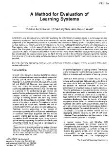
Paths form one of the basic elements of this theory. A path X in Rd is a continuous mapping from some interval [a, b] to Rd , written as X : [a, b] 7→ Rd . We will use the subscript notation Xt = X(t) to denote dependence on the parameter t ∈ [a, b]. For our discussion of the signature, unless otherwise stated, we will always assume that paths are piecewise differentiable (more generally, one may assume that the paths are of bounded variation for which exactly the same classical theory holds). By a smooth path, we mean a path which has derivatives of all orders. Two simple examples of smooth paths in R2 are presented in Fig.1: left panel: right panel:

Xt = {Xt1 , Xt2 } = {t, t3 } , t ∈ [−2, 2]

(1.1)

Xt = {Xt1 , Xt2 } = {cos t, sin t} , t ∈ [0, 2π]

Figure 1: Example of two-dimensional smooth paths. This parametrisation generalizes in d-dimensions (Xt ∈ Rd ) as: n o X : [a, b] 7→ Rd , Xt = Xt1 , Xt2 , Xt3 , ..., Xtd .

(1.2)

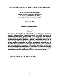
An example of a piecewise linear path is presented in Fig.2: Xt = {Xt1 , Xt2 } = {t, f (t)} , t ∈ [0, 1],

(1.3)

where f is a piecewise linear function on the time domain [0, 1]. One possible example of the function f is a stock price at time t. Such non-smooth paths may represent sequential data or time series, typically consisting of successive measurements made over a time interval.

–2–

Figure 2: Example of non-smooth stochastic path. 1.1.2

Path integrals

We now briefly review the path (or line) integral. The reader may already be familiar with the common definition a path integral against a fixed function f (also called a one-form). Namely, for a one-dimensional path X : [a, b] 7→ R and a function f : R 7→ R, the path integral of X against f is defined by Z b Z b f (Xt ) dXt = f (Xt )X˙ t dt, (1.4) a

a

where the last integral is the usual (Riemann) integral of a continuous bounded function and where we use the “upper-dot” notation for differentiation with respect to a single variable: X˙ t = dXt /dt. In the expression (1.4), note that f (Xt ) is itself a real-valued path defined on [a, b]. In fact, (1.4) is a special case of the Riemann-Stieltjes integral of one path against another. In general, one can integrate any path Y : [a, b] 7→ R against a path X : [a, b] 7→ R. Namely, for a path Y : [a, b] 7→ R, we can define the integral Z b Z b Yt dXt = Yt X˙ t dt. (1.5) a

a

As previously remarked, we recover the usual path integral upon setting Yt = f (Xt ). Example 1. Consider the constant path Yt = 1 for all t ∈ [a, b]. Then the path integral of Y against any path X : [a, b] 7→ R is simply the increment of X: Z b Z b dXt = X˙ t dt = Xb − Xa . (1.6) a

a

Example 2. Consider the path Xt = t for all t ∈ [a, b]. It follows that X˙ t = 1 for all t ∈ [a, b], and so the path integral for any Y : [a, b] 7→ R is the usual Riemann integral of Y: Z b Z b Yt dXt = Yt dt. (1.7) a

a

–3–

Example 3. We present an example involving numerical computations. Consider the two-dimensional path Xt = {Xt1 , Xt2 } = {t2 , t3 }, Then we can compute the path integral Z Z 1 1 2 Xt dXt =

t ∈ [0, 1].

1

t2 3t2 dt =

0

0

3 . 5

(1.8)

(1.9)

The above example is a special case of an iterated integral, which, as discussed in the following section, is central to the definition of the path signature. 1.2 1.2.1

The signature of a path Definition

Having recalled the path integral of one real-valued path against another, we are now ready to define the signature of a path. For a path X : [a, b] 7→ Rd , recall that we denote the coordinate paths by (Xt1 , . . . Xtd ), where each X i : [a, b] 7→ R is a real-valued path. For any single index i ∈ {1, . . . , d}, let us define the quantity Z S(X)ia,t = dXsi = Xti − X0i , (1.10) a