A Priority-Based Preemption Algorithm for Incremental. Scheduling with Cumulative .... To reduce overheads for this on-line scheduling system, two simple ...
A Priority-Based Preemption Algorithm for Incremental Scheduling with Cumulative Resources Qu Zhou and Stephen F. Smith The Robotics Institute Carnegie Mellon University 5000 Forbes Avenue, Pittsburgh, PA 15213 {quzhou,sfs}@cs.cmu.edu
CMU-RI-TR-02-19 July 2002
ABSTRACT When scheduling in dynamic continuous environments, it is necessary to integrate new tasks in a manner that reflects their intrinsic importance while at the same time minimizing solution change. A scheduling strategy that re-computes a schedule from scratch each time a new task arrives will tend to be quite disruptive. Alternative a purely non-disruptive scheduling strategy favors tasks that are already in the schedule over new ones, regardless of respective priorities. In this paper, we consider algorithms that attempt to strike a middle ground. Like a basic non-disruptive strategy, the algorithm we propose emphasizes incremental extension/revision of an existing schedule, rather than regeneration of a new schedule from scratch. However, by allowing selective preemption of currently scheduled tasks, our algorithm also gives attention to the relative importance of new tasks. We consider a specific class of scheduling problems involving the allocation of cumulative (or multi-capacity) resources. We develop an approach to preemption based on the concept of freeing up a resource area (i.e., time and capacity rectangle) comparable to the resource requirement of the new task to be scheduled. Through experimental analysis performed with a previously developed system for air combat operations scheduling, we demonstrate that our priority-based preemption algorithm is capable of producing results comparable in solution quality to those obtained by regenerating a new schedule from scratch with significantly less disruption to the current schedule.
1
1. INTRODUCTION As a scheduling policy, preemption has wide applications in many areas (e.g. CPU scheduling, bandwidth allocation, manufacturing scheduling). Most basically, preemption can be seen as a process that removes (un-schedules, suspends or aborts) one or more previously scheduled activities according to certain criteria and reallocates freed resource capacity to a new activity. A preemption policy is normally used for scheduling high priority activities when a capacity shortage appears. Preemption has been investigated fairly extensively relative to scheduling singlecapacity resources. CPU scheduling, which is central to operating system design, is a representative example, The CPU is single-capacity resource, which can be timeshared to accommodate multiple tasks by algorithms (such as round robin) that repeatedly allocate time slices to competing tasks. Here, a preemptive scheduling policy provides a means for reallocating time slices as new, more important jobs arrive for processing. Preemptive scheduling is much more complex in the context of cumulative or multicapacity resources, and this problem has received much less attention in the literature. The principal complication concerns the selection of which activity (or activities) to preempt. In the case of multi-capacity resources, the number of candidate sets of activities increases exponentially with resource capacity size, while only a single activity must be identified in the single-capacity case. In this paper, we consider the problem of preemptive scheduling of multi-capacity resources. Our broad interest is to define scheduling mechanisms for continuous scheduling environments. By continuous scheduling, we refer to an ongoing planning and execution process, where the scheduler receives new (previously unknown) batches of tasks over time, and these new tasks must be accomplished together with currently executing and previously scheduled tasks. Customer order scheduling and air operations scheduling are examples of continuous scheduling environments. Since, a key concern in such environments is to attempt to minimize change (even when responding to the receive of new, higher priority tasks), we focus on the design of incremental scheduling techniques. Incremental scheduling techniques emphasize revision and extension of an existing schedule rather than periodic regeneration of a new schedule from scratch. We propose an incremental, priority-based preemption algorithm for use in continuous, multi-capacity resource scheduling problems, and evaluate its performance in a complex air campaign scheduling domain where aircraft and munitions capacity must be allocated to various planned air missions. 2. RESEARCH MOTIVATIONS Generally there are two extreme strategies for scheduling in continuous environments as new tasks become known. The first is to simply discard the current schedule, and regenerate a new schedule that incorporates both previously known (but not yet executed) tasks and new tasks. The advantage of this type of strategy is that all tasks can be scheduled at the same time, using the same scheduling criteria. For example, more important tasks (new or old) can always be given priority to receive the best
2
resources and time durations. Its disadvantage is obviously continuing disruption to the existing schedule. The second extreme strategy is to schedule new tasks “on top” of the existing schedule, treating existing resource reservations as additional constraints and allocating only excess available resource capacity to newly received tasks. The benefit of using this strategy is that there is no disruption to the existing schedule. However, some high priority tasks may fail to be scheduled due to the lack of free capacity. The preemption approach proposed here aims at providing some middle ground. By using this approach, a new task can preempt previously scheduled (but lower priority) tasks if there is not enough free capacity to accommodate the new task within its time constraints. At the same time,, by being careful to preempt only those tasks necessary to allow scheduling of new higher priority tasks, the approach attempts to minimise the amount of disruption caused to the current schedule,. Our research work is directly motivated by the problem of air campaign scheduling, which we are addressing within the DARPA “JFACC After Next” (Joint Forces Air Component Commander) research program [Myers and Smith 1999]. The preemption approach is needed to schedule new important tasks (missions) as they arise during an air campaign. Note that although the field of reactive scheduling has proposed many strategies to deal with resource or time conflicts (e.g., [Sadeh et al., 1993, Smith, 1994, El Sakkout et al., 1998 and 2000]), most use a “shifting” strategy to move scheduled tasks in order to reduce resource and temporal contentions caused by scheduling a new task until the schedule consistency is restored. There are obviously limitations of these strategies. •
No matter how important it is, a new task will never be scheduled if the resource capacity is fully allocated and “shifting” fails to completely solve the time/resource conflicts.
•
In reality, unscheduling one task can sometimes be a better solution than disturbing many previously scheduled tasks, though minimal temporal disruption can be achieved by means of certain algorithms [El Sakkout et al., 1998 and 2000].
3. PREVIOUS RESEARCH Bar-Noy et al. [1999] proposed a preemption approach for bandwidth allocation in the design of networks where bandwidth must be reserved for connections in advance. Network bandwidth is a multi-capacity resource. Each task, called a call, requires one or more units of capacity of the network bandwidth for some specific duration. Requests for calls arrive one by one as time proceeds, and all requests must either be serviced immediately or rejected. To reduce overheads for this on-line scheduling system, two simple algorithms were presented. The optimal goal of each is to maximize the throughput of completed calls, where throughput is measured as the sum of the duration times the bandwidth (capacity) requirement.
3
The first algorithm, called left-right (LR) algorithm, implements a compromise between the need to hold on to jobs that have been running for the longest time and the need to hold on to jobs that will run for the longest time in the future. The algorithm gives half of bandwidth capacity to each of these two classes of jobs. In response to the algorithm two sets of calls, L and R, are created. The L set holds a sequence of jobs that are sorted by increasing order of start time. The R set holds a sequence of jobs that are sorted by decreasing order of ending time. A preemption or reject decision will be made to the calls that cannot stay in the sequence of the L or the R because of the sequence’s capacity limit. The second algorithm, called effective time (EFT) algorithm, implements a different compromise, in this case between banking on past profit and ensuring future profit. Rather than dividing the bandwidth between the two classes of jobs, this algorithm attaches a time-value, called the effective time, to each single call. Calls with later effective times are preempted first. The effective time of a call, calli , is equal to the call’s arrival time minus its duration. Effective _ time(call i ) = arrival _ time(call i ) − duration(calli ) The idea behind the simple equation is that the work that has been done is worth twice as much as the work to be done. The comparison of both algorithms shows that the LR algorithm is more effective for calls with small capacity requirement, while EFT is a better choice when calls require large amounts of capacity. One interesting feature of these algorithms is that neither algorithm uses the call’s bandwidth (capacity) requirement as an evaluation criterion. El Sakkout et al. [2000, 1998] combined constraint and linear programming techniques and proposed a unimodular probing backtrack search algorithm for minimizing temporal disruptions in reactive scheduling. This work also considered multi-capacity resources, under the assumption that all tasks require only a single unit of capacity. The constraint programming technique was used to restore schedule consistency, while the linear program was used to minimize temporal disruption from the original schedule. Temporal disruption is measured by the total time shift, i.e. the total change to the start and end times of disrupted tasks. The disruption function is defined to be the sum, over all temporal variables, of absolute time changes. This algorithm can basically be divided into two phases: a resource feasibility phase and a temporal optimisation phase. First, potential resource conflicts caused by scheduling a new task are dealt with by posting the temporal overlays between tasks in the resource feasibility phase. Then, in the temporal optimisation phase, the values of the temporal variable are fixed to values that are consistent and optimal according to the minimal disruption function. Like most of papers on reactive scheduling, a preemption approach is not used in [El Sakkout et al., 1998 and 2000]. Its disruption function is also limited to the sum of temporal variable changes.
4
Ow and Smith et al. [1988, 1995] proposed a set of alternative modification actions for reactive scheduling and corresponding guidelines for action selection. Preemption, also called bumping, was introduced as one of the possible actions. When scheduling a new task, the scheduling search algorithm not only looks for currently free capacity but also considers capacity allocated to lower priority jobs as available capacity. However only single capacity resources and single capacity tasks were considered. To some extent, this paper can be considered as an extension of this work to allow solution of more complicated problems. 4. DESCRIPTION OF THE PROBLEM Aiming at giving a formal description of the preemption problem, this section presents a preemption model that includes four types of representations: resource capacity profile and capacity intervals, scheduled and new operations1, available capacity time blocks and preemption solution. 4.1 Resource capacity profile and capacity intervals Figure 1 shows the capacity profile of a multi-capacity resource r. The total capacity (number of resource units) of the resource is denoted by total _ res _ cap r , which is a positive integer. total _ res _ cap r can usually be divided into two parts: free _ res _ cap r (t ) and alloc _ res _ cap r (t ) . free _ res _ cap r (t ) is the capacity that has not yet been allocated to any operation; alloc _ res _ cap r (t ) represents the capacity that has been allocated to operations. Both of them are functions of time, t. There is a relation between the three capacity representations (see Figure 1).
total _ res _ cap r = free _ res _ cap r (t ) + alloc _ res _ cap r (t ) , where t ≥ 0
free _ res _ cap r ( t )
total _ res _ cap r
alloc _ res _ cap r ( t )
0
intv1
intv 2
intv3
st intv 3
et intv
intv 4
intv5
time
3
Figure 1 Resource capacity profile
1
Operation: operations represent tasks in a schedule. A scheduled task has at least one operation to fullfil the task.
5
The capacity profile of resource r, CPr , consists of a list of capacity intervals. For example, in Figure 1, CPr = {intv1 , intv 2 ,..., intv5 } . Each capacity interval, intvi , is a period of time and has its start and end times, st intvi and et intvi . A given capacity interval is generated when a new operation is scheduled on the resource and the operation’s start or end times are not equal to any capacity interval’s start or end time. In this case an existing capacity interval should be split into two (or three) intervals. Figure 2 shows the generation of a new capacity interval after we schedule a new operation (see Figure 2). new operation
intv1
intv 2
intv 3
intv1
intv 2
intv 3
intv 4
Figure 2 The generation of capacity intervals
It is not difficult to see from Figure 2 that free _ res _ cap r (t ) alloc _ res _ cap r (t ) are constants within every capacity interval. That is
and
∀intvi ∈ CPr : free _ res _ cap r (t1 ) = free _ res _ cap r (t 2 ) , and alloc _ res _ cap r (t1 ) = alloc _ res _ cap r (t 2 ) , where t1 ≠ t2 , stintvi ≤ t1 < etintvi , stintvi ≤ t2 < etintvi . 4.2 Scheduled and new operations
We use Or to represent all scheduled operations on resource r and opi to represent a scheduled operation on resource r. Hence, opi ∈ Or . Let st opi and et opi denote the start and end times of opi , and priorityopi and capacityopi represents opi ’s priority and booked capacity respectively. To represent the resource capacity consumed by opi , we define the resource area, res _ area opi , of opi . It can be computed by the following equation. res _ areaopi = (etopi − stopi ) * capacityopi
6
For the convenience of the following discussion, we also represent the capacity of opi as capopi (t ) , a function of time. capacityop , if st op ≤t < etop i i i capopi (t ) = 0, if t < st or t ≥ et op op i i '
Likely, we use Or to represent a set of new operations that are required to be scheduled on resource r. op k ( opk ∈ Or ) represents a new operation which is required to be scheduled. Similar to opi , priorityopk and capacityop k are used to represent '
op k ’s priority and its required capacity. Let estopk , let opk and d opk denote the earliest
start time, latest end time and time duration of op k respectively. Then we have 0 < d opk ≤ let opk − est opk and res _ areaop k = d op k * capacityop k
4.3 Available capacity time blocks
To schedule a new operation, opk , on resource, r, using normal search mode (i.e., nondisruptively without preemption), we scan the resource’s capacity profile to identify a set of time blocks, TBr with sufficient available capacity. Each time block, tbi ( tbi ∈ TBr ), should cover or partially cover a list of contiguous capacity intervals, {intvmi , intvmi +1 ,...,intvmi + ni } , where mi ≥ 1, ni ≥ 0 . Let sttbi and ettbi denote tbi ’s start and end times, then we have sttbi = max(stintv mi , estop k ) , and ettbi = min(etintv mi + ni , letop k )
The reason for using max and min in the equations is because the first and last intervals ( intvmi and intvmi + ni ) can be partially coved by tbi . Obviously there are both time and capacity constraints on tbi . •
tbi ’s time constraint: ettbi − sttbi ≥ d opk
(1)
7
•
tbi ’s capacity constraint: free _ res _ capr (t ) ≥ capacityop k , where sttbi ≤ t < ettbi
(2)
If no time block can be found because of constraint (2), preemption may be used to obtain additional resource capacity. We refer to this portion of capacity as the required preemption resource capacity, req _ pre _ res _ capr (t ) (see Figure 3). It can be provided by the operations currently scheduled within (or partially within) tbi , which have lower priority than opk has. Let req _ pre _ res _ areatbi denotes the required preemption resource area, then we have : ettbi
req _ pre _ res _ areatbi = ∫ req _ pre _ res _ capr (t )dt . sttbi
free _ res _ cap r (t ) total _ res _ cap r
capacity opk
req _ pre _ res _ cap r (t ) st tbi
et tbi Figure 3 Required preemption area
If we define all lower priority operations covered (or partially covered) by tbi as OPStbi , and, furthermore, define all lower priority operations on resource r as Or , op k , then we have OPStbi = {op j : op j ∈ Or and priorityop j < priorityop k and ( sttbi ≤ stop j < ettbi or sttbi < etop j ≤ ettbi )} Or ,opk =
t OPS
tbi∈TBr
tbi
The new capacity constraint on tbi can be formulated as the follows when preemption is applied:
8
•
tbi ’s capacity constraint in preemption mode:
∑ cap
op j∈OPStbi
op j
(t ) ≥req _ pre _ res _ capr (t ) ≥ capacityopk − free _ res _ capr (t )
where sttbi ≤ t < ettbi
( 2' )
After finding all time blocks based on this constraint, we can certainly preempt all lower operations in (or partially in) any time block to get enough capacity and time duration for opk . However, this can often result in unnecessary disruption, since the resulting resource area that is generated is larger than required. The ideal approach is to select an optimal subset of operations from Or , op k and try to minimize disruptions to the existing schedule. We also call such a subset of operations a preemption solution. The number of preempted operations in the subset, their average priority and total resource area provide three basic criteria for measuring the extent of the disruption to the current schedule. 4.4 Preemption solution
Suppose we can find all subsets of Or , op k , which, together with existing free capacity, can provide both sufficient time duration and capacity to schedule opk . Let S denote all these subsets, S = {S1 , S 2 ,...S n } . Then the preemption solution Sr*, op k ( Sr*, op k ⊆ Or , op k ⊆ Or ) can be theoretically represented as the following. Sr*, op k = min ( w1 ∗ Si + w2 ∗ S i ∈S
∑ priority
op j ∈S i
op j
/ Si + w3 *
∑ res _ area
op j ∈S i
op j
) (3)
As mentioned in the last section, three factors are used in the equation for the selection of Sr*, op k . The first is the number of preempted operations. The second is the average priority of these operations. The last is the sum of resource area of the operations. Different weights ( wi ) can be assigned to the three factors. Note we have made an assumption that the operations in Or cannot be partially preempted. From the above preemption problem description, it can be seen that the crux of the multi-capacity preemption problem is theoretically the optimal selection of a subset of operations Sr*, op k from all lower priority operations Or , op k according to some criteria. It is obviously a combinatorial optimisation problem. In order to get Sr*, op k a search algorithm may search all the subsets of Or , op k , except the empty subset. The size of search space is (2
O r ,opk
− 1) . When Or , op k
is large, searching the space becomes
impractical by using classic search methods (e.g. breadth-first, depth-first and bestfirst). Aiming at avoiding searching the exponential space, the next section proposes two approximate algorithms for efficiently determining a preemption solution ( S r , op k ).
9
5. PREEMPTION ALGORITHM
Two models will be discussed for preemption in this Section. The first model is a simple model in which a new operation does not have estopk and let opk values, but only st opk and etopk . It can be seen as a simplification of the general problem where stopk = estopk , etopk = let opk , d opk = etopk − st opk
Resource allocation problems, in which an operation’s start and end times have been fixed by previous processes, is an example of this model. Machine break down which can be seen as an operation with fixed start time and end time (or time infinity) also belongs to this model. A simple algorithm will be presented for this model in Section 5.1. The second model considers the complete problem, in which estopk and let opk form a time window within which st opk and etopk can be established. An algorithm is also created for this model in Section 5.2. It basically reformulates the model into the first model to which the simple algorithm can be applied. 5.1 Preemption algorithm for operations with fixed start and end times
It is a simplified case to schedule a new operation that has fixed start and end times in the preemption mode. Only one time block can be found on resource r at most, i.e. TBr ≤ 1 . Figure 4 describes the preemption algorithm for the model. Preemption Algorithm1 begin preemption_schedule1(op_id) tb1