IEEE Transactions on Power Delivery, Vol. 12, No. ... network, as a result of variable topologies. .... between the unit and the network impedance from the fault to.
IEEE Transactions on Power Delivery, Vol. 12, No. 2, April 1997
681
A PROBABILISTIC APPROACH TO SETTING DISTANCE RELAYS IN TRANSMISSION NETWORKS
J. Pinto de S6, Senior Member J. Afonso, Student Member Instituto Superior Tknico, DEEC, Sec. Energia, 1096 Lisbon Codex, Portugal
R. Rodrigues E N , Electricidade de Portugal
still further complicates the coordination.
ABSTRACT
The setting of back up zones in distance relays has to deal with fault current infeeds between the relay and remote faults. Traditional approaches to this problem are conservative, some times leaving portions of a Power System without sensitive or selective back up protection. In this paper a probabilistic model for the relay errors resulting from the variation of the infeeds is developed. Other measurement inaccuracies are also considered in order to build a probabilistic approach to setting all zones of distance relays. The developed concepts are associated to automatic tools for computer aided protection coordination and applied to the Portuguese Transmission grid. Keywords: Computer Aided Protection Coordination. 1. INTRODUCTION
The setting process of back up zones in a distance relay has a difficult dilemma when the targeted lines belong to closed loops and dispersed generators are connected to the buses, as in most transmission networks. This dilemma results from the variable distribution of the fault current by the branches of the network, as a result of variable topologies. Changes in a current feeding a fault which are seen by a distance relay do not affect its behavior, with the exception of some extreme situations, such as a SIR too big or CT saturation. This feature is just the major advantage of distance protection regarding the simpler overcurrent relays. The problem arises with currents feeding the fault through nodes (usually buses) between the relay and the fault location, infeeds which are not directly seen by the relay. These infeeds usually have an amplifying effect on the apparent distance. The problem is that, unless this amplifying effect is considered, the actual reach of the relay can be severely reduced and sensitivity missed for remote faults (underreach behavior). On the other hand, if those infeeds are taken into account for setting, the relay can overreach if the infeeds are missing when a remote fault arises. This missing can result from natural changes in the generation profiles or from branch contingencies. In addition, sometimes the infeeds have a reducing effect on the apparent distance (they are actually outfeeds), which
This paper was presented at the 1996 IEEE Transmission and Distribution Conference held in Los Angeles, California, September 15-20, 1996.
The traditional approach to this problem is to take into account no infeed at all [l],which is a simple solution that does not require any fault current computation. However, this solution sacrifices sensitivity and speed for remote back up of most faults for which infeeds are indeed present. Very often this missing sensitivity becomes a selectivity failure when the faults are eliminated by a last back up line of overcurrent relays. This consequence requires the duplication of protection systems in higher voltage levels. But in lower voltage levels of transmission systems, frequently local back up can not be economically justified. This is unfortunate because most hydro plants are connected just to those voltage levels in many networks, as in Portugal. Adaptive relaying schemes [2] will help in solving this drawback, but with present financial constraints many utilities will keep dealing with this classic problem for years to come. With the development of modern computer aids to protection systems analysis, new approaches to coordination have proposed a trade-off between sensitive back-up and selective tripping, by considering a single line contingency (“one-line-out” criterion) [3]. This is suitable for networks with little hydro generation, since the short-circuit current infeeds are then mostly affected by topology changes involving lines only. Such safety consideration assumes that generators are always connected and only one branch may be out for maintenance, fitting the N-1 topology assumed by usual system secure operation. However, for networks with large hydro generation, the distribution of short circuit currents by the branches is very dependent on the generation profiles, because generators of hydro plants are frequently switched on and off. This fact makes the quantification of the effect of the infeeds on the apparent distance a difficult problem. A solution for this problem is presented in the next section. 2. A PROBABILISTIC MODEL FOR THE EFFECT OF THE INFEEDS AND MEASUREMENT ERRORS ON APPARENT FAULT DISTANCES
2.1 - Relationship between infeed variations and generators switching \
Fig. 1 A fault in P to b e reached by a remote back up relay in A and fault current infeeds from other branches. 0885-8977/97/$10.00 0 1996 IEEE
682
To clarify concepts consider Figure 1, in which the sending bus relay of line BC has failed (the relay at the ending bus has opened its circuit breaker since the probability of simultaneous failures in both relays is too small). The apparent impedance for the back up relay at substation A with a remote fault at P is: Zap( A = Z A B + Z B P
(1)
in which R, is the relation between the Ik infeed from another k branch and the current 1 seen by the back up relay:
I
Rk = 'k
The behavior of generators of close plants are better modeled as belonging to the same plant. The parameter b is the ratio between the unit and the network impedance from the fault to the plant. b can be directly estimated through the computation of a new AZ,(A, j, +1) from switching on a second generator (k=2). Simulation experiments confirm the goodness of the quasilinear heuristic, as illustrated in Figure 2. 25
I
-,
(2)
When the generation profile changes, these relations also change. The AZap(A)relative variation of the apparent impedance associated to all the relative variations hR, of the infeeds is:
(3) The dependence of these variations on the changes of the generation profile is first of all a function of the relative lengths of the line segments BP and AP. On the other hand, to determine the range of the variations of the relations A&, a characterization is required for the dependence of those variations on the change of the generation profiles.
To define an efficient way for relating an arbitrary generation profile and the resulting AZap(A),a quasi-linear approach was found to be quite satisfactory. It works as follows:
- For each pair of relays to coordinate, with a fault simulated at the end of the line of the primary relay, Zap@) is first computed for a generation profile with the base generators and a generator per hydro plant switched on. This is an average profile which leads to the best fitting of the quasi-linear approach. Next, a generator is switched off for each j plant and AZap(A,j,-1) is computed through a macro on a suitable software tool [4]. The computation goes on until a sensitivity vector is fulfilled relating each apparent impedance variation with each generator switching state of the system. - The next step is to assume that for an arbitrary generation profile defined by a number of switched on generators, the related AZap(A)can be estimated by a quasi-linear combination of the elementary relationships computed before. A satisfactory solution is usually reached assuming a linear behavior for the currents from different plants (addition of the AZap(A,j) with j belonging to different plants). This approach works well for plants which are not very close. The behavior of generators into the same plant can be modeled as follows: if AZap(A,j,-l) is the apparent impedance variation resulting from switching off a generator, the impedance variation from having k switched on generators in the same plant is given by: (4)
_. Generation Profiles
ig. 2: Illustration of ACP(A) computed through a quasi-linear approach and its true value, for a fault and 10 random generation pro-
files. The sets of the sensitivity and the b vectors relating the variation of the impedance seen by all the back up relays, for their primary relays, and all the generators switching states, can be automatically computed for a complete network using a macro-based programming language running over a commercial software package [5]. For the Portuguese Transmission system this computation takes a few hours of running time on a small old workstation, but these vectors have to be computed only once.
2.2 - Histograms of AZap resulting from the variable infeeds To relate the sensitivity vectors introduced before to the real generation profiles of a Power System, and to weight them by their probability, a report from the last few years of a Control Center can be employed. In Portugal, such a report tracks the generators switching states for each half hour, the last two years having been considered (a dry and a wet year).The Portuguese System has 30 important plants, 25 of which are hydro. Many of these are relatively small plants so that as a whole they generate only from 25 to 50% of the yearly Energy, depending on the weather. However, they have an important role in supplying the peak Power. Quite surprisingly, it was found that the Dispatching had provided almost 18,000 different profiles on a total of 35,040! To take into account so many profiles a statistical approach is the only way. So, in order to achieve a probabilistic description of the infeed consequences, the different profiles were weighted first by their frequency and also by the time-of-the-year fault probability (faults are more frequent by the end of Summer). Next, the AZap were computed for each different profile through the quasi-linear approach described before and weighted accordingly. Even for the 18 thousand different profiles this is a fast operation on an ordinary PC.
683
Line-out contingencies were not considered because of their low probability. As an average each line in these voltage levels (150 and 220 kV in Portugal) has 2 persistent faults per year, the time to repair them not exceeding usually a few hours. Therefore the infeeds variation resulting from such contingencies have an yearly probability around 0,2%, which is not significant comparing to those resulting from the ordinary variation of the generation profiles. Figure 3 shows a typical frequency distribution of the AZap. Most frequency distributions are similar to this, with variations mainly in their parameters. The two relative maximums in the illustrated frequency distribution are typical and can be associated to a base and a peak load set of profiles (the last one is related to the biggest variation). However, sometimes different pattems can be found when 2 or 3 specific plants are important for the infeeds in some region. ~~
~
~
Histogram o f Apparent I m p e d a n c e Variation
The distribution probability of the apparent impedance is thus a random function of z with a density p(Zap(z)) having a range with a maximum and a minimum value, a range proportional to the line length up to its fault. However, the fault location z on a line of length Z, is itself a random variable which can be considered as having an uniform probability density, p(z) = 1 / Z,. Thus, the probability of an apparent impedance Zapis: Zl
P(zaP) =
j PfZaP(Zli+
(5)
0 Fig. 5 shows this p(Zap) probability as it results from integrating the frequency distributions illustrated in Fig. 4 according to (5). It is clear that there is a typical “concentration” of the probable apparent impedances near the sending bus, which however defines their minimum limit.
3.5
................................................................................................................ 3 .o
2.5 h
5
2.0
3n
1.5
.-B ePI
1.0
0.5 0 .o
-11
-4
-6
-9
-I
1
3
8
6
10
13
15
A Z a p (% )
Figure 3: ACP frequency distribution for a fault at the end of a neighboring line as it appears to a back up relay. The variations are around 2& (zZ1) computed for the base generation profile.
It is to point out that these frequency distributions are com-
puted for faults only at the end of each line under back up protection. For any other fault location in the line, the frequency distribution has a simple change in its spreading according to expression (3). Figure 4 illustrates three such frequency distributions for different fault locations in the same line. 0.6
................................................................................................................
1
0.1
* 21
2
= 0.5
II 26
37
48
59
* Zl z=ZI
70
81
92
103
114
125
Apparent Impedance, Zap (51 )
igure 4: Frequency distributions of the Zpimpedances appearing to a back up relay from 3 faults: at the end, at 50% and at 10% of a neighboring line. The line behind has 26 R.
I
26
37
48
59
70
81
QZ
103
114
125
Apparent Impedance, Zap (n)
Fig. 5: Probability density p(Zap) of the apparent impedance of a faulted neighbor line, accounting for the infeed effects. The line behind has 26 n.
2.3 - Probabilistic modeling of measurement errors Besides the random variations of the fault distances appearing to a back up relay, which result from the variable generation profiles, there are also errors in the measurement of those apparent fault distances. These errors are a consequence of the relay own imperfection, CT and VT inaccuracy, and line constants imperfect modeling. A probabilistic model for these inaccuracies was presented in [6], where they were modeled by uniform probability distributions. This is a good working hypothesis, because it overweighs the errors in the extremes and the combination of a number of distributions always yields an approximate gaussian function - particularly good for uniform densities. The range assumed for these errors can be based on typical data, the most important for zone 1 being the inaccuracy of the relay itself, considering fault-induced transients. 5% is a typical catalog error with a confidence level of 95% (IEC 255-3 standard old version), but fault-induced transients dominate for High Speed relays in Europe [7]. A model for zone 1 measurement inaccuracy is therefore a
684
gaussian random variable with zero mean and a standard deviation taken as 8% of the line’s length. Back up zones have the same errors of zone 1 with the exception of fault-induced transients (which are dumped when the relay is delayed), and an increase of the inaccuracy in modeling the line constants of neighbor lines. For non capacitive VT as usual in European lower voltage levels of Transmission Systems, such considerations lead the relay error to a standard deviation around 5.5% for remote faults (4.5% for faults at the ending bus of its own line). These percentages are on the setting values.
frequency distributions. Furthermore, it is now possible for a relay to measure a distance smaller than that of its own line (there is a positive probability for a fault at the sending bus of a neighbor line to be “seen” behind that bus). 3. PROBABILISTIC CRITE IA FOR SETTING
3.1 - Zone 1
20% is the typical margin considered for zone 1 setting in many European countries. For a gaussian probability of error in the measurement of the apparent fault impedance and for lines with two terminals only, such setting provides a conii2.4 - Joint Probability of the measurement errors and of the dence near 99% of not overreaching faults beyond the ending impedance variations resulting from variable infeeds bus. However, it has to be reminded that the relay inaccuracy For a specific fault at location z of a neighbor line, a remote exists both sides of the setting, so that after a relay is set up it back up relay has to deal with an apparent impedance Zap@) can also miss faults behind, its zone 2 being lhen at work, which is a random function of that random location, as explained in 2.2. In addition, for that Zap(z) the measurement The conditional probability of a fault at location z to be seen errors provide a “seen” impedance Zrel= Gel(Zap),as explained into zone 2 of the primary relay (event X) is: in 2.3. Therefore, there are three random variables to account for: the fault location z , the apparent impedance Zap(z),and the measured value Zrel(Zap(z)).
For a given fault location z, the conditional probability density for a back up relay to measure impedance Ze,(z)can be defined by:
3.2 - Zone 2
d z r e l - z a u ( z ),2
while the inconditioned probability density for the relay to measure impedance Zrel is: Zl
1 p(ZreZ(z))Edz
p(Zre1) =
(7)
0 p(Zre1) is illustrated in Fig. 6 for the same line of the previous illustrations. As it is clear from comparing figures 5 and 6, the measurement random inaccuracies have a “filtering” effect n the probability density of Z, computed from the empirical OW
in
0 05
4et,l
where Zset,lis the setting value of the relay zone 1. Zone 2 has two requirements to fulfill: 1) to guarantee the protection of its own line beyond the setting of zone 1, and 2) to provide the maximum fast back up for the neighbor lines starting at the end bus, without superposing zones 2 of their own primary relays. Requirement 1) is mandatory [3] and, for the 43% standard deviation mentioned before, a 99,9% guaranty that its own line is protected requires for the relay zone 2 a setting of at least 1,16 its line length - which can be taken as the lowest limit for setting. Requirement 2) aims at another goal, besides back up: to easy the coordination of zones 3 of the relays behind, allowing their extension while keeping selectivity! For zone 2 of a back up relay to not intersect the zones 2 of its primary relays in the neighbor lines, both the underreach probability of these relays and the overreach probability of the former have to be taken into account. For a zone 2 setting Zset,2of the back up relay (to determine), there is a probability for reaching a fault in z (event Y) which is: Zset ,2
-CO
with p(Zrel(z)) defined by (6) and illustrated in figure 6. Both the densities of p(Xlz) and p(Ylz) arc illustrated in figure 7, with the suitable scales adaptation, 22
36
50
65
79
93
108
Measured Impedance, Zrel(Q)
122
136
151
ig. 6 Probability density p(Zre1) of the relay to “see” fault impec ances, accounting for measurement inaccuracies, random variations of the aparent distances and a uniform density for the fault location on a neighbor line.
Selectivity is missed for a fault at z when both events X and Y arise. These events can be assumed as independent for zone 2. The total probability of missing selectivity for a fault at a neighbor line is: P (X Y) = P (Zre1,z < Z set.2
9
Zrel.1
>Z
set,l>
(10)
685
which can be expressed:
Zset2 ZI
P(x,Y)=
& .f .f p( Zrel,X z ))p( XIz )dzdZrel,2 (1 1)
-m 0 p(Zrel,2(z)) and p(Xlz) are given respectively by (6) and (8). 1.0 0.9
0.8
g
07
F
0.6
k$
0.5
0.4
0.3
Ft
0.2 0.1
0.0 0.02
0.16
0.30
0.44
0.58
0.72
0.86
1.00
Relative Fault Location, z
Figure 7: Probability of a fault at z being seen into both wnes 2 of a primary and of its back up relay with Zset,l and Zset,2 defined for 80% and 67% of the line average apparent impedance, respectively. The finest ascending line shows the missing selectivity probability as a function of z. Its total is 0.93%.
In (10) Zset,2 is the result to obtain, performing numerically the integration while P(X,Y) < E2
(12)
for all the neighbor lines. If the smallest value is chosen, a good value for Ezis 0.1%and it will usually be defined for the shortest line. This will usually mean a missing selectivity probability around 0.1% for the set of all faults in the neighboring, considering all the back up relays. Sometimes the two requirements for setting zone 2 can not be met both. This situation can require an extra coordination time interval (CTI) for zone 2, which can be a problem for loop coordination. However, the experience with the Portuguese network is that such requirement seldom demands an iterative process. This is because such a situation usually arises for short lines under back up, but for those lines the line of the relay under setting, or some other in between, is usually long and there is no need to increase the timing of its zone 2. Therefore only an extra CTI is required for one line in that region and no iteration is usually necessary. For short lines selectivity can also be relaxed to some extent in case of conflicting requirements, the overreach probability being easily computable through (11).However, as a rule the setting of zone 2, computed through the introduced approach, has a much larger reach than the traditional 120% value. 3.3 - Zone 3 Traditionally, zones 3 of distances relays have the goal of providing back up to all the neighbor lines connected to their ending buses [2,3]. To have a full guaranty that this back up is indeed provided, the neighbor line with the maximum appar-
ent distance has to be covered. However, as a rule some of the other neighbor lines are short (as apparent to the back up relay), so that a full back of the longest line means a loss of selectivity for some zones 2 - unless additional CTI are added. It is worthy mentioning that selectivity requirements between zones 3 and 2 may be less constraining than between zones 2 and 1. This is because zones 3 are called to action only when some relay fails and remote back up has to be provided, which is not a frequent event. Anyway, such action will always mean the isolation of a bus of some substation. On the contrary, since most faults are eliminated by zone 1 operations, zones 2 must be higly selective regarding their neighbor lines to avoid spurious tripping. However, a loss of selective back up can lead to the tripping of zones 3 of some relays farther away, making a catastrophic shut down from what could be a severe loss only. Therefore, it was decided for zones 3 to provide the maximum back to the neighbor lines, but without intersecting the zones 3 of their own primary relays with a confidence level of 99%. Because modem distance relays have 4 and even 5 zones, the traditional requirement of full back up was relaxed and left only for the last zone. Zone 3 is taken as only a step further in the back up relaying of neighbor lines. The undertaken approach to setting zone 3 is similar to what was done for zone 2, but now there is a much larger set of computations to do for each back up relay.
As a first step, for the settings values of zones 2 of all its primary relays, corresponding fault locations are determined in each neighbor line, for the base generation profile with the ending circuit-breaker of the neighbor line opened. This location can be done through a fast logarithmic search, applying a macro similar to others presented in the literature [ 5 ] . The next step is the computation of sensitivity vectors relating the variation of the fault distance apparent to the back up relays, with the switching state of a generator per plant. This computation is automatically done only once as it was describe in 2.1 for zone 2. Next, these sensitivities are handled as for zone 2 to reach estimates of the distance variations associated to the real generation profiles, and those estimates are weighted according to the frequency of their profiles. Frequency distributions are achieved this way for each fault associated to each relay pair and to the variable distance apparent to the secondary relay. There were two simplifications in this approach to setting zones 3:
- Correlations between the Mapfor the primary and the secondary relay were neglected. This is a pessimistic assumption, because usually there is a positive correlation between the effect of the infeeds for each relay of a pair.
- It is assumed that the range of the frequency distribution of the Map, computed for a fault at the end of the line of each neighbor’s neighbor, does not change for faults at the beginning of that line (no “compression” is considered). Again, this is a pessimistic assumption, because for shorter
686
lengths their apparent variations are also smaller, as a rule (for zone 3 coordination there are two lines behind the faulted line, hence two buses with random infeeds). 3.4 - Zone 4 For most relays, setting zone 3 to guarantee selectivity as presented in 3.3 does not provide a complete back up to all the neighbor lines. Zone 4 of the secondary relays goes a step further away, with an additional CTI to coordinate with zone 3 of the primary relays. The coordination process for zone 4 can be done similarly to that of zone 3. However, it was found that most often the simpler requirement to provide full back up to all the neighbor lines for a confidence level of 995% also provides selectivity regarding primary zones 3. This full back up (event W in (13)) can be guaranteed choosing the maximum of the Zset,4 computed for faults at the ending points of all the neighbor lines as follows: +m Zl P(W)= p(ZreZ,4(z))dzdZrel,4 < E4 (13) Zl Zset,4 0 where p(Zrel,4(z)) is computed through an expression similar to (6). If this value is lower than the one required for zone 3, the later does not need to be extended. Usually, this Zset,4 value can be set up only for modem relays presenting an operating characteristic capable to avoid load encroachment. CONCLUSIONS
A probabilistic model for the error in distance relays resulting from the variations of the infeeds was presented. Other sources of measurement inaccuracy were also considered to build a probabilistic approach to setting all zones of distance relays. 4th and 5th zones available in modem relays were exploited to reach both sensitivity and selectivity. The developed concepts were embedded in computer tools for protection coordination and applied to the Portuguese Transmission grid. A full description of the developed procedures and of the analysis of their results will be presented soon. ACKNOWLEDGM[ENTS
This work was funded by Electricidade de Portugal (REN) and supported by INTERG, an Institute interfacing Portuguese Universities and Energy-related utilities. REFERENCES 1. The Electricity Council, “Power System Protection vol. III-
Applications”, Peter Peregrinus LTD, New York 1990, pp. 330-334 2. S, S. Venkata, M. J. Damborg, A. K. Jampala and R. Ramaswami, “Computer Aided Protection Coordination”, EPRI Report EL-6145, Dec. 1988, Chapter 7. 3. R. Ramaswami, M. J. Damborg, S. S. Venkata, A. K. Jampala and J. Postforoosh , “Enhanced Algorithms for Transmission Protective Relay Coordination’’, IEEE Transactions on Power Delivery, Vol: PWRD-1, No 1, Jan. 1986, pp. 280-
287, 4. F. L. Alvarado, S. K. Mong and M. K. Enns, “A Fault Program with Macros, Monitors and Direct Compensation in Mutual Groups”, IEEE Transactions on Power Apparatus and Systems, Vol. PAS-104, No 5, May 1985, pp. 11091120.
5. W. English and C. Rogers, “Automating Relay Coordination”, IEEE Computer Applications in Power, July 1994, pp. 22-25. 6. E.R. Sexton and D. Crevier, “A linearisation method for determining the effect of loads, shunts and system uncertainties on line protection with distance relays”, IEEE Transactions on PAS, Vol. 100, N” 11, November 1981, pp. 4434-4441.
7. J.L. Pinto de SA, “Stochastic analysis in the time domain of very high speed digital distance relays, Part 2: Illustrations”, IEE Proc.-Gener. Trans. Distrib., Vol. 141, N”3, May 1994, pp. 169-176. J.L Pinto de S&(1951) is an Associate Professor of lnstituto Superior Tkcnico in Lisbon, Portugal, from where he holds a Ph.D. (1988). His central research interests are in digital relaying, Computer-Aided Protection Engineering and Substations Automation. He published half a dozen papers in the IEEE Transactions.
J. Afonso (1969) is a Master student of Power Systems in lnstituto Superior Tkcnico, now working towards his Thesis. His research theme is in Computer Aided Protection Engineering. He holds a 5year degree in Electrical Engineering and the first prize in the 1995 National Contest which was sponsored by REN for undergraduate work on Power Systems. R. Rodrimes (1957) is the Director of the Protections Department of REN, the Portuguese utility for Power Transmission held by Electricidade de Portugal. He holds a 5-year degree (1980) in Electrical Engineering and a Master in Power Systems (1993) from Instituto Superior Tkcnico.