Journal of Mechanical Science and Technology 24 (12) (2010) 2421~2430 www.springerlink.com/content/1738-494x
DOI 10.1007/s12206-010-0908-0
A probabilistic description scheme for rotating machinery health evaluation† Qiang Miao1,*, Dong Wang1 and Michael Pecht2,3 1
School of Mechanical, Electronic and Industrial Engineering, University of Electronic Science and Technology of China, Chengdu, Sichuan, China 611731 2 Center of Advanced Life Cycle Engineering (CALCE), University of Maryland, College Park, MD 20742 3 Center for Prognostics and System Health Management, City University of Hong Kong (Manuscript Received April 22, 2010; Revised August 9, 2010; Accepted September 1, 2010)
----------------------------------------------------------------------------------------------------------------------------------------------------------------------------------------------------------------------------------------------------------------------------------------------
Abstract Condition-based maintenance has become more popular in recent years because of its advantages in terms of minimizing downtime, extending lifetime, and reducing cost. This kind of maintenance strategy is based on condition monitoring of machinery in operation. Ccondition monitoring is a key step in maintenance decision analysis. Numerous non-stationary signal processing methods have been developed to reveal fault characteristics in rotating machinery. In this study, an adaptive signal analysis method called empirical mode decomposition is employed for gearbox vibration signal preprocessing. Considering a modulation phenomenon that appeared in a faulty gear, the Hilbert Transform is applied to obtain an envelope signature, which usually contains abundant fault-related signatures. Being different from other failure classification problems, this paper is concerned with determining the probability of normal condition based on current observations describing the condition of a gearbox. Moreover, according to Bayes rule, this problem can be translated to estimate the conditional probability of current observations given normal gearbox condition using a Hidden Markov Model. From this point, a novel probabilistic health description index called Average Probability Index is proposed for gearbox health evaluation. For automatic detection, a semi-dynamic threshold is presented to detect an early fault in a gear. At last, validation and comparative studies are performed using two sets of gearbox lifetime accelerated testing vibration data. The results show the advantages of the proposed method for gearbox condition monitoring. Keywords: Condition-based maintenance; Health evaluation; Empirical mode decomposition; Average probability index; Hidden Markov model ----------------------------------------------------------------------------------------------------------------------------------------------------------------------------------------------------------------------------------------------------------------------------------------------
1. Introduction Machinery suffers from many kinds of failures during operation. Thus, research on maintenance becomes necessary to guarantee the reliability of machinery. The history of maintenance engineering can be traced back to run-to-failure maintenance, which does not implement maintenance actions until machinery breakdown. However, this kind of maintenance strategy has many disadvantages, including high downtime, equipment damage, high repair cost, etc. Later, time-based preventive maintenance, which is also called planned maintenance, was developed to perform maintenance activities on the basis of machinery failure statistics. Since it does not consider the current health condition of machinery, time-based preventive maintenance cannot avoid random breakdowns and can even make the total maintenance cost higher. Therefore, it is crucial to explore a new strategy to overcome the aforemen†
This paper was recommended for publication in revised form by Associate Editor Yeon June Kang * Corresponding author. Tel.: +86 28 6183 1669, Fax.: +86 28 6183 0227 E-mail address:
[email protected] © KSME & Springer 2010
tioned disadvantages. Fortunately, a very useful strategy called Condition-based Maintenance (CBM) has been developed to implement a planned maintenance schedule. CBM regards the health condition of machinery as the basis for maintenance decision-making. Therefore, the proper method to monitor the health condition of machinery is a vital question in CBM and is the motivation for this study [1]. Fig. 1 illustrates three main steps in CBM, which can also be treated as three modules: data acquisition, data processing, and maintenance decision-making. First, original signals, such as vibration information, are obtained by using sensors. Second, these signals are processed to extract or reveal fault signatures in order to check the health condition of machinery. Third, effective maintenance policies are planned [1]. Data processing is the key step that extracts critical information from abundant redundancy data collected by the data acquisition module, and the output of it determines the performance of the maintenance decision-making module. Many data processing methods have been developed to reveal fault characteristics of non-stationary mechanical vibration signals. Among all these available methods, the Wavelet
2422
Data acquisition
Q. Miao et al. / Journal of Mechanical Science and Technology 24 (12) (2010) 2421~2430
Date processing
Maintenance decision-making
Fig. 1. A general flow chart of CBM program.
Transform (WT) [2] is widely used in mechanical fault detection. The main advantage of WT is its excellent performance with good time resolution at high frequency and good frequency resolution at low frequency. However, the application of WT has limitations. It is hard to determine which wavelet should be used to measure the similarity between the original signal and the wavelet function and to determine how many decomposition levels are needed. Further, once both wavelet function and decomposition levels are determined, they will be applied to the whole analysis process. That is to say, this method is a non-adaptive signal processing technique. There is also an energy leakage problem owing to the limited length of the wavelet function. In recent years, another novel adaptive time series analysis technique called Empirical Mode Decomposition (EMD) [3] has been developed to analyze non-stationary and non-linear signals. This method is capable of decomposing a signal into a number of Intrinsic Mode Functions (IMFs) according to the local characteristic time/scale of the signal itself. Therefore, the decomposition process is a self-adaptive procedure. What is more, the generated IMFs are stationary. Due to this potential in signal processing, a lot of research has been conducted recently [4-9]. For example, Fan and Zuo [4] employed EMD to decompose raw vibration signals into IMFs, which is a selfadaptive program to detect machine faults at the earliest onset of deterioration. Chen et al. [5] presented an ensemble empirical mode decomposition method in pipeline corrosion inspection. Dong et al. [6] improved the sifting process of EMD for bearing fault diagnosis. Bassiuny et al. [7] employed EMD for fault diagnosis of the stamping process. Gao et al. [8] used EMD to decompose a signal into IMFs and presented the concept of Combined Mode Function (CMF) to solve the failure of IMFs to reveal signal characteristics in case of noise. Li et al. [9] proposed a new Ranged Angle-Empirical Mode Decomposition method to identify the vital components of a diesel engine that have abnormal clearance. Furthermore, the phenomena of signal modulation exist due to the occurrence of local faults in the process of condition monitoring. Since EMD decomposes multi-component amplitude and frequency-modulated signals, and since each obtained IMF may be amplitude-modulated or frequencymodulated, it is necessary to apply the Hilbert Transform (HT) for signal demodulation. With the motivation of emphasizing the capability of EMD in early fault detection, we conducted research to determine EMD’s behavior for online health evaluation of machinery. This is different from the work of others [4-9], as they focused on applying EMD to distinguish different machinery fault patterns, while the goal of our study is to realize online health description with a probabilistic scheme based on EMD and the
Hidden Markov Model (HMM). In this study we extract fault features using a combination of EMD, CMF, and HT. Next, a novel condition monitoring curve, which is described by the Average Probability Index (API), is constructed using HMM due to its success in speech recognition [10]. Moreover, this application of HMM has great novelty because traditional applications of HMM in CBM mostly concentrate on fault diagnosis rather than prognosis [11-13]. Then, a kind of semi-dynamic threshold is defined to detect the occurrence of an early fault. That is to say, an early fault happens when the proposed index API is lower than its corresponding dynamic threshold. The rest of this paper is organized as follows. Section 2 describes a signal processing method using Empirical Mode Decomposition. In Section 3, a novel health evaluation index for a gearbox and its semi-dynamic threshold is proposed. In Section 4, two sets of gearbox vibration data provided by the Applied Research Laboratory at Pennsylvania State University are used to validate the proposed method and comparisons are performed. Conclusions are presented in the end.
2. Signal decomposition scheme 2.1 Empirical mode decomposition The basic idea of Empirical Mode Decomposition is to decompose original signals into different Intrinsic Mode Function (IMF) components. Each IMF must satisfy the following conditions [3]: (1) in the whole data set, the number of extrema and zero-crossings must either equal or differ at most by one. (2) At any point, the mean value of the envelopes defined by local maxima and local minima is zero. An IMF expresses a simple oscillatory mode compared with a simple harmonic function. The decomposition process of any signal x(t ) can be described as follows: (1) Connect all the local maxima of signals using a cubic spline line. The connected line can be called the upper envelope, u1 . (2) Repeat the process for local minima to obtain the lower envelope, l1 . The upper and lower envelopes should cover all of the data between them. (3) The mean of the upper and lower envelopes’ values is m1 , so the first residual h1 can be obtained as follows: u1 + l1 2 h1 = x (t ) − m1 m1 =
(1) (2)
(4) Ideally, if h1 is an IMF, then it is the first component of x(t ) . However, if h1 is not an IMF, it is regarded as the
original signal, and steps (1)- (3) are repeated. That is, h11 = h1 − m11
(3)
Repeat sifting, i.e. up to k times until h1k becomes an IMF, that is,
2423
Amplitude
Q. Miao et al. / Journal of Mechanical Science and Technology 24 (12) (2010) 2421~2430 0.1 0 -0.1
c2
0.1 0 -0.1
c3
10 0 -10
c4
10 0 -10
c5
5 0 -5
c6
2 0 -2
10 0
0.1
0.2
0.3
0.4
0.5
0.6
0.7
0.8
0.9
1
0
0.1
0.2
0.3
0.4
0.5
0.6
0.7
0.8
0.9
1
0
0.1
0.2
0.3
0.4
0.5
0.6
0.7
0.8
0.9
1
0
0.1
0.2
0.3
0.4
0.5
0.6
0.7
0.8
0.9
1
0
0.1
0.2
0.3
0.4
0.5
0.6
0.7
0.8
0.9
1
0
0.1
0.2
0.3
0.4
0.5
0.6
0.7
0.8
0.9
1
Amplitude
c1
0 -5 -10
Fig. 2. EMD decomposition results of x1 (t ) .
h1k = h1( k −1) − m1k .
(4)
Then the obtained IMF can be designated as: c1 = h1k .
(5)
(5) Separate c1 from x(t ) and the residual r1 can be given as r1 = x(t ) − c1 .
(6)
(6) Treat r1 as the original data, and repeat the process as described above n times. As a result, n -IMF of signal x(t ) can be obtained as follows: r1 − c2 = r2
(7) rn −1 − cn = rn .
The decomposition process does not stop until the residual rn becomes a monotonic function or a constant from which
no more IMF components can be extracted. To sum up (6) and (7), we can get: n
∑ c (t ) +r (t ) . i
n
(8)
i −1
2.2 Construction of combined mode function In machinery condition monitoring, a critical problem is the impact of noise, which may be caused by certain systematic factors such as sensor drifting, measurement error, etc. The existence of noise leads to distortion in EMD decomposition. In order to demonstrate this phenomenon, a simulated signal x1 (t ) is defined by adding a noise component. That is, x1 (t ) = 5sin(120π t ) + 7sin(60π t )sin(0.2π t ) + sin(10π t ) + 0.035rand (t ) t ∈ [0,1]
0
0.1
0.2
0.3
0.4
0.5
Time(s) cs
0.6
0.7
0.8
0.9
1
Fig. 3. A CMF cs by combining c3 and c4 .
Time(s)
x (t ) =
5
(9)
where rand (t) is normally distributed white noise. The analy-
sis results of x1 (t ) using EMD are shown in Fig. 2. It is obvious that c4 , c5 and c6 are the major components of x1 (t ) . However, the existence of noise affects the decomposition results and c4 is distorted locally. In order to deal with this problem, the concept of Combined Mode Function (CMF) [8] is applied in this paper. The idea of CMF is to mix neighboring IMFs to obtain a CMF, and this operation increases the accuracy of EMD. Generally, CMF cs is given by: cs = ci + ci +1 +
ci + m
(10)
where 1 ≤ i ≤ n − m, n is the maximal number of IMFs obtained using EMD. In this example, a new CMF, as shown in Fig. 3, is realized by combining c3 and c4 . Through this operation, the distortion caused by noise can be eliminated. 2.3 Demodulation with Hilbert Transform In rotating machinery vibration analysis, another important issue is the impact of signal modulation. For example, in case a tooth failure occurs on a rotating gear, meshing frequency (caused by gear teeth meshing) is modulated by rotating frequency (related to the existence of a fault), which results in the emergence of sidebands around the meshing frequency and its harmonics in spectrum analysis. According to the analysis results in Sections 2.1 and 2.2, each obtained IMF may be amplitude-modulated or frequency-modulated after a multicomponent amplitude-modulated or frequency-modulated signal is decomposed using EMD. Therefore, in order to overcome modulation caused by faults, the Hilbert Transform is employed to reveal fault signatures. For time series x(t ) , its Hilbert Transform, H [ x(t )] , which is a time-domain convolution that maps one real-valued time-history into another, is defined as: H [ x (t )] =
1
π∫
+∞
−∞
x(τ ) dτ . t −τ
(11)
Here, t and τ are the time and translation parameters, respectively. It is known that the Hilbert Transform is a frequencyindependent 90 phase shifter. Thus, this method does not affect the non-stationary characteristics of modulated signals, which may be caused by machine faults. Demodulation can be accomplished by forming a complex-valued time-domain signal called an analytic signal, which is given by
2424
Q. Miao et al. / Journal of Mechanical Science and Technology 24 (12) (2010) 2421~2430
line condition monitoring is usually expected, since it can provide timely information for maintenance decision analysis. In this research, online condition monitoring is realized by collecting vibration data at a certain time interval (e.g., once every 30 minutes) and numbered consequently. Therefore, x j (t ) represents a piece of signal collected at a certain time point j. Assume that the signal x j (t ) collected at time point j is divided into L windows of equal length x1j (t ) , x2j (t ) , …, xLj (t ) . According to the decomposition procedure described in Section 2, L pieces of demodulated CMFs can be obtained and are termed csi' j , i = 1, 2, …, L. The first five steps in Fig. 4 describe this decomposition process, which includes three main tasks: EMD decomposition, construction of CMF, and demodulation with a Hilbert Transform. To extract fault features from demodulated csi' j , spectrum analysis is performed with a Fourier Transform as follows:
Start Load a j th obtained data x j (t ) j
j
j
j
Divide x (t ) into L windows of equal length x1 (t ), x 2 (t ), L , x L (t ) .
IMF components ci1j , cij2 , cij3 ,L, cinj are obtained after applying EMD to
xij (t ), i = 1,2,L L. Employ CMF to obtain c sij , i = 1,2, L L. j
Demodulate c sij , i = 1,2, L L to gain the envelope signals c ' si , i = 1,2, L L .
j
Perform Fourier Transform on c ' si and obtain their absolute values ES sij ( f ) i = 1,2,L L .
Compute the summation of each ES sij ( f ) component and construct input vector T j
Use T 1 to train λ1
ES sij ( f ) =
Probability Evaluation
Use both index API and threshold to monitor the condition of gearbox
End
Fig. 4. The flowchart of the average probability index.
B (t ) = x(t ) + iH [ x(t )] = b(t )eφ (t )
where b(t ) = x 2 (t ) + H 2 [ x(t )] , φ (t ) = arctan
(12) H [ x(t )] , and x(t )
i = −1 ; b(t ) is the envelope of B (t ) .
3. Condition evaluation with health index In order to provide useful information for CBM maintenance decisions, it is necessary to establish a condition monitoring system that can give an actual description of machinery health conditions. Our work described in the previous section mainly focused on signal processing methods, including decomposition of vibration signal with EMD and selection of the appropriate CMF for further analysis. In this section, a novel index called the Average Probability Index is defined on the basis of the selected CMF, which gives a quantitative description of machinery health conditions. The proposed API is constructed using HMM. The key advantage of this method is its adaptiveness, owing to the application of an adaptive signal processing method, EMD, for signal decomposition. Furthermore, to identify the occurrence of an early fault, a semidynamic threshold criterion corresponding to this API index is proposed. In order to better understand the work conducted in this paper, Fig. 4 shows the flowchart of the proposed method. 3.1 Extraction of characteristic features In the implementation of Condition-based Maintenance, on-
∫
+∞
−∞
csi' j (t )e −2π ift dt
i = 1, 2,
L.
(13)
The result of the Fourier Transform reflects the energy distribution of a signal in the frequency domain. In the case of gearbox condition monitoring, the existence of a fault results in a change of energy. Therefore, in the context of gear fault detection, the summation of these amplitude values of the envelope spectrum will increase greatly for a faulty gear compared with a normal gear. Thus, a new term is defined to describe the total energy of csi' j , SES sij = log10 ( sum( ES sij ( f ))) i = 1, 2,
L.
(14)
Finally, a new feature T j can be extracted from the vibration data collected at time j as follows, which includes L feature vectors. T1 j = [ SES sj1 , SES sj2 ,
, SES sLj ]
T2j = [ SES sj2 , SES sj3 ,
, SES sj1 ]
T3j = [ SES sj3 , SES sj4 ,
, SES sj2 ]
TLj = [ SES sLj , SES sj1 ,
, SES sj( L −1) ]
T j = [T1 j , T2j ,…, TLj ].
(15)
(16)
3.2 Definition of API based on HMM When features have been extracted, the proposed health index can be defined using Hidden Markov Model. The HMM is a doubly embedded stochastic model that has been widely applied in pattern recognition, including fault classification. However, the work with HMM in this paper is different from others, since we utilize HMM for the definition of health index rather than fault classification. Generally, an HMM can be represented by a compact notation λ = { A, B, π } . For more details about HMM, the readers is referred to reference [10].
2425
Q. Miao et al. / Journal of Mechanical Science and Technology 24 (12) (2010) 2421~2430
Table 1. Time information of workload change in TR#5. Time period 6/19/97 13:35 Condition #1 (GMT) – 6/23/97 13:35 (GMT) 6/23/97 13:35 Condition #2 (GMT) – 6/24/97 20:56 (GMT)
Time stamp
File number
Workload
000-176
1-12
540 in-lbs (100%max)
192-262
13-83
1620 in-lbs (300%max)
Table 2. Time information of workload change in TR#10. Fig. 5. Mechanical diagnostic test bed.
To define API, assume that the hidden states are governed by a homogeneous Markov chain of order 1. Here, we use T 1 to train HMM λ1 , which represents the normal condition of the gearbox. The purpose of HMM training is to estimate the model parameters λ = { A, B, π } and the training process is realized by fitting the observation probability distribution with Gaussian mixture models (GMMs) for each of the Q states using K-means. After that, improve the parameter estimates of HMM with a mixture of Gaussian outputs using the BaumWelch re-estimation algorithm [10]. Once the HMM for normal conditions is trained, the remaining features, T j s, are used as validation data. Since each feature extracted at time j includes L feature vectors, T j = [T1 j , T2j ,…, TLj ] , we can get a vector of output probability termed as G j = [G1j , G2j ,…, GLj ]. Therefore, a novel index called the Average Probability Index (API) is proposed as follows: API ( j ) =
G1j + G2j + L
+ GLj
j = 1, 2,… n
(17)
Here, variable j corresponds to the time point during vibration data collection. Since the proposed health index is a statistic of probability, we call it a probabilistic scheme for machinery health evaluation. Furthermore, since the lifetime gearbox vibration data used in the case study are collected and numbered sequentially at a certain time interval (e.g., once half an hour) along with the running of the test, time j is consistent with the file number and is represented by the file number (1, 2,…, n) . In order to detect the occurrence of a gear fault, a semidynamic threshold Th(t ) is defined as below, based on the principle of a 3-sigma limit of time series data: t ⎧ ⎪ API (b) ⎪ t t ⎪ b = 1 API (b) ( API (b) − )2 ⎪ t ⎪ b=1 t =1,2,…,tearly , )1/ 2 − 3× ( b=1 ⎪ t t −1 ⎪ Th(t) = ⎨ tearly ⎪ ⎪t API (b) t early ⎪ early t = tearly +1,tearly + 2,…n. b = 1 ⎪ API (b) ( API (b) − )2 ⎪ tearly ⎪ b=1 1/2 b = 1 ) − 3× ( ⎪ t tearly −1 ⎩ early
∑
∑
∑
∑
∑
∑
(18)
Time period 11/17/97 16:20 Condition #1 (GMT) – 11/21/97 16:20 (GMT) 11/21/97 16:20 Condition #2 (GMT) – 11/25/97 13:25 (GMT)
Time stamp
File number
Workload
000-190
1-12
540 in-lbs (100%max)
195-387
13-148
1080 in-lbs (200%max)
Table 3. Gearbox information of TR#5 and TR#10. Gearbox ID#
DS3S0150XX
Make
Dodge APG
Model
R86001
Gear Ratio
1.533
Contact Ratio
2.388
Number of Teeth (Driven gear)
46
Number of Teeth (Driving pinion)
30
Meshing Frequency
875.53 (Hz)
Here, semi-dynamic means that the proposed threshold changes with the historical value of API before the occurrence of an early fault. If the current API is lower than the corresponding threshold at the first time (tearly), we conclude that an incipient fault has occurred. Then, the semi-dynamic threshold becomes a fixed value.
4. Experimental validation 4.1 Experimental setup In this study, two sets of vibration data collected from a mechanical diagnostic test bed (MDTB) (shown in Fig. 5) were used to validate the proposed method. These vibration data were provided by the Applied Research Laboratory at Pennsylvania State University from two test runs of single reduction helical gearboxes, which are named as TR#5 and TR#10, respectively. The experiment started with a brand new gearbox under 100% of the rated workload (Condition #1). After some time, the workload was doubled or tripled (Condition #2), and the test rig was shut down as a result of two accelerometers exceeding a predetermined limit of 150% of the root mean square. There were a series of inspections performed in the process of each test run. Each inspection generates a piece of signal collected in a 10-second window at a sampling rate of
2426
Q. Miao et al. / Journal of Mechanical Science and Technology 24 (12) (2010) 2421~2430
2 0 -2
c3
2 0 -2
c4
0.5 0 -0.5
200
400
600
800
1000
1200
1400
1600
1800
2000
200
400
600
800
1000
1200
1400
1600
1800
2000
200
400
600
800
1000
1200
1400
1600
1800
2000
200
400
600
800
1000
1200
1400
1600
1800
2000
200
400
600
800
1000
1200
1400
1600
1800
2000
c6
0.1 0 -0.1
c7
0.05 0 -0.05
c8
-0.08 -0.09 -0.1
200
400
600
800
1000
1200
1400
1600
1800
2000
200
400
600
800
1000
1200
1400
1600
1800
2000
200
400
600
800
1000
1200
1400
1600
1800
2000
(b)
Amplitude
0.6
2MF
MF
400
4MF
3MF
200 0
500
1000
1500
2000
2500
3000
3500
4000
0.4
FGP1(72)
(a)
20
10 500
1000
1500
2000
2500
3000
3500
4000
15
KI
2MF
MF
400
FGP1(73)
-﹡-: FGP1
0.5
Frequency (Hz)
Amplitude
800 1000 1200 1400 1600 1800 2000
Fig. 8. The signal of CMF and its spectrum with two revolutions. (a) The signal by combining the first four IMFs; (b) its frequency spectrum.
FGP1
MF
20
30
40
50
File number
60
-○-: KI
70
80
KI(72)
10 5
(b) 0
200
(b)
600
Frequency (Hz)
30
0
400
Samplings
Fig. 6. The results of normal gear condition with two revolutions using EMD from TR#5.
0
200
600
Samplings
(a)
0
-2
0.1 0 -0.1
c5
2
(a)
Amplitude
Amplitude
c2
Amplitude
0.5 0 -0.5
c1
KI(71) 20
30
40
50
60
70
80
File number 500
1000
1500
2000
2500
3000
3500
4000
4
Frequency (Hz)
20 kHz. The signal is saved as a data file and numbered sequentially. Tables 1-2 provide the time specifications of TR#5 and TR#10. The mechanical specifications of the gearbox are given in Table 3. 4.2 Signal adaptive decomposition and construction of CMF First of all, API should be emphasized for its adaptive quality because EMD itself possesses an adaptive characteristic in the process of decomposition, compared with Wavelet Transform, Wavelet Packet Transform, and Wavelet Lifting Scheme, which means that there is no need to set the parameters, such as decomposition level, basis function, and so on, to decompose the original signal. To validate the proposed method, we first investigated the performance of the signal decomposition method proposed in this research. Fig. 6 shows the decomposition results of normal gear conditions with two revolutions from TR#5. Through decomposition, 8 IMFs can be obtained, and it is obvious that both c1 and c2 include high frequency components that correspond to the meshing frequency and its harmonics. Fig. 7 demonstrates that the first two components include
API
Fig. 7. Frequency domain exhibition of c1 and c2 with two revolutions. (a) Frequency spectrum of signal c1 ; (b) frequency spectrum of signal c2 .
2 0
API(71) -·-: API --×--: Threshold API(72)
-2
(c)
-4 20
30
40
50
60
70
80
File number
Fig. 9. Comparison of KI, API, and FGP1 using TR#5 under constant torque. (a) Health evaluation using FGP1; (b) health evaluation using KI; (c) health evaluation using API.
the meshing frequency and its harmonics signatures. However, we can also observe that c2 suffers from local distortions between both 600–800 samplings and 1500–1900 samplings. These distortions usually result from noise, and the reasons have been given in the Section 2. On the other hand, we also observe that both c3 and c4 seem to be the losing part of c2 . As a result, in order to mitigate the influence of noise on meshing frequency and its harmonics in later analysis, we combined the first four IMFs into one CMF. Both the time domain signal of CMF and its corresponding frequency spectrum are shown in Fig. 8. 4.3 Evaluation of the proposed Average Probability Index API 4.3.1 Construction of API with constant number of states and GMMs. To begin, we chose a normal data file from TR#5 to repre-
Q. Miao et al. / Journal of Mechanical Science and Technology 24 (12) (2010) 2421~2430 0.8
FGP1
0.7
-﹡-: FGP1
0.6 0.5 0.4
(a)
20
40
60
80
File number
100
120
140
10
-○-: KI KI
5
(b)
0
20
40
60
80 File number
100
120
140
100
120
140
API(39)
0
API
-5
API(40)
-·-: API --×--: Threshold
-10 -15
(c)
20
40
60
80
File number
Further, we used these input features to train the HMM model. The HMM used here is a 5-state model with a diagonal covariance matrix containing a mixture of 3 Gaussian models. Once the HMM of the normal condition is trained, the trained HMM will be used for the whole life of the test with other T j s being the validation data. Finally, we construct API by (17) to reflect the health condition of the gearbox. 4.3.2 Evaluation of API using TR#5 under constant number of states and GMMs. In this section, we will evaluate API and compare it with other fault growth parameters, including FGP1 and KI. FGP1 is defined as the part (percentage of points) of the residual error signal that exceeds three standard deviations calculated from the baseline residual error signal [14]: L
FGP1 = 100
∑ W I (r > r + 3σ ), wi
i
0
(19)
i =1
Fig. 10. Comparison of KI, API, and FGP1 using TR#10 under constant torque. (a) Health evaluation using FGP1; (b) health evaluation using KI; (c) health evaluation using API. Maximum number of GMM
2427
15
where ⎛⎢r − r ⎥ ⎞ wi = I (ri ≤ r + 3σ 0 ) + ⎜ ⎢ i − 1⎥ + 1⎟ I (ri > r + 3σ 0 ) ⎜ ⎢ 3σ 0 ⎥⎦ ⎟⎠ ⎝⎣ L
W=
10
∑w ,
. (20)
i
i =1
5 0
2
3
4 5 State number
6
7
Fig. 11. The relationship between the maximum number of GMMs and state numbers.
sent the gear’s normal status. According to the feature extraction procedure described in Section 3.1, only the first 16 revolution samplings in each piece of the signal were needed to reduce the online computing time. Then, we divided 16 revolution samplings into 8 equal length signals, with L=8. Each of these contained 2118 sampling points, which included 2 revolutions. The decomposition process was introduced in Section 4.2. After we obtained the single CMF, demodulation was needed, and the Hilbert Transform was performed to extract the characteristic signatures. After 8 demodulated CMFs were obtained, we constructed the input features using (13)-(16). The formation of the input features is given as follows: T11 = [ SES s11 , SES s12 ,…, SES s18 ] T21 = [ SES s12 , SES s13 …, SES s11 ] T31 = [ SES s13 , SES s14 ,…, SES s12 ] T81 = [ SES s18 , SES s11 ,…, SES s17 ] T 1 = [T11 , T21 ,…, T81 ].
Here, ri ’s are the current residual error signal points, r is the mean value of the current residual signal, σ 0 is the “baseline” standard deviation, I (⋅) is the indicator function, and ⎢⎣⋅⎥⎦ is the floor function. In addition, another index based on the kurtosis of the residual error signal is presented here for comparison, which is called the Kurtosis Index (KI). The kurtosis usually increases if the signals are properly filtered, and the kurtosis of the residual error signal has been proven to give the earliest indication of gear tooth fault [15]. Then, we used vibration data from TR#5 to evaluate the performance of FGP1, KI, and API for gearbox health evaluation. In TR#5, two adjacent teeth on the drive gear were broken after test-rig shutdown. The total number of running hours was 127.4 hours, including 83 data files. In order to keep a constant workload, we chose data with file numbers from 13 to 83, which corresponded to all vibration data collected under Condition #2. The health evaluation results for the gear fault are shown in Fig. 9. It should be emphasized that the decrease in API represents the deterioration of the machine health condition, while for FGP1 and KI, the increase of the health index represents deterioration. First, we can find that all three indexes can describe the gear health condition. However, the comparison results show that the health trend described by API gradually deteriorates and KI remains almost constant, while the fluctuation of FGP1 is obvious before the occurrence of an early fault. This means that the visual inspection of API and KI is better than FGP1. Since API has its own threshold (red cross marker
2428
Q. Miao et al. / Journal of Mechanical Science and Technology 24 (12) (2010) 2421~2430
line), it can identify the occurrence of early faults automatically. Therefore, we can conclude that API with its semidynamic threshold is the best of the three indexes under constant output torque. 4.3.3 Evaluation of API using TR#10 under constant number of states and GMMs TR#10 was shut down with distributed gear teeth broken on the drive gear at the end of the test. The total number of running hours was 189.25 hours, including 148 data files. Similarly, we chose data files with numbers from 13 to 148. The comparison results are shown in Fig. 10. In Fig. 10, we also see that all three indexes can reflect gear health condition. For FGP1 in Fig. 10(a) it is hard to precisely identify the occurrence of a fault. Moreover, in Fig. 10(b), KI exhibits irregular fluctuation as there is a great change at file number 40 that causes severe distortion for visual inspection. On the other hand, Fig. 10(c) shows that API with its semi-dynamic threshold can detect the occurrence of an early fault in the gear at file number 40. This led us to conclude that API with its semi-
80 60
File number 40 20 0 0
dynamic threshold was the best among the three condition monitoring indexes. 4.3.4 Evaluation of API with different number of states and GMMs It is known that the number of states and GMMs can have an impact on the accuracy of fault diagnosis with HMM. However, in most studies on Hidden Markov Models for fault diagnosis, no detailed discussion is given on how to choose the optimal number of states and GMMs. In order to investigate this problem, an experiment was conducted to vary the number of GMMs under different states based on the work in Section 4.3.2. At the same time, we found that the maximum number of GMMs decreased when the number of states increased. Fig. 11 plots the relationship between the maximum number of GMMs and the number of states in this study. In the following experiments, we fix the number of states at 2 and vary the number of GMMs from 2 to the maximum. Similar to Fig. 9(c), we found that API detected the occurrence of early faults in TR#5 at file number 72 with different GMMs. Further, we varied the number of states from 2 to 7 and repeated the procedure above. Fig. 12 shows the occurrence of an early fault in TR#5 at file number 72. The same experiment was performed in TR#10. The results indicated the occurrence of early faults at file number 40. From Fig. 12 and Fig. 13, we conclude that API has less sensitivity to the selection of number of GMMs and states. In other words, this proposed index can avoid the problem concerning the selection of the optimal number of GMMs and states in the application of HMM with a mixture of Gaussian outputs.
5 10
The number of GMMs
5. Conclusions 15 20
1 3 2 5 4 6 7
The number of states
Fig. 12. The identification of gear fault with different numbers of GMMs and states in TR#5.
40 30
File number 20 10 0 0 5 10
The number of GMMs
15 20
1 3 2 5 4 7 6
The number of states
Fig. 13. The identification of gear fault with different numbers of GMMs and states in TR#10.
In this paper, we developed an adaptive health evaluation index called Average Probability Index (API) based on EMD and HMM. Compared with other research in fault diagnosis with EMD and/or HMM, our purpose was to realize online health evaluation. Therefore, details were given to show the construction of a health index and its threshold criteria. Two sets of vibration data collected from MDTB were used to validate the proposed index with its dynamic threshold. The analysis results showed that API can well describe the health condition of gears. The advantages of this index can be summarized as follows: The proposed index can be regarded as an adaptive one since EMD is an adaptive procedure, compared with Wavelet Transform, Wavelet Packet Transform, and Wavelet Lifting Scheme. API gives a quantitative description of machine health condition, which can be used for estimation of machinery remaining life and maintenance decision analysis. API has less sensitivity to the selection of the number of GMMs and states. The proposed method needs very few samples for model training. Therefore, the dimensionality of data is small, and it
Q. Miao et al. / Journal of Mechanical Science and Technology 24 (12) (2010) 2421~2430
is appropriate for online condition monitoring with less computation time.
Acknowledgment This research was partially supported by National Natural Science Foundation of China (Grant No. 50905028), The Fundamental Research Funds for the Central Universities (Grant No. ZYGX2009X015), and Specialized Research Fund for the Doctoral Program of Higher Education of China (Grant No. 20070614023). We are most grateful to the Applied Research Laboratory at the Pennsylvania State University and the Department of the Navy, Office of the Chief of Naval Research (ONR), for providing the vibration data to develop this work.
References [1] A. K. S. Jardine, D. Lin and D. Banjevic, A review on machinery diagnostics and prognostics implementing conditionbased maintenance, Mechanical System and Signal Processing, 20 (7) (2006) 1483-1510. [2] W. J. Wang and P.D. McFadden, Application of Wavelets to gearbox vibration signals for fault detection, Journal of Sound and Vibration, 192 (5) (1996) 927-939. [3] N. E. Huang, Z. Shen, S. R. Long, et al, The empirical mode decomposition and the Hilbert spectrum for nonlinear and non-stationary time series analysis, Proceedings of the Royal Society of London Series A-Mathematical Physical and Engineering Sciences, 454 (1971) (1998) 903-995. [4] X. Fan, and M. J. Zuo, Machine fault feature extraction based on intrinsic mode functions, Measurement Science and Technology, 19 (4) (2008) 045105. [5] L. Chen, X. Li, X. B. Li and Z. Huang, Signal extraction using ensemble empirical mode decomposition and sparsity in pipeline magnetic flux leakage nondestructive evaluation, Review of Scientific Instruments, 80 (2) (2009) 3082021. [6] H. B. Dong, K. Y. Qi, X. F. Chen, et al., Sifting process of EMD and its application in rolling element bearing fault diagnosis, Journal of Mechanical Science and Technology, 23 (8) (2009) 2000-2007. [7] A. M. Bassiuny, X. Li and R. Du, Fault diagnosis of stamping process based on empirical mode decomposition and learning vector quantization, International Journal of Machine Tools and Manufacture, 47 (15) (2007) 2298-2306. [8] Q. Gao, C. Duan, H. Fan and Q. Meng, Rotating machine fault diagnosis using empirical mode decomposition, Mechanical System and Signal Processing, 22 (5) (2008) 10721081. [9] Y. Li, P.W. Tse, , X. Yang and J. Yang, EMD-based fault diagnosis for abnormal clearance between contacting com-
2429
ponents in a diesel engine, Mechanical System and Signal Processing, 24 (1) 2010 193-210. [10] L. R. Rabiner, A tutorial on hidden Markov models and selected applications in speech recognition, Proceedings of the IEEE, 77 (2) (1989) 257-286. [11] T. Marwala, U. Mahola and F.V. Nelwamondo, Hidden Markov models and Gaussian mixture models for bearing fault detection using fractals, Proceedings of 2006 International Joint Conference on Neural Networks, 3237-3242. [12] H. Ocak and K. A. Loparo, HMM-based fault detection and diagnosis scheme for rolling element bearings, Journal of Vibration and Acoustics-Transactions of the ASME, 127 (4) (2005) 299-306. [13] J. S. Huang and P. J. Zhang, Fault diagnosis for diesel engines based on discrete hidden Markov model, Proceedings of the 2009 Second International Conference on Intelligent Computation Technology and Automation, (2009) 513-516. [14] D. Lin, M. Wiseman, D. Banjevic and A. K. S. Jardine, An approach to signal processing and condition-based maintenance for gearboxes subject to tooth failure, Mechanical Systems and Signal Processing, 18 (5) (2004) 993-1007. [15] A. J. Miller, A New Wavelet Basis for the Decomposition of Gear Motion Error Signals and Its Application to Gearbox Diagnostics, MSc Thesis, The Graduate School, The Pennsylvania State University (1999).
Qiang Miao obtained the B.E. and M.S. degrees from Beijing University of Aeronautics and Astronautics and the Ph.D. from the University of Toronto in 2005. He is currently an Associate Professor and the Chair of the Department of Industrial Engineering, School of Mechanical, Electronic, and Industrial Engineering, University of Electronic Science and Technology of China, Chengdu, Sichuan, China. His current research interests include machinery condition monitoring, maintenance decision-making, and prognostics and health management. Dong Wang received his B.S. and M.S. degrees in Mechanical and Electronic Engineering from University of Electronic Science and Technology of China. He currently is a Research Associate in City University of Hong Kong. His research interests include fault diagnosis, signal analysis and pattern identification.
2430
Q. Miao et al. / Journal of Mechanical Science and Technology 24 (12) (2010) 2421~2430
Michael G. Pecht has a B.S. in Acoustics, an M.S. in Electrical Engineering, and an M.S. and Ph.D. in Engineering Mechanics from the University of Wisconsin at Madison. He is a Professional Engineer, an IEEE Fellow, and an ASME Fellow. He has received the 3M Research Award for electronics packaging, the IEEE Award for chairing key Reliability Standards, and the IMAPS William D. Ashman Memorial Achievement Award for his contributions in electronics reliability analysis. He has written over twenty books on electronic products development, use, and supply chain management. He served as chief editor of the IEEE Transactions on Reliability for eight
years, and on the advisory board of IEEE Spectrum. He has been the chief editor for Microelectronics Reliability for over eleven years, and an associate editor for the IEEE Transactions on Components and Packaging Technology. He is a Chair Professor, and the founder of the Center for Advanced Life Cycle Engineering (CALCE), and the Electronic Products and Systems Consortium at the University of Maryland. He has also been leading a research team in the area of prognostics, and formed the Prognostics and Health Management Consortium at the University of Maryland. He has consulted for over 50 major international electronics companies, providing expertise in strategic planning, design, test, prognostics, IP, and risk assessment of electronic products and systems.