goals of this work are to formally define the concept of situation and to develop a sound probabilistic framework for modeling and recognizing situations. Related ...
A Probabilistic Relational Model for Characterizing Situations in Dynamic Multi-Agent Systems Daniel Meyer-Delius1 , Christian Plagemann1 , Georg von Wichert2 , Wendelin Feiten2 , Gisbert Lawitzky2 , and Wolfram Burgard1 1
2
Department for Computer Science, University of Freiburg {meyerdel,plagem,burgard}@informatik.uni-freiburg.de Information and Communications, Siemens Corporate Technology {georg.wichert,wendelin.feiten,gisbert.lawitzky}@siemens.com
Abstract. Artificial systems with a high degree of autonomy require reliable semantic information about the context they operate in. State interpretation, however, is a difficult task. Interpretations may depend on a history of states and there may be more than one valid interpretation. We propose a model for spatio-temporal situations using hidden Markov models based on relational state descriptions, which are extracted from the estimated state of an underlying dynamic system. Our model covers concurrent situations, scenarios with multiple agents, and situations of varying durations. To evaluate the practical usefulness of our model, we apply it to the concrete task of online traffic analysis.
1 Introduction It is a fundamental ability for an autonomous agent to continuously monitor and understand its internal states as well as the state of the environment. This ability allows the agent to make informed decisions in the future, to avoid risks, and to resolve ambiguities. Consider, for example, a driver assistance application that notifies the driver when a dangerous situation is developing, or a surveillance system at an airport that recognizes suspicious behaviors. Such applications do not only have to be aware of the current state, but also have to be able to interpret it in order to act rationally. State interpretation, however, is not an easy task as one has to also consider the spatio-temporal context, in which the current state is embedded. Intuitively, the agent has to understand the situation that is developing. The goals of this work are to formally define the concept of situation and to develop a sound probabilistic framework for modeling and recognizing situations. Related work includes Anderson et al. (2004) who propose relational Markov models with fully observable states. Fern and Givan (2004) describe
2
Meyer-Delius et al.
an inference technique for sequences of hidden relational states. The hidden states must be inferred from observations. Their approach is based on logical constraints and uncertainties are not handled probabilistically. Kersting et al. (2006) propose logical hidden Markov models where the probabilistic framework of hidden Markov models is integrated with a logical representation of the states. The states of our proposed situation models are represented by conjunctions of logical atoms instead of single atoms and we present a filtering technique based on a relational, non-parametric probabilistic representation of the observations.
2 Framework for Modeling and Recognizing Situations Dynamic and uncertain systems can in general be described using dynamic Baysian networks (DBNs) (Dean and Kanazawa (1989)). DBNs consist of a set of random variables that describe the system at each point in time t. The state of the system at time t is denoted by xt and zt represents the observations. Furthermore, DBNs contain the conditional probability distributions that describe how the random variables are related.
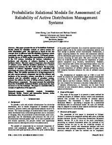
Fig. 1. Overview of the framework. At each time step t, the state xt of the system is estimated from the observations zt . A relational description ot of the estimated state is generated and evaluated against the different situation models λ1 , . . . , λn .
Intuitively, a situation is an interpretation associated to some states of the system. In principle, situations could be represented in such a DBN model by introducing additional latent situation variables and by defining their influence on the rest of the system. Since this would lead to an explosion of network complexity already for moderately sized models, we introduce a relational abstraction layer between the system DBN used for estimating the state of the system, and the situation models used to recognize the situations associated to the state of the system. In this framework, we sequentially estimate the system state xt from the observations zt in the DBN model using the Bayes filtering scheme. In a second step within each time step, we transform the state estimate xt to a relational state description ot , which is then used to
Probabilistic Relational Modeling of Situations
3
recognize instances of the different situation models. Figure 1 visualizes the structure of our proposed framework for situation recognition.
3 Modeling Situations Based on the DBN model of the system outlined in the previous section, a situation can be described as a sequence of states with a meaningful interpretation. Since in general we are dealing with continuous state variables, it would be impractical or even impossible to reason about states, and state sequences directly in that space. Instead, we use an abstract representation of the states, and define situations as sequences of these abstract states. 3.1 Relational State Representation For the abstract representation of the state of the system, relational logic will be used. In relational logic, an atom r(t1 , . . . , tn ) is an n-tuple of terms ti with a relation symbol r. A term can be either a variable R or a constant c. Relations can be defined over the state variables or over features that can be directly extracted from them. Table 1 illustrates possible relations defined over the distance and bearing state variables in a traffic scenario. Table 1. Example distance and bearing relations for a traffic scenario. Relation equal(R, R′ ) close(R, R′ ) medium(R, R′ ) far(R, R′ )
Distances [0 m, 1 m) [1 m, 5 m) [5 m, 15 m) [15 m, ∞)
Relation in front of(R, R′ ) right(R, R′ ) behind(R, R′ ) left(R, R′ )
Bearing angles [315◦ , 45◦ ) [45◦ , 135◦ ) [135◦ , 225◦ ) [225◦ , 315◦ )
An abstract state is a conjunction of logical atoms (see also Cocora et al. (2006)). Consider for example the abstract state q ≡ far(R, R′ ), behind(R, R′ ), which represents all states in which a car is far and behind another car. 3.2 Situation Models Hidden Markov models (HMMs) (Rabiner (1989)) are used to describe the admissible sequences of states that correspond to a given situation. HMMs are temporal probabilistic models for analyzing and modeling sequential data. In our framework we use HMMs whose states correspond to conjunctions of relational atoms, that is, abstract states as described in the previous section. The state transition probabilities of the HMM specify the allowed transitions between these abstract states. In this way, HMMs specify a probability distribution over sequences of abstract states.
4
Meyer-Delius et al.
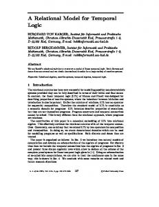
Fig. 2. passing maneuver and corresponding HMM.
To illustrate how HMMs and abstract states can be used to describe situations, consider a passing maneuver like the one depicted in Figure 2. Here, a reference car is passed by a faster car on the left hand side. The maneuver could be coarsely described in three steps: (1) the passing car is behind the reference car, (2) it is left of it, (3) and it is in front. Using, for example, the bearing relations presented in Table 1, an HMM that describes this sequences could have three states, one for each step of the maneuver: q0 = behind(R, R′ ), q1 = left(R, R′ ), and q2 = in front of(R, R′ ). The transition model of this HMM is depicted in Figure 2. It defines the allowed transitions between the states. Observe how the HMM specifies that when in the second state (q1 ), that is, when the passing car is left of the reference car, it can only remain left (q1 ) or move in front of the reference car (q2 ). It is not allowed to move behind it again (q0 ). Such a sequence would not be a valid passing situation according to our description. A situation HMM consists of a tuple λ = (Q, A, π), where Q = {q0 , . . . , qN } represents a finite set of N states, which are in turn abstract states as described in the previous section, A = {aij } is the state transition matrix where each entry aij represents the probability of a transition from state qi to state qj , and π = {πi } is the initial state distribution, where πi represents the probability of state qi being the initial state. Additionally, just as for the DBNs, there is also an observation model. In our case, this observation model is the same for every situation HMM, and will be described in detail in Section 4.1.
4 Recognizing Situations The idea behind our approach to situation recognition is to instantiate at each time step new candidate situation HMMs and to track these over time. A situation HMM can be instantiated if it assigns a positive probability to the current state of the system. Thus, at each time step t, the algorithm keeps track of a set of active situation hypotheses, based on a sequence of relational descriptions. The general algorithm for situation recognition and tracking is as follows. At every time step t,
Probabilistic Relational Modeling of Situations
5
1. Estimate the current state of the system xt (see Section 2). 2. Generate relational representation ot from xt : From the estimated state of the system xt , a conjunction ot of grounded relational atoms with an associated probability is generated (see next section). 3. Update all instantiated situation HMMs according to ot : Bayes filtering is used to update the internal state of the instantiated situation HMMs. 4. Instantiate all non-redundant situation HMMs consistent with ot : Based on ot , all situation HMMs are grounded, that is, the variables in the abstract states of the HMM are replaced by the constant terms present in ot . If a grounded HMM assigns a non-zero probability to the current relational description ot , the situation HMM can be instantiated. However, we must first check that no other situation of the same type and with the same grounding has an overlapping internal state. If this is the case, we keep the oldest instance since it provides a more accurate explanation for the observed sequence. 4.1 Representing Uncertainty at the Relational Level At each time step t, our algorithm estimates the state xt of the system. The estimated state is usually represented through a probability distribution which assigns a probability to each possible hypothesis about the true state. In order to be able to use the situation HMMs to recognize situation instances, we need to represent the estimated state of the system as a grounded abstract state using relational logic. To convert the uncertainties related to the estimated state xt into appropriate uncertainties at the relational level, we assign to each relation the probability mass associated to the interval of the state space that it represents. The resulting distribution is thus a histogram that assigns to each relation a single cumulative probability. Such a histogram can be thought of as a piecewise constant approximation of the continuous density. The relational description ot of the estimated state of the system xt at time t is then a grounded abstract state where each relation has an associated probability. The probability P (ot |qi ) of observing ot while being in a grounded abstract state qi is computed as the product of the matching terms in ot and qi . In this way, the observation probabilities needed to estimate the internal state of the situation HMMs and the likelihood of a given sequence of observations O1:t = (o1 , . . . , ot ) can be computed. 4.2 Situation Model Selection using Bayes Factors The algorithm for recognizing situations keeps track of a set of active situation hypothesis at each time step t. We propose to decide between models at a given time t using Bayes factors for comparing two competing situation HMMs that explain the given observation sequence. Bayes factors (Kass and Raftery (1995)) provide a way of evaluating evidence in favor of a probabilistic model
6
Meyer-Delius et al.
as opposed to another one. The Bayes factor B1,2 for two competing models λ1 and λ2 is computed as B12 =
P (λ1 |Ot1 :t1 +n1 ) P (Ot1 :t1 +n1 |λ1 )P (λ1 ) = , P (λ2 |Ot2 :t2 +n2 ) P (Ot2 :t2 +n2 |λ2 )P (λ2 )
(1)
that is, the ratio between the likelihood of the models being compared given the data. The Bayes factor can be interpreted as evidence provided by the data in favor of a model as opposed to another one (Jeffreys (1961)). In order to use the Bayes factor as evaluation criterion, the observation sequence Ot:t+n which the models in Equation 1 are conditioned on, must be the same for the two models being compared. This is, however, not always the case, since situation can be instantiated at any point in time. To solve this problem we propose a solution used for sequence alignment in bio-informatics (Durbin et al. (1998)) and extend the situation model using a separate world model to account for the missing part of the observation sequence. This world model in our case is defined analogously to the bigram models that are learn from the corpora in the field of natural language processing (Manning and Sch¨ utze (1999)). By using the extended situation model, we can use Bayes factors to evaluate two situation models even if they where instantiated at different points in time.
5 Evaluation Our framework was implemented and tested in a traffic scenario using a simulated 3D environment. TORCS - The Open Racing Car Simulator (Espi´e and Guionneau) was used as simulation environment. The scenario consisted of several autonomous vehicles with simple driving behaviors and one reference vehicle controlled by a human operator. Random noise was added to the pose of the vehicles to simulate uncertainty at the state estimation level. The goal of the experiments is to demonstrate that our framework can be used to model and successfully recognize different situations in dynamic multi-agent environments. Concretely, three different situations relative to a reference car where considered: 1. The passing situation corresponds to the reference car being passed by another car. The passing car approaches the reference car from behind, it passes it on the left, and finally ends up in front of it. 2. The aborted passing situation is similar to the passing situation, but the reference car is never fully overtaken. The passing car approaches the reference car from behind, it slows down before being abeam, and ends up behind it again. 3. The follow situation corresponds to the reference car being followed from behind by another car at a short distance and at the same velocity.
0
600
-200
500
-400
400 bayes factor
log likelihood
Probabilistic Relational Modeling of Situations
-600 -800 -1000 -1200
7
300 200 100 0
passing aborted passing follow
-1400 -1600 5
10
-100 passing vs. follow
-200 15
20 time (s)
25
30
4
6
8
10
12
14
16
18
20
22
time (s)
Fig. 3. (Left) Likelihood of the observation sequence for a passing maneuver according to the different situation models, and (right) Bayes factor in favor of the passing situation model against the other situation models.
The structure and parameters of the corresponding situation HMMs where defined manually. The relations considered for these experiments where defined over the relative distance, position, and velocity of the cars. Figure 3 (left) plots the likelihood of an observation sequence corresponding to a passing maneuver. During this maneuver, the passing car approaches the reference car from behind. Once at close distance, it maintains the distance for a couple of seconds. It then accelerates and passes the reference car on the left to finally end up in front of it. It can be observed in the figure how the algorithm correctly instantiated the different situation HMMs and tracked the different instances during the execution of the maneuver. For example, the passing and aborted passing situations where instantiated simultaneously from the start, since both situation HMMs initially describe the same sequence of observations. The follow situation HMM was instantiated, as expected, at the point where both cars where close enough and their relative velocity was almost zero. Observe too that at this point, the likelihood according to the passing and aborted passing situation HMMs starts to decrease rapidly, since these two models do not expect both cars to drive at the same speed. As the passing vehicle starts changing to the left lane, the HMM for the follow situation stops providing an explanation for the observation sequence and, accordingly, the likelihood starts to decrease rapidly until it becomes almost zero. At this point the instance of the situation is not tracked anymore and is removed from the active situation set. This happens since the follow situation HMM does not expect the vehicle to speed up and change lanes. The Bayes factor in favor of the passing situation model compared against the follow situation model is depicted in Figure 3 (right). A positive Bayes factor value indicates that there is evidence in favor of the passing situation model. Observe that up to the point where the follow situation is actually instantiated the Bayes factor keeps increasing rapidly. At the time where both cars are equally fast, the evidence in favor of the passing situation model starts decreasing until it becomes negative. At this point there is evidence against the passing situation model, that is, there is evidence in favor of
8
Meyer-Delius et al.
the follow situation. Finally, as the passing vehicle starts changing to the left lane the evidence in favor of the passing situation model starts increasing again. Figure 3 (right) shows how Bayes factors can be used to make decisions between competing situation models.
6 Conclusions and Further Work We presented a general framework for modeling and recognizing situations. Our approach uses a relational description of the state space and hidden Markov models to represent situations. An algorithm was presented to recognize and track situations in an online fashion. The Bayes factor was proposed as evaluation criterion between two competing models. Using our framework, many meaningful situations can be modeled. Experiments demonstrate that our framework is capable of tracking multiple situation hypotheses in a dynamic multi-agent environment.
References ANDERSON, C. R. and DOMINGOS, P. and WELD, D. A. (2002): Relational Markov models and their application to adaptive web navigation. Proc. of the International Conference on Knowledge Discovery and Data Mining (KDD). COCORA, A. and KERSTING, K. and PLAGEMANN, C. and BURGARD, W. and DE RAEDT, L. (2006): Learning Relational Navigation Policies. Proc. of the IEEE/RSJ International Conference on Intelligent Robots and Systems (IROS). COLLETT, T. and MACDONALD, B. and GERKEY, B. (2005): Player 2.0: Toward a Practical Robot Programming Framework. In: Proceedings of the Australasian Conference on Robotics and Automation (ACRA 2005). DEAN, T. and KANAZAWA, K. (1989): A Model for Reasoning about Persistence and Causation. Computational Intelligence, 5(3):142-150. DURBIN, R. and EDDY, S. and KROGH, A. and MITCHISON, G. (1998):Biological Sequence Analysis. Cambridge University Press. FERN, A. and GIVAN, R. (2004): Relational sequential inference with reliable observations. Proc. of the International Conference on Machine Learning. JEFFREYS, H. (1961): Theory of Probability (3rd ed.). Oxford University Press. KASS, R. and RAFTERY, E. (1995): Bayes Factors. Journal of the American Statistical Association, 90(430):773-795. KERSTING, K. and DE RAEDT, L. and RAIKO, T. (2006): Logical Hidden Markov Models. Journal of Artificial Intelligence Research. ¨ MANNING, C.D. and SCHUTZE, H. (1999): Foundations of Statistical Natural Language Processing. The MIT Press. RABINER, L. (1989): A tutorial on hidden Markov models and selected applications in speech recognition. Proceedings of the IEEE, 77(2):257–286. ´ E. and GUIONNEAU, C. TORCS - The Open Racing Car Simulator. ESPIE, http://torcs.sourceforge.net