tion, related to the Wishart distribution, for the. Bayes likelihood ..... from a Wishart distribution W 12, 13],. W(Cs p) / jCs ..... 10] J. Glimm and Arthur Ja e. Quantum.
A Probability Model For Errors in the Numerical Solutions of a Partial Di�erential Equation James Glimm Department of Applied Mathematics and Statistics SUNY at Stony Brook, Stony Brook NY 11794-3600 Center for Data Intensive Computing Brookhaven National Laboratory Brookhaven, NY Shuling Hou Theoretical Division, Los Alamos National Laboratory Los Alamos, NM 87545 Hongjoong Kim Department of Applied Mathematics and Statistics SUNY at Stony Brook, Stony Brook NY 11794-3600 David H. Sharp Theoretical Division, Los Alamos National Laboratory Los Alamos, NM 87545 Kenny Ye Department of Applied Mathematics and Statistics SUNY at Stony Brook, Stony Brook NY 11794-3600 Abstract We consider numerical solutions of the Darcy and Buckley-Leverett equations for ow in porous media. These solutions depend on the geology of the porous media, which is given here as a realization of a random eld to describe the reservoir permeability. We measure the solution error as the di�erence between the oil production rates (oil cut) for ne grid and upscaled coarse grid solutions of the equations. The main content of this paper is to formulate and analyze a probability model for this error. On the basis of this error model, we explore the extent to which the coarse grid oil production rate is su�cient to distinguish among geologies or their correlation lengths and to choose correctly the geology (random permeability eld) or its correlation length de ned on a ne grid, and to predict the future oil production rates. We nd that our prediction methodology is e�ective in distinguishing ensembles de ned by di�erent correlation lengths, but that has limited power to distinguish among geologies drawn from a xed ensemble. Our results appear to be weakly sensitive to details in the choice of the error probability model. Our best results are obtained with Bayesian posterior prediction using a nonparametric error model derived from simulation data.
Keywords: Error model, Bayes' prediction, porous media ow
2
1 Introduction The parameter identi cation problem is to determine the coe�cients in a partial di�erential equation given limited observations of the solution. This problem is typically ill posed and its solution is e�ectively non-unique. In an e�ort to recover a well posed, robust solution of the problem, we reformulate it in probabilistic terms: to specify a probability distribution for the equation coe�cients given limited observations. In this formulation, neither the observations nor the solution are known exactly. The errors in each are classi ed by a probability model. Given such a probability error model, and given a prior distribution, Bayes' theorem provides an improved posterior distribution for the coe�cients. The posterior distribution is then used for production forecasts. For the petroleum reservoir problem, the prior distribution comes from a geostatistical model, based upon seismic or outcrop data or other data extrinsic to the uid ow. See [1, 2, 3, 4, 5].
Glimm et al. computational domain. No- ow boundary conditions are imposed on the top and bottom of the cross section. The geology is speci ed by a random permeability eld k(x), x 2 R2 . Typically, k varies by three or more factors of 10. We take k to be a log normal random variable, so that log k is Gaussian and its statistics are completely determined by its mean and covariance matrix. We assume the distribution is stationary, so that the mean is an absolute constant and the covariance is a function of spatial separation only. Each choice of k from the random eld is called a realization. The equations which govern the ow in porous media in their simplest form are v = ?k�rp (Darcy's Law) st + v � rf = 0 (Buckley-Leverett Eqn) r�v =0 (Incompressibility) where v is the seepage velocity, � is a relative total mobility, and p is pressure. s and f represent the saturation and the fractional ux of water, respectively. Gravity, molecular di�usion and capillary pressure are neglected. See [8] for a discussion of these and more general equations. These equations are solved in a rectangle for two dimensional ow. We nondimensionalize the units by specifying the ow domain to be the unit square. The reservoir uids only occupy the pore space between the rocks. In e�ect, all ow takes places within the fraction (porosity � reservoir volume). With this notation we nondimensionalize time by expressing it in units of pore volume of injected
uid (PVI).
The present paper is concentrated with the construction of a probability model for coarse grid solution errors, and an initial exploration of the power of the model in di�erentiating geologies. Also relevant to this study is scale up, or the de nition of the coarse grid equations. These equations are expected to duplicate observed oil production data from a geology speci ed on a ne grid. The coarse grid equations are thus de ned by a ne grid geology, but are solved on a coarse grid through the scale up of permeabilities. We follow the scale up methodology of [6] which provides the reduction in the number of computational degrees of freedom, by a factor of We considered six di�erent permeability en104 in 3D. See also [7]. sembles, de ned by six di�erent x directional correlation lengths �x = 0:25; 0:5; 0:75; 0:85; 0:95; 1:0. In the present study, we consider injection of The correlation length �z in the z direction is water into a petroleum reservoir, and observe the xed at �z = 0:02 and the variance is 2:0. The out ow, through production well(s). The rele- ne grid permeabilities were generated by a movvant out ow variable is the oil-water ow ratio, ing ellipse averaging technique. See [6]. regarded as a time series. The out ow is equal in volume to the in ow since we assume incompressWe study 10 permeability eld realizations ible ow as a simplifying approximation. We re- corresponding to each of three correlation lengths, strict our study to two phase ow (oil and water) �x = 0:25; 0:75; 0:85, and just one realization for for simplicity, and thus ignore production of gas, the other correlation lengths. We assumed that and of the di�erent fractions of petroleum. We each correlation length is equally likely. That consider a 2D cross section with wells at xed is, 6 correlation lengths given to the use in this pressure on the left and on the right sides of the present study each have a prior probability of 61 .
Solution Error Models This probability of 16 is divided by the number of realizations with the same correlation length to give the prior probability for each realization. Thus if we have 10 realizations for one correlation length, each of those 10 realizations has a prior probability of 601 . The permeability eld is speci ed on a 100 � 100 grid. The ow equations above are solved on this same grid. The absolute and relative permeability elds are then coarsened and the equations are solved again to give a coarse grid solution. Several solutions with di�erent degrees of coarseness are obtained. See [6] for further information. In summary, we have the ne grid solution and several coarse grid solutions of the upscaling problem for two phase
ow through a highly heterogeneous two dimensional reservoir cross section. In the context of eld scale, multi-well petroleum reservoir management, we think of geostatistical models of this level of detail as realistic current practice, but the corresponding ne grid simulation could not be performed. Thus in engineering practice, only coarse grid solutions are available. While the ne grid solution is not known in practice, we utilize observations of the solutions (the oil cut) that could be performed on a real reservoir. We denote the model by the symbol m. In the present context, m is uniquely speci ed by the heterogeneous permeability eld k. The log normal distribution for k thus de nes the prior distribution dm. Bayes' theorem states that Ojm)P (m) P (mjO) = R PP((Oj m)P (m)dm Here O is an observation, used to improve the speci cation of the prior probability P (m)dm of the model m. The left hand side, P (mjO), is the posterior probability density, while P (m) on the left is the prior probability density. The likelihood, P (Ojm), is the probability of an observation, given that the model is known to be exactly m. The likelihood is generated by a probability model for solution errors (and in general also for observation errors). Thus we start from the equation Error(t) = Exact(t)?Approximation(t). The main point of this paper is to nd a model stochastic process for the error. This model gives a likelihood for a given error, and serves as a necessary input to Bayes' theorem. This allows de nition of the posterior distribution, based on knowledge of O, which we take here to be the past history of the oil production.
3 We interpret this problem in two ways: (1) If one ne grid solution is considered to be exact, and known but the geology which gives rise to it is not known, to what extent can the geology be selected from an ensemble of geologies and associated known coarse grid solutions, and together with the statistical properties of the error process? (2) Assume that observations of the ne grid solution are known up to time T1 . Using the information up to T1 , can we nd the likelihood for each coarse grid solution and, by Bayes' theorem, the posterior probability predictions of the oil production after T1 ?
2 Probability Models for Numerical Solution Error The error e(t) is a time series. We introduce three measures of the error de ned by this time series. The rst is the L2 norm (L2 ), the second is an Ornstein-Uhlenbeck norm (OU), and the third is nonparametric (NP), de ned by the observed statistics of the solution error. The error model covariance is an operator on a Hilbert space which we want to approximate by a nite matrix. We propose three ways to achieve this goal. By projection into a space of piecewise constant functions (binning), or piecewise linear functions (use of triangle basis elements), or piecewise cubic (cubic splines) functions. Only the rst two of these three possibilities are examined here. Given the error analysis method, there are again a number of choices. We use a maximum likelihood (ML) model, based on the Bayes posterior, and we also use the full posterior pdf for m (Post). We can also represent the likelihood as a simple Gaussian density, based on the observed covariance and its inverse, the precision matrix. This choice is the maximum likelihood estimation of the true covariance, and so gives a ML pdf for the Bayes posterior relative to nite sample size statistics for the NP solution error model. Alternately, we can apply Bayes' theorem to the error model itself, and derive a distribution, related to the Wishart distribution, for the Bayes likelihood. This distribution expresses the likelihood as a weighted integral of Gaussians, and thus is not in itself Gaussian.
4
Glimm et al.
Note that the choice between ML and posterior statistics occurs twice. Once for the geostatistics model to de ne the reservoir, and once for the error model to de ne the likelihood of an observation. In this sense, we apply Bayes' theorem twice. First to the choice of the model (geostatistics) and then to the choice of error model covariance (error model statistics). The present report gives preliminary results which indicate the in uence of some of these choices. A more complete analysis will be published separately.
2.1 Likelihood and Measures for a Time Series A classical random process � (�) de nes � (t) as a random variable for every time t. The Wiener process is an example of a random process. The usual de nition of a random process assumes that it is possible to specify the value � (t) of the process � at every time t. Let H1 be the Schwartz space of rapidly decreasing smooth (test) functions. Actual measurement is accomplished by means of an apparatus which uses some kernel �(t) 2 H1 , Z
� (�) = �(t)� (t)dt; allowing the de nition of a generalized random process. A generalized random process is comparable to a generalized function. The di�erence is that upon integration with a test function, a generalized function results in a real number while the integral of a generalized random process results in a random variable. T Let C be a covariance operator de ned on S = Hj = H1 ; ? 1 < j < 1. C is assumed to
Let L(�) � 1=2(�; C ?1�) for a continuous bilinear form (�). L(�) is called the Lagrangian or the precision or the information operator. It determines the relative likelihood of �. In fact, the Lagrangian is proportional to the negative log of the likelihood. We use a nite dimensional discrete approximation to the in nite dimensional measure as this approximation provides a mathematical basis for the de nition of the in nite dimensional measure. That is, we employ a nite set of parameters to characterize the error. However we cannot approximate the in nite dimensional limit. From the point of view of statistics, too many parameters in the error model would constitute over tting, and would degrade its predictive power. Thus we use the optimum number of degrees of freedom in the error model to adequately represent the information used to de ne it. The nite dimensional approximation is not arbitrarily high in dimension, but is fundamentally limited by the available data (on the numerical solution errors).
3 Stochastic Inversion 3.1 A Conceptual Basis for Inversion For each realization of the permeability eld, the ne grid solution to the Buckley-Leverett equation and Darcy's Law was found. It was assumed to be the exact solution of these equations for this geology. Approximate (upscaled) solutions were found on coarser grids using the RNC method [6].
be continuous and positive de nite as a bilinear form on H1 � H1 . H1 is a nuclear space, a fact which leads to the existenceSof a unique Gaussian measure on its dual S 0 = Hj = H?1 having C as its covariance operator [9]. Let d�C denote this Gaussian measure.
Fine grid solutions from di�erent correlation lengths are shown in Fig. 1 Top. Note a systematic tendency for the oil cut to fall earlier as the correlation length increases. In Fig. 1 Bottom, we show two ne grids for extremes of di�erent correlation length and for each a band of associated coarse grid solutions.
For C = (?�+m2 I )?1 acting on L2 (R1 ) with the identity mapping I and a constant m, d�C is the Ornstein Uhlenbeck measure. C = (?�)?1 de nes Wiener measure and C = I ?1 = I de nes White Noise [10, 9].
A larger horizontal correlation length in the permeability eld typically causes the geology to be dominated by narrow layers. In this case, the oil and the water move rapidly through narrow high conduction channels. The oil saturation
Solution Error Models
5 0.25 0.5 0.75 0.85 0.95 1.0
1.0
Oil Cut
0.8 0.6 0.4 0.2 0.5
1.0 PVI
1.0
0.25 (fine) 0.25 (coarse) 1.0 (fine) 1.0 (coarse)
Oil Cut
0.8 0.6 0.4 0.2 0.5
1.0 PVI
3.2 The Discrepancy De ne a discrepancy as the di�erence between the ne grid solution for one permeability realization and a coarse grid solution for another permeability realization. Our main result is that the discrepancies are systematically larger than the true errors in the case of comparison of realizations of permeability elds having distinct correlation lengths. Thus this bias allows the possibility of distinguishing between di�erent realizations on the basis of the coarse grid solutions alone. For each realization ki of the geology, consider the error ei between the exact (i.e., ne grid) solution fi and the coarse grid solution ci as a random process ei (t) depending on the time variable t. Our purpose is to nd a stochastic process to represent the error function approximately. First let us de ne a weight function (t), de ned as the standard deviation value in the prior measure of the observed error functions, 2 (t) �< (e? < e >)2 >, or more explicitly
Figure 1: Top. Fine grid oil cut vs. PVI for X 2 di�erent correlation lengths. Bottom. Two ne (t) = pi (ei ? �)2 grid solutions and the associated bands of coarse i grid solutions from geologies having distinct cor- where pi is a prior probability for geology i and relation lengths, �x = 0:25 and �x = 1:0. �(t) is the average P of the error ei using the pi as weights �(t) = i pi ei (t).
We use this weight to de ne a normalization
e^(t) of e, curves for the ne grid solutions have steeper slopes after the breakthrough of oil, as seen in Fig. 1 Top. The coarse grid solutions are separated into two distinct bands, for highly distinct correlation length, as seen in Fig. 1 Bottom. The breakthrough time also decreases signi cantly as the correlation length increases. The gure shows clearly that di�erent permeabilities de ne di�erent bands of coarse grid solutions, which mostly do not overlap for a time after breakthrough if the media have su�ciently di�erent statistical properties. This implies that from consideration of the early time coarse grid solution data alone, we have su�cient statistical power to discriminate among geologies having di�erent correlation lengths.
e^(t) � e((tt)) :
We postulate an OU process or White Noise process for the normalized error process of e^(t). For the nonparametric (NP) model, our analysis makes no use of a weight function and so we set e^(t) = e(t) in this case. Note that e= error model requires knowledge of all the ne grid solutions, which is in general not available. But we can assume that those values may be obtained a priori, e.g., by a study such as the one presented here, so we can continue the above procedure without loss of generality. Having started from xed statistical properties of the geology, we next de ne the discrepancy: dij (t) � fi (t) ? cj (t)
6
Glimm et al.
where fi is the ne grid solution for realization i of the geology and cj is a coarse grid solution for realization j . For the L2 and OU analysis, f^ = f= , c^ = c= , and d^ = d= are weighted by the true standard deviation , while for the NP analysis there is no weight and f^ = f; c^ = c; d^ = d. We call d^ij a discrepancy because we think of fi as observed data and cj as a proposed t to this data, based on the geology of the j th realization. e^i = d^ii is the error in the usual sense. In a real oil reservoir, we can observe data f^i but the geology which de nes f^i is not known. One needs a methodology to select a geology which is (able to be) considered as media for f^i and hence the discrepancy. Fig. 2 shows an example of the comparison between the error (i.e., ei (t)) and the discrepancy (i.e., dij (t)). The di�erence in early time should be noted.
Oil Cut
10 error discrepency
5
inverse covariance operator for this process is
C ?1 =
�
�
�
? ddt + m v2 ddt + m
�
(1)
for parameters m and v. The Lagrangian L(d^ij ) from the OU model for d^ij (t) is
L(d^ij ) = v,
Z
v2 ((d^0ij )2 (t) + (md^ij )2 (t))dt
Since the Lagrangian depends on those m and
L(d^ij ) = L(d^ij jm; v);
we need to determine these unknown parameters
m and v. If we know e^i , the Lagrangian becomes L(m; vje^i ). It is reasonable to nd m and v which
maximize L, the negative log likelihood of errors ei . These parameters do not change greatly as the permeability eld is varied.
3.3.2 The White Noise Model If we consider the White Noise process as a model for e^(t), the Lagrangian becomes a multiple of the L2 norm:
0 0.5
1.0 PVI
Z
L(d^ij ) = � d^ij (t)dt 2
Figure 2: Comparison between errors and dis- for a constant �. We put � = 1. crepancies for typical realizations
3.3.3 The Non-Parametric Model
3.3 Models for the Solution Error 3.3.1 The Ornstein-Uhlenbeck Model
Without assuming any postulated model for e^(t) in advance, we can formulate a probability model for the solution error using observed data only. We de ne the precision operator �(t; s) of the error e^(t) as � = C ?1 where C is the true (unobserved) error covariance. � gives the negative log likelihood of the discrepancy. Under a Gaussian assumption, L(d^ij ) = d^ij (t)�d^ij (t)
Di�erent correlation lengths for statistical models yield solutions with a statistically signi cant di�erences in the slope of their oil cut curves, see Fig. 1. Thus the slopes of the discrepancy curves and the area between the discrepancy and the time axis provide possible bases on which to dis- Since C is unknown, C s from sample usually retinguish between discrepancies and errors. The places C . The generation of realizations in our OU process weights both slopes and areas. The current study corresponds to the sampling. This
Solution Error Models
7
choice may be accepted if C s is an unbiased esti- and dispersion can be minimized by selection of mate of C i.e., if a higher order (smooth) subspace and projection operator �p . Thus we expect better results from E(C s ) = C: �1p than from �0p . These ideas are well underfor data smoothing in either applications Using prior probabilities pi , the unbiased esti- stood [11]. mate C s for C is the multiple of the sample covariance,
Cs
= 1? X i
X i
pi
2
!?1
�
pi (ei (t) ? ei (t))(ei (s) ? ei (s)):
3.3.5 The Precision Operator (2)
3.3.4 A Finite Dimensional Approximate Error Covariance Since C s (t; s) is de ned on H1 � H1 , we need to nd a rank p projection Cps (ti ; tj ) of C s (t; s) acting on a p dimensional subspace. A projection operator �p is applied to the errors and discrepancies dij , to yield smoothed discrepancies �p dij lying in a p-dimensional subspace. �p is smoothing in the sense that it suppresses high frequencies. We also de ne Cps = �p C s �p . The problem of choice of the dimension p, and of the approximation space range �p is considered below. If the sample paths e(t) of the error process are smooth, the rate of convergence of the approximation can be improved by choosing �p and its range to be smooth.
We begin with a ML determination of the precision operator �, and represent it as proportional to the inverse of the observed covariance. Due to nite sample errors in the determination of the solution error from numerical experiments, we should consider uctuations of the observed covariance about the true covariance. We let � denote the inverse of the true covariance, so that � is the true precision operator. After projection with the smoothing operator �p , we determine the pdf for the smoothed sample covariance Cps from a Wishart distribution W [12, 13], W (Cps ) / jCps j(n?p?1)=2 j�p jn=2 exp (? 21 Tr�p Cps ): (3)
Here n is the number of observations of the error, and jAj denotes the determinant of A. Since we observe Cps but not �p , we actually want the pdf for �p conditioned on the observation of Cps . The pdf for �?p 1 (the true covariance) is the inverse Wishart distribution IW [12, 13] Let �0p be the operator of projection onto 1 piecewise constant functions, constant over p in- IW (�p?1 jCps ) / jCps jn=2 j�p jn=2 exp (? 2 Tr�p Cps ): tervals of equal length. Applying �0p to the data (4) amounts to binning, that is combining (averaging) all data lying in each subinterval, or bin. Continuing the point of view that we select We also let �1p be the projection onto a p dimensional space of piecewise linear functions. This �p by Bayesian analysis with given data Cps , we space has a basis of triangle shaped hat functions, see that Formula 4 results from Bayes' theorem applied to Formula 3 if a at prior is given for familiar in nite element analysis. the exact covariance �?p 1 . It is customary to divide the error resulting With enough solution error data, n will be from a choice �p 6= I into bias and dispersion. The bias error re ects a shift in the mean val- large, and the optimal p will be large also, so ues and is ameliorated by choosing a large value that the stability of the numerical linear algebra of p. The dispersion has to do with uctuations to nd � from a pdf for �?1 will be an issue. For in Cp , and availability of su�cient data to con- this reason, we prefer the pdf for � directly. This strain Cp , and is diminished by choice of a small is obtained by the multiplication of the IW pdf value of p. Thus p must be selected to possess an by the Jacobian @ �=@ �?1 , where the Jacobian intermediate value. The combined e�ect of bias refers to measures on positive de nite matrices
8
Glimm et al.
only. This Jacobian is known [12], Chap 2 and Hence the posterior oil cut prediction for the ith has the value exact solution f i becomes X j j @ � / j� jp?1 : p w c (t) ? 1 @� j Thus the pdf for �p is given by The normal de nition of ML, namely the L which P (�p jCps ) / maximizes wj , is unsuitable for this problem. Re(5) peated sampling from a single correlation length j�p j n2 ?(p?1) jCps jn=2 exp (? 21 Tr�p Cps ): within the ensemble, as is practiced here to some extent, drives the associated wj to zero, and hence eliminates these geologies from consideration as Formula 5 is still not convenient for applica- the ML geology. Thus we pick the ML geology tion. We write � = TT 0 where T is of lower in two stages. The rst stage is to select the triangular form. The Jacobian @ �p =@Tp is also ML correlation To do this, we sum all known. Thus nally we have a closed form pdf wj with a xed length. � , to get a correlation weight x for the lower triangular square root of �, and the w . The maximum of these de nes the ML cor�x integration space is now a linear space. relation length. Within the geologies having this correlation length, we pick that having the largest The density which results from integration weight wj as the ML geology. over Tp is a mixture of Gaussians, but is no longer Gaussian itself. In the context of the pdf for Tp , we return to the optimal choice of p. A dispersion error corresponds to a highly dispersed pdf for Tp. Thus smoothing does not re ect an error or approximation in the analysis. Rather it re ects a partition 4.1 Prediction of Geology of limited information into the degrees of freedom where it will be most e�ective in reducing Now let us consider a xed realization of the uncertainty. ne grid permeability eld and the corresponding solution fi . Consider the ensemble of all such pairs, with their associated coarse grid solutions. 3.3.6 The ML and Posterior Distribution Given a choice of solution error model or precision matrix, we can nd the Lagrangian values We multiply a likelihood for coarse grid solutions corresponding to the discrepancies. Lagrangian by the prior probability to get a posterior proba- value is the precision operator expectation value. bility. In this way, we de ne a weighted average The Lagrangian value for the exact error between of coarse grid solutions as an approximation to that true ne grid solution and its approximation should usually be smaller than those from the disthe ne grid solution. crepancies using coarse grid solutions from other realizations. We considered the Lagrangian valThe prior possibilities pj and posterior probues up to a time T1 where T1 is the time when abilities wj for j th coarse grid solution cj are dethe oil saturation reaches 60%. In Table 1, we ned by summarize the results for prediction of the geology. The posterior predicted correlation length pj = 6 � 1N (j ) is de ned by the formula.
4 Prediction Results
�
�
wj = Wpj exp ?L(d^ij )
�post = ��jx wj
for discrepancies d^ij where N (j ) is the number of where �jx is the correlation length of geology j . realizations having the same horizontal � correla� The ML correlation length �ML was de ned in P tion length �x and W ?1 = j pj exp ?L(d^ij ) . Sec 3.3.6.
Solution Error Models Geology (Fraction Correct) NP 0.27 OU 0.12 L2 0.21 Prior 0.09
Correlation Relative Relative (Fraction Error Error Correct) (ML) (Post) 0.61 0.10 0.12 0.45 0.22 0.17 0.48 0.21 0.28 0.17
9 the discrepancies with a signi cantly small correlation length become very large. Since very large Lagrangian values imply very small likelihood, the posterior can be thought of as a weighted average of coarse grid solutions from similar correlation lengths only. This is the reason for the improvement.
The relative error in the prediction is by definition
Oil Cut
Table 1: Geology and Correlation Length Predictions. Fraction correct averaged over choice of \exact" geology using the prior distribution
j� ? �i j=�i Post
? �i j=�i
for the ML and posterior predictions respectively. Table 1 lists the fraction of correct predictions for correlation length and the exact geology. These quantities are unstable for prediction, as the number of geologies and correlation lengths in the nite sample from the ensemble increases. Prediction of exact values requires prediction of a set of measure zero. For this reason we focus on relative error statistics. See Table 1. The NP model gives better results, and is e�ective in minimizing the error in prediction of the correlation length.
4.2 Prediction of Future Oil Production Next we predict the future oil productions. If we consider the prior probability as weights for prediction, i.e., if we consider an arithmetic average over correlation length without considering likelihood based on production history observations, that prior approximation gives worse results than those using posterior probabilities. Fig. 3 compares predictions from di�erent Lagrangians. When the di�erences between the correlation lengths are very large, signi cant improvement can be seen in predictions from the posterior probability. The oil production curve (and its band of approximate upscaled solutions) from a large correlation length is noticeably different from that of a small correlation length as Fig. 1 indicates, so that the Lagrangian values for
0.5
PVI
1.0
0.6 Oil Cut
j�
0.4
0.2
ML
and
Fine OU L2 NP Prior
Fine OU L2 NP Prior
0.4 0.2 0.5
PVI
1.0
Figure 3: Comparison of Lagrangians. Fine grid oil cut, L2 , OU, and NP posterior predictions, and prior vs. PVI. Top, �x = 0:25 Bottom, �x = 1:0. We de ne the error reduction for a ML prediction. It is de ned by the di�erence after time T1 between the exact solution and a coarse grid solution having maximum likelihood divided by the prediction error de ned by the prior, i.e., Error reduction from ML = RT i i� T jf (t) ? c (t)jdt P 1RT i j j pj T1 jf (t) ? c (t)jdt where ci� is the highest posterior probability match for the exact solution f i in realization i among the coarse grid solutions cj . Similarly we de ne the error reduction under
10
Glimm et al. OU L2 Post ML Post ML 0.57 0.71 0.56 0.85 0.44 0.55 0.45 0.20 0.79 0.78 1.22 0.88 1.25 1.02 1.32 1.05 0.18 0.18 0.95 0.18 1.03 1.04 1.12 1.04 0.71 0.71 0.94 0.70
0.6
Oil Cut
�x
0.25 0.50 0.75 0.85 0.95 1.00 Mean
NP Post ML 0.60 0.84 0.52 0.51 0.84 0.93 1.11 1.29 0.13 0.10 0.50 0.42 0.62 0.68
0.4
0.2
Table 2: Error reduction with 33 realizations
Error reduction from posterior prediction = RT i T jf (t) ? pp(t)jdt P 1RT i j j pj T1 jf (t) ? c (t)jdt
0.5
PVI
1.0
0.6 Oil Cut
a posterior prediction, i.e.,
Fine NP (ML) NP (Posterior) Prior
Fine NP (ML) NP (Posterior) Prior
0.4
0.2 0.5
PVI
1.0
Figure 4: Comparison of NP maximum likelihood, posterior, and prior predictions to ne where pp(t) is the posterior prediction. grid oil cut vs. PVI. Top, �x = 0:25 Bottom, In Table 2, we see that posterior prediction �x = 1:0. gives better results than the ML or prior prediction. The nonparametric prediction gives the best prediction among alternatives considered here from the given observed data and prior geostatistical probabilities.
These general trends are illustrated in Fig. 4 4.3 E�ects of Data Smoothing which shows that the NP posterior prediction from the posterior probability is better than the prior and essentially identical to the maximum likelihood for two speci c geologies. To study the e�ects of data smoothing on NP prediction, we compare the e�ects of the data The trend in error reduction with respect to smoothing projection operators �0p and �1p for correlation length displayed in Table 2 can be various values of p. We found better results for understood as follows. The prior implies a uni- �1p and we found undersmoothing for values of form weighting of all correlation lengths. Thus it p above about 15. The theoretical formula for will do well for central values of the correlation optimal p depends on a simple (quadratic) oblength and poorly for extremes. Thus the error jective function, such as an L2 norm [11]. Since reduction factor will show the reverse trend being our objective function, future oil production, is smallest at the extremes and larger for the central nonlinearly related to the data (a solution error) values. To further illustrate this fact, we show in being smoothed, we rely on the determination of Fig. 5 the comparison of NP posterior prediction optimal p from computer experiments. The prefto prior and ne grid oil cut for central values of erence of �1p over �0p can be predicted theoretithe correlation length �x = 0:85. We see that for cally from the smoothness of the data, at least central values of correlation length, the prior is for simple objective functions [11]. The results in fact very similar to the NP posterior. are summarized in Table 3.
Solution Error Models
11
6 Acknowledgments
Oil Cut
0.6
0.4
We would like to thank Timothy Wallstrom and Wei Zhu for numerous useful discussions.
Fine NP Prior
The work of JG is supported in part by the NSF Grant DMS-9732876, the Army Research 0.2 O�ce Grant DAAG559810313, the Department of Energy Grants DE-FG02-98ER25363 and DE0.5 1.0 FG02-90ER25084, and Los Alamos National LabPVI oratories under Contract # C738100182X. SH Figure 5: Comparison of oil cut prediction for and DS are supported by the U.S. Department of a central value of horizontal correlation length Energy. HK and KY are supported in part by Los �x = 0:85. NP posterior and prior prediction are Alamos National Laboratories under Contract # C738100182X. compared to the ne grid solution. �1p �0p p 10 15 20 10 15 Post 0.65 0.62 0.71 0.69 0.67 ML 0.64 0.68 0.69 0.66 0.63
20 0.69 0.65
Table 3: Mean error reduction for di�erent data smoothing methods, using the NP error model
5 Conclusion We found three models for the error process between the exact solution and its approximation. All three give improvements in prediction. We prefer the NP model, both because its predictions are better, and also for theoretical reasons, in that it is based totally on data and is formally exact for Gaussian errors. Similarly we prefer the posterior to the maximum likelihood prediction for these two reasons. We prefer rst order data smoothing. We used the solution error model to formulate a conceptual framework for prediction and uncertainty quanti cation, based on a Bayes posterior measure. Applying our results to a porous media
ow problem, we have accuracy within 10% for prediction of the correlation length of the permeability heterogeneity eld, and in error reduction factor of 0.62 (38% reduction) in error for prediction of future oil production.
References [1] C. V. Deusch and A. G. Journel. Geostatistical Software Library and User's Guide. Oxford University Press, Oxford, 1992. [2] H. Haldorsen and L. Lake. A new approach to shale management in eld scale models. In SPE Res. Eng. J., pages 447{452, 1984. [3] A. G. Journel and Ch. J. Huijbregts. Mining Geostatistics. Academic Press, New York, 1978. [4] L. Lake and H. Carroll, editors. Reservoir Characterization. Academic Press, New York, 1986. [5] L. Lake, H. Carroll, and T. Wesson, editors. Reservoir Characterization II. Academic Press, New York, 1991. [6] T. Wallstrom, S. Hou, M. A. Christie, L. J. Durlofsky, and D. H. Sharp. Accurate scale up of two phase ow using renormalization and nonuniform coarsening. Computational Geoscience, 3:69{87, 1999. [7] J. Glimm, H. Kim, D. Sharp, and T. Wallstrom. A stochastic analysis of the scale up problem for ow in porous media. Computational and Applied Mathematics, 17:67{79, 1998. [8] D. Peaceman. Fundamentals of Numerical Reservoir Simulation. Elsevier, Amsterdam{New York, 1977.
12 [9] I. Gelfand and N. Vilenkin. Generalized Functions, Vol IV (English Translation). Academic Press, New York, 1964. [10] J. Glimm and Arthur Ja�e. Quantum Physics: A Functional Integral Point of View. Springer-Verlag, New York, 1981. [11] W. Hardle. Smoothing techniques: with implementation in S. Springer-Verlag, New York, 1991. [12] S. James Press. Applied Multivariate Analysis. Robert E. Krieger Publishing Company, Malabar, Floria, 1982. [13] S. James Press. Bayesian Statistics: Principles, Models, and Applications. John Wiley & Sons, 1989.
Glimm et al.