A Problem Specific Recurrent Neural Network for the Description and Simulation of Dynamic Spring Models Andreas Nürnberger Arne Radetzky Rudolf Kruse University of Magdeburg University of Braunschweig University of Magdeburg Faculty of Computer Science Faculty of Computer Science Faculty of Computer Science 39106 Magdeburg, Germany 38100 Braunschweig 39106 Magdeburg, Germany E-mail: Germany E-mail:
[email protected] E-mail:
[email protected] [email protected] magdeburg.de Abstract In this paper, we present a recurrent neural network which was designed for the description and simulation of dynamic spring models. The network simulates the physical behavior of deformable or elastic solids like stiffness, viscosity and inertia. The physical parameters of the real model can be used to initialize the network parameters. Besides, it is possible to learn the deformation behavior of a real solid. Using a neural network structure, local changes to the system like collisions or cuts can be easily performed during simulation. Furthermore, it is possible to speed up the simulation by parallel hardware.
1. Introduction The simulation of deformable solids is needed in different areas of research. Especially in computer assisted surgery the simulation of elastic tissues is of special importance [1, 3]. In conventional approaches a system of differential equations is constructed by a physical model, e.g. by linear or non-linear spring models [8, 4, 17]. This system can only be solved with heavy computational efforts mostly not in real time, especially when using non-linear spring models. Nevertheless, using finite element models with linear elasticity leads to linear matrix systems, which are easy and fast to solve [1, 4]. However, linear elastic models can only be used for small deformations. A further disadvantage of these approaches is the difficulty to determine the necessary parameters for the springs. The stiffness and viscosity of all springs must be adjusted so that real solids can be convincibly simulated. Mostly this can only be done by extensive testing. To avoid some of these problems we developed an approach based on a recurrent neural network for the
description and simulation of such mesh based models. This approach makes it also possible to apply local changes to the model structure without rebuilding the whole system description as it is necessary in conventional models [1]. Furthermore, by parallel systems the performance of this approach can be significantly enhanced for real time simulation of large objects. The implemented model structure can also be seen as a variation of a cellular automata [15, 16] or a cellular neural network [2]. Since the presented network structure does not fit exactly to one of these model types, only some research results in these areas could be applied to the presented approach. A first prototype implementation of the model was done for the simulation of elastic tissues for the use in computer assisted surgery [14].
2. The used model structure As in traditional approaches for the construction of spring models the mass points of the object are
(a)
(b)
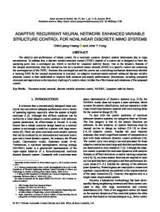
Figure 1: Mass points (nodes) connected with its direct (a) and additionally with its diagonal neighbors (b) via springs
represented as nodes in a 3D mesh (see for example [1]). Thus, the mass of the whole object is divided up between the mass points. We choose this approach because the mesh structure can be easily transferred into a network structure. Furthermore, it is easy to perform cuts in a mesh-based model and existing visualization procedures can be used (for example, texture mapping and volume rendering which are already implemented in hardware.). Every node of the mesh can be connected elastically, rigidly or viscously with its direct or additionally with its diagonal neighbors (see Figure 1). The connections are represented as springs. Most approaches use a mesh that is build without the diagonal springs to speed up the simulation. However, without these springs non-plausible shear effects could occur [8]. The presented model supports both mesh types and it is easy to define different mesh types (even surface meshes) if required. By this, it is possible to speed up the simulation for ‘uncritical’ objects. To every node of the mesh, external forces can be applied (for example gravitation or forces during collision). The internal forces and the displacement of the nodes are computed correspondingly.
3. The network model
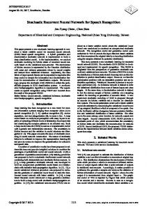
3.1. Mass point dynamic The neurons determining the mass dynamics (inertia) are divided in three ‘sub-neurons’ which calculate the position, velocity and acceleration of the mass point (see Figure 2). An external force can be applied to the neuron, which calculates the actual acceleration. The velocity and position neurons are self-connected feedback nodes. These neurons are used as integrators (see, for example, [5] or [9]). Let tc be the time constant used for simulation, s be the number of springs and NS2 be the connection matrix with ni1 and ni2 be the node numbers connected to spring i, then the neurons can be defined by the following equations. The network input, output and activation functions for all nodes are defined as:
net j =
∑(w
ij
⋅ oi )
i
t c ⋅ net j a j = A j ( net j ) = a j
local propagation
if
next time step
(1)
o j = O j (a j ) = tc ⋅ a j Let k be the number of the node, then the weights are initialized with the following values:
The presented network uses a problem specific structure. The structure of the neural network was designed to speed up the simulation and learning process for elastic solids. In contrast to common neural network models, this model uses vectors instead of single input and output signals. So the standard model of a neuron was vectorized to fit our needs. The structure implements the system of differential equations, which defines the spring model. For this purpose two different network nodes are used. position output
if k = ni1 , 1 acceleration neuron: wij = − 1 otherwise. velocity neuron:
position neuron:
i
velocity output
acceleration
spring forces
Figure 2: Neurons describing the mass point dynamic
1 , m
(2)
wij = 1
These nodes implement the following physical laws which are used for the definition of the physical spring model:
= F = m⋅ a
i
velocity
wij =
where m is the mass of the node.
∑F
position
external forces
if
(acceleration and velocity neuron)
dv =a dt
(velocity neuron)
dp =v dt
(position neuron)
(3)
3.2. Spring dynamic The neurons determining the spring dynamics (see Figure 3) calculate the actual spring force. As in physical
based models the velocity vectors are used to simulate viscosity. The net input and output function for all nodes are defined as: 2
∑(w
ij
⋅ oi )
(4)
spring 4
spring 3
o j = O j (a j ) = a j
a j = A j ( net j ) = SpringFunction( net j ),
(7)
a j = A j ( net j ) = 1 ⋅ net j
These nodes implement the physical laws for spring forces. With equation (3) these forces can be defined as: F = f ( p, v ) + d ( p, v ) ,
node 6
spring 10
spring 11
node 8
spring 12
node 9
(6)
where ViscosityFunction defines the used viscosity function. In case of linear models let c be the spring constant and d be the viscosity constant, otherwise let c = d = 1. Then the force neuron is defined by:
w1 j = c, w2 j = d
spring 7
spring 9
spring 8
node 7
a j = A j ( net j ) = ViscosityFunction( net j ),
node 5
spring 5
(5)
where SpringFunction defines the used spring function (for example, if a linear model is used a linear function which defines the spring forces). The velocity force neuron is defined by:
w1 j = 1, w2 j = −1
spring 6
node 3
1
w1 j = 1, w2 j = −1
node 4
spring 2
1 er lay de no
The activation function and the initial weights of the sub-neurons are defined as follows. The position force neuron is defined by:
node 2
er ay gl rin sp
i =1
spring 1
2 er lay de no
net j =
node 1
(8)
where f(p,v) defines the spring force and d(p,v) the damping force or viscosity. spring force output
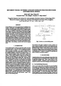
Figure 4: Network representation of a 2D-mesh without diagonal springs
3.3. The network structure A sample of a 2D-mesh is shown in Figure 4. As shown the network is structured by alternating spring and node layers. Of course, different structures can be used to model the objects (see also section 4). The system of differential equations defined by this structure can be derived by equations (3) and (8) (see for example [4, 17]). Modifying the network structure during simulation is easily possible with this model. Performing cuts, for example, can be done by removing springs. Besides, it is possible to simulate ruptures if the spring forces are greater than a threshold value.
3.4. Propagation force
position force
position node 1
position node 2
viscosity
velocity node 1
velocity node 2
Figure 3: Neurons describing the spring dynamic
The used propagation algorithm is separated in two steps. During the first step (local propagation) the network is propagated until a local energy minimum is reached (the nodes of the mass points in the network reached its positions for the current time step). This is similar to the propagation in Hopfield networks [6]. During this propagation step the activities of the mass neurons are not modified (see equation (1)). The second step (next time step) is used to calculate the activities ai of the sub-neurons for the next time step
(equation (1)). At the end of this propagation step the activity of the node sub-neurons defines the position, velocity and acceleration of the mass points at time t0 + n⋅tc, with n be the number of the actual propagation step. In both propagation steps the net is frozen in its current state at the beginning of each propagation step. Then all spring layers are calculated (see Figure 3). The inputs of the spring layers are the position and velocity vectors of the nodes connected with the springs. The output of each spring is a force vector in the direction of the spring. If all springs are updated the propagation of the node layer is started. As net input of each node the weighted sum of the external and internal force vectors is used (see Figure 2). The internal force vectors are received from the connected spring nodes. Under consideration of the node’s mass, the acceleration-neuron computes the node’s acceleration, which is used as input of the velocity neuron. The selffeedback at the velocity and position neurons performs a time-dependent integration. The dynamic behavior is realized with the additional feedback over the springs (see Figure 3). The computation can be done parallel with all nodes and springs. To compute this network it is effective to group several nodes and springs to greater units and solve each unit on a single processor. The order of computation of the node and spring layers during propagation is important to minimize the required propagation steps. Therefore, a heuristic is used to determine the starting node of each propagation. During the first propagation, the node with the greatest force vector is identified. Then the next propagation starts with this node and continuously goes on layer by layer until all nodes are computed. During the propagation, the node with the greatest force difference between the old force and the new computed force is identified. If the force difference is greater than a threshold value, the propagation starts over. The network converges to the fixed point defined by the energy minimum of the dynamic system if it exists. For example, the exterior points of the mesh are fixed and a constant force is applied to one node. A periodical oscillation can occur, for example, in case of object rotation. If the parameters of the network are badly defined (e.g. small spring constants, zero viscosity) the network tends to an unstable (chaotic) behavior. During propagation the network is updated using the time constant tc. In real time applications this constant can be used to define the graphic refresh rate. Thus, it is possible to synchronize the propagation process with a real time environment (see, for example, the third application example in section 4).
3.5. The learning methods The learning methods we are currently working on are based on backpropagation learning methods for recurrent neural networks (see, for example, [5, 9, 11, 12, 18]). The learning algorithms use measured data or data generated by an exact physical model of the tissue for learning. The learning algorithms use the position of every node at discrete time-steps as input. The learning algorithm tries to minimize the error (total cost) function of the network, which is defined as: T T 1 E = ∑ E( t ) = ∑ ∑ ( Ek ( t ))2 t =0 t =0 2 k
Let t = 0, 1, ..., T be the time-step, yk(t) the position of node k and pk(t) the position of the node k in the exact physical model at the time-step t, then Ek(t) is defined as
p ( t ) − y ( t ) if node k has a desired k k output p k at time t, Ek ( t ) = 0 otherwise. The parameters (weights) of the network are adapted after each time-step by a gradient descent method. The learning process is finished if E is sufficient small. In this way, even local differences in the solid structure can be learned. During learning only the weights of the velocity subneurons (the masses mj) and the spring neurons are modified to ensure the interpretability of the network. Although, we are improving these learning approaches, the first results are very promising. We are confident to be able to present further results in the very near future. Another approach to initialize the weights of the network is to use a fuzzy system [7, 10]. The fuzzy system can be used to describe the relations between existing (vague) expert knowledge of the solid behavior (for example ‘very hard’, ‘soft’, ‘elastic’) and the network parameters [13].
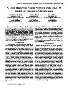
4. Application Examples In this part, we present some examples of applications of our model. The used simulation programs were written in C++ using OpenGL or Open Inventor. The simulation model used in the first example was constructed by 64 nodes and 252 springs. The model was computed on a Pentium 200 PC with at least 20 frames per second. It shows a cube shaped solid under the influence of gravity (see Figure 5).
t = 0.5 s
t=2s
t=4s
t = 22.5 s
t=0s
t=5s
Figure 5: A solid under influence of gravity
A gravity force vector is applied to every node. After less then one second, the cube hits the ground and is deformed at t = 2 s. The collision is detected by a simple plane cross check. If a node crosses the plane, its position is fixed until a reverse force occurs. In this example, the viscosity of the springs is ‘very high’ so that the cube does not bounce off the ground. The deformation reaches its maximum at about t = 4 s. After that, the cube begins to rebuild its initial shape. At time t = 22.5 s the network has nearly a neutral position. The cube did not obtain its old appearance due to the remaining gravity. The next example, presented in Figure 6, shows the simulation of a filled gall bladder. The network is irregular structured and consists of 170 nodes and 396 springs. The simulation was done in real time with 10 frames per second on a dual Pentium 200 PC. One processor was used for visualization and the other for the propagation of the network. Two forces were applied to exterior nodes of the mesh for 5 sec. (as depicted by lines in Figure 6 during time steps t = 0 sec. to t = 5 sec.). The left end of the net was fixed. When the external forces where removed (t = 6 sec.) the gall bladder starts to wobble as expected until it reaches a nearly neutral position (t = 16 sec.). In Figure 7 an example of virtual laparoscopy is presented. The Fallopian tube, which is manipulated by laparoscopic devices, is simulated by an implementation of the presented model on a Silicon Graphics Onyx2 Infinite Reality [14]. The simulation model of the Fallopian tube is build by use of 160 nodes and 610 springs. The other organs are modeled conventionally. On an Onyx2 the simulation can be done with 40 frames per second using only one processor.
t=6s
t = 16 s Figure 6: Simulation of a gall bladder
Figure 7: Example of virtual laparoscopy
5. Conclusion and future work In section 4 we have shown, that the developed model can be used successfully for the simulation of deformable objects. Even on low-cost hardware (for example Pentium PC’s) it is possible to simulate small objects appropriately. Since the presented propagation algorithm can be modified easily to be executed on multiprocessor systems, even larger objects can be simulated on standard hardware. Because of the local propagation during simulation, it is easy to apply external forces to any node, for example gravity forces or collision forces caused by medical tools. Furthermore, changes of the object’s structure can be done during simulation, for example changes caused by cuts, ruptures or fractions. The weights of the network can be initialized by real mass and spring parameters. Besides these parameters can be adapted or learned by use of a physical model or measured data of real objects. Nevertheless, the propagation procedure has to be analyzed in more detail, to be able to evaluate the quality and stability of the propagation process. For example, the stability could perhaps be improved by slowly rising or adapting the time constant during local propagation. Besides, we are currently working on improvements for the learning procedure. At present we are only able to learn the behavior of simple deformable solids. Actual information concerning this project can be obtained via the internet from http://fuzzy.cs.unimagdeburg.de/∼nuernb or http://www.umi.cs.tubs.de/arne.
6. References [1]
[2]
[3]
Bro-Nielsen, M., Surgery Simulation Using Fast Finite Elements. In Visualization in Biomedical Computing, Vol. 1131 of Lecture Notes in Computer Science. Springer, Berlin, Heidelberg et al., 1996, pp. 529-534. Chua, O. and Yang, L., Cellular Neural Networks: Theory, Cellular Neural Networks: Applications, IEEE Trans. Circuits Syst., vol. 35, 1257-90, Oct. 1988 Cotin, S.; Delingette, H.; Ayache, N., Real Time Volumetric Deformable Models for Surgery Simulation. In Visualization in Biomedical Computing, Vol. 1131 of Lecture Notes in Computer Science. Springer, Berlin, Heidelberg et al., 1996, pp. 535-540.
[4]
Gould, P. L., Introduction to Linear Elasticity, Springer, New York, 1994
[5]
Hayken, S., Neural Networks, Prentice-Hall Inc., New Jersey, London, et. al., 1994
[6]
Hopfield, J. J., Neural networks and physical systems with emergent collective computational abilities. Proc. Nat. Acad. Sci., pages 79:2554-2558, USA, 1982
[7]
Kruse, R.; Gebhardt, J.; Klawonn, F., Foundations of Fuzzy Systems. John Wiley & Sons, Inc. , New York, Chichester, et.al., 1994
[8]
Kuhn, Ch., Modellbildung und Echtzeitsimulation deformierbarer Objekte zur Entwicklung einer interaktiven Trainingsumgebung für die Minimal-invasive Chirurgie, PhD Thesis, FZKA 5872, Forschungszentrum Karlsruhe, Germany, 1997
[9]
Lin, Chin Teng and Lee, C. S. George, Neural Fuzzy Systems: A Neuro-Fuzzy Synergism to Intelligent Systems. Prentice-Hall Inc., New Jersey, London, et. al., 1996
[10] Nauck, D., Klawonn, F., and Kruse, R., Foundations of Neuro-Fuzzy Systems, John Wiley & Sons, Inc., New York, Chichester, et.al., 1997 [11] Pineda, F.J., 1987, Generalization of back-propagation to recurrent neural networks, Physical Review Letters, 59(19):2229-2232 [12] Pineda, F.J., 1989, Recurrent back-propagation and the dynamical approach to adaptive neural computation, Neural Computation 1:161-172 [13] Radetzky, A., Nürnberger, A., Pretschner, D. P., A NeuroFuzzy Approach for the Description and Simulation of Elastic Tissues, In Proc. of the European Workshop on Multimedia Technology in Medical Training, Aachen, Germany, 1997 [14] Radetzky, A., Nürnberger, A., Pretschner, D. P., The Simulation of Elastic Tissues in Virtual Medicine Using Neuro-Fuzzy Systems, In Proc. of Medical Imaging 1998 (SPIE Proceedings Volume 3335), San Diego, California, USA, 1998 [15] Toffoli T., Cellular Automata as an Alternative to (Rather than an Approximation of) Differential Equations, in Modelling Physics, Physica 10D, 117-127, 1984 [16] Toffoli T., Margolus N., Cellular Automata Machines: A New Environment for Modeling, The MIT Press, Cambridge, Massachussetts, 1987 [17] Wesolowski, Z. (ed), Nonlinear Dynamics of Elastic Bodies, Springer, Wien, 1978 [18] Williams, R.J. and Zipser, D., 1989, Experimental analysis of the real time recurrent learning algorithm, Connection Science 1:87-111