Mar 13, 2017 - Translated from the Russian by Scripta Technica, Inc., Academic Press, ... Company, Qualcomm Inc, and several other engineering companies.
Note: This is a pre–print. The paper was subsequently published in IEEE Transactions on Reliability, 2005, Vol. 54, pp. 612-616. DOI:10.1109/TR.2005.858093.
A Simple Procedure for Bayesian Estimation of the Weibull Distribution M.P. Kaminskiy, and V.V. Krivtsov, Member, IEEE Abstract – Practical use of Bayesian estimation procedures is often associated with difficulties related to elicitation of prior information, and its formalization into the respective prior distribution.
The two-parameter Weibull distribution is a particularly difficult case,
because it requires a two-dimensional joint prior distribution of the Weibull parameters. The novelty of the procedure suggested here is that the prior information can be presented in the form of the interval assessment of the reliability function (as opposed to that on the Weibull parameters), which is generally easier to obtain. Based on this prior information, the procedure allows constructing the continuous joint prior distribution of Weibull parameters as well as the posterior estimates of the mean & standard deviation of the estimated reliability function (or the CDF) at any given value of the exposure variable. A numeric example is discussed as an illustration. We additionally elaborate on a new parametric form of the prior distribution for the scale parameter of the exponential distribution. This distribution is not a Gamma (as might intuitively be expected); its mode is available in a closed form, and the mean is obtainable through a series approximation. Index Terms – Weibull distribution, Bayesian estimation, conjugate prior. ACRONYMS1 CDF
cumulative distribution function
HPD highest posterior density PDF
probability density function
RRA reliability & risk assessment
M. Kaminskiy is with University of Maryland at College Park, USA. V. Krivtsov is with Ford Motor Company in Dearborn, USA. 1 The singular and plural of an acronym are always spelled the same.
N.B. The procedure proposed in this paper was implemented by SAS in V.12 release of their SAS-JMP® software.
NOTATION t
exposure variable (e.g., time)
F(t)
CDF
F (ˆt k )
estimate of the CDF at fixed exposure tk
ˆ{F (ˆtk )}
estimate of the standard deviation of F (ˆt k )
p
Beta distributed random variable
f(p)
probability density function of p
x0(tk), n0(tk)
parameters of the Beta distribution, representing uncertainty of the estimated CDF at fixed exposure tk
(.)
gamma function
scale parameter of the exponential distribution
f()
probability density function of
I. INTRODUCTION
Weibull is one of the most widely used distributions in reliability & risk assessment. Practical use of Bayes’ estimation is often associated with difficulties related to elicitation of prior information, and its formalization into the respective prior distribution. Opposite to the binomial & exponential distributions, which are also popular in RRA, the two-parameter Weibull distribution requires a two-dimensional joint prior distribution. It should be noted that in the framework of the Bayesian approach, both the exponential & binomial distributions have their respective conjugate prior distributions, which makes their practical use more convenient. The situation with the Weibull distribution is different. In the most realistic case, when both parameters of the distribution are considered as random variables, the fundamental result obtained by Soland [6] states that the Weibull distribution does not have a conjugate continuous joint prior distribution. Later, Soland [7] proved that a conjugate continuous-discrete joint prior distribution exists for the Weibull distribution parameters. The continuous “component” of this distribution is related to the scale parameter of the Weibull distribution (similar to Bayesian estimation of the exponential distribution, for which gamma is used as the conjugate prior distribution), and the discrete one is related to the shape parameter. Although of a great academic interest, this result
2
may be challenging to apply to real life problems due to the difficulties of evaluating the prior information needed (mostly related to the shape parameter). A reliability application example of this approach can be found in [4]. In the sequel, we consider a new procedure for the Bayesian estimation of the Weibull distribution which allows constructing continuous joint prior distribution of Weibull parameters as well as the posterior estimates of the mean & standard deviation of the estimated CDF (or the reliability function) at any given value of the exposure variable.
2. PROCEDURE Consider the prior information, which is available at two values (t1 & t2, t2 > t1) of the exposure variable as the estimates of CDF, F (ˆt k ) , and its standard deviation, ˆ{F (ˆtk )} ; see Figure 1. This prior information can be divided in the following two cases. In the first case, it comes in the traditional form as life data sufficient for the Kaplan-Meier & Greenwood estimators to be used. It might be attributed to the empirical Bayesian inference. In the second case, the prior information is obtained using the expert elicitation methods [1]. F(t)
Beta{ F ( t1 ), x0 ( t1 ), n0 ( t1 )}
ˆ{F (ˆt2 )}
ˆ {F (ˆt1 )}
F (ˆt2 )
F (ˆt1 ) Estimated (unknown) CDF
t1
Beta{ F ( t 2 ), x0 ( t 2 ), n0 ( t2 )}
t2
Figure 1: Prior information, and Beta distributions approximating uncertainty of the estimated CDF at a fixed exposure, tk. Based on these prior data, we are interested in obtaining the following:
joint prior distribution of the Weibull distribution parameters,
prior point estimates of the Weibull parameters,
prior distribution of the estimated CDF at any fixed exposure tk,
3
joint posterior distribution of the Weibull distribution parameters (based on data observed at t3),
posterior point estimates of the Weibull parameters as the location of the highest posterior probability density (mode) of their joint distribution, similar to the HPD estimates considered in [2], and
posterior distribution of the estimated CDF at exposure t3 (based on data observed at t3).
A. Prior Distribution
The Beta prior distribution with the following probability density function is assumed to characterize uncertainty of the estimated CDF at a fixed exposure:
f ( p)
(n0 ) p x0 1 (1 p ) n0 x0 1 , n0 0, n0 x0 0 ( x0 )(n0 x0 )
(1)
where p is the random variable representing the estimated CDF at a fixed exposure, F(tk); n0, x0 are the parameters of the Beta distribution, both positive quantities; and (.) is the gamma function. Based on the available estimates of the prior CDF at a fixed exposure (t=const), F (ˆt ) , and its standard deviation, ˆ {F (ˆt )} , the parameters of the respective prior beta-distribution can be obtained through the method of moments [5] as x0 ( t )
x (t ) F (ˆ t )2 [ 1 F (ˆ t )] F (ˆ t ), n0 ( t ) 0 2 ˆ { F (ˆ t )} F (ˆ t )
(2)
By random sampling from the estimated Beta distributions, one can obtain pairs of random realizations of the estimated CDF at exposures t1 & t2: {Fi(t1), Fi(t2)}, i = 1,2, ..., n. For any such pair, as long as F(t1) < F(t2), the shape & the scale parameters of the respective Weibull CDF can be obtained as F * ( t 2 ) F * ( t1 ) Ln( t 2 / t1 ) F * ( t1 ) Exp Ln( t1 )
(3)
Here, F*(tk) = Ln(Ln(1-F(tk))-1), k = 1, 2.
4
It is obvious that n simulated pairs of {Fi(t1), Fi(t2)} would define n pairs of Weibull distribution parameters {i, i}, which are used to construct their joint prior distribution. Further, the obtained realizations of the Weibull CDF, Fi(t;i, i ), can be extrapolated to a given exposure, say, t3, to obtain the distribution of the CDF at t3. Using Equation (2), this distribution can again be approximated by the Beta-prior distribution with parameters x0(t3) & n0(t3). B. Posterior Distributions Posterior distribution of Weibull CDF at a fixed exposure The estimated Beta-prior at t3 is now available for Bayesian estimation. Assume that observation data are available for exposure t3 in the binary form of r failures out of N trials. Then, the posterior distribution is also the Beta distribution with parameters x0(t3)*= x0(t3)+r, n0(t3)*= n0(t3)+N
(4)
Posterior distribution of Weibull distribution parameters The joint posterior distribution of the Weibull parameters can be numerically obtained by sampling random realizations from the estimated Beta distributions at exposures t1, t2, & (the newly obtained) t3; and then using the probability paper method to obtain the sample of estimates of the Weibull distribution parameters.
3. NUMERIC EXAMPLE
Consider expert estimates of the failure probability of a mechanical component at t1=1, and t2=3 years of operation as F (ˆt1 ) 0.01 , and F (ˆt2 ) 0.05 , with 10% error. Treating the error as the coefficient of variation, the estimates of the standard deviation of the failure probability at the two exposures are ˆ{F (ˆt1 )} 0.001 , and ˆ{F (ˆt 2 )} 0.005 , respectively. Using Equation (2), the estimates of the Beta distribution parameters at the two exposures are {x0 (t1 ) 99, n0 (t1 ) 9899} , and {x0 (t2 ) 95, n0 (t2 ) 1899} , respectively. By sampling random realizations (n = 10000) of the CDF from the two estimated Beta distributions, and the subsequent use of Equation (3), one
5
obtains the joint prior distribution of Weibull parameters shown in Figure 2. The prior estimates of the Weibull parameters corresponding to the mode of their joint distribution are found as { pr 1.51, pr 22.95} . The failure probability, and its standard deviation at a future exposure
of t3=5 years of operation, are estimated as 0.105, and 0.016, respectively; which using Equation (2), can be translated into respective Beta distribution parameters at t3: {x0 (t3 ) 40, n0 (t3 ) 386} .
Figure 2: Contours of Joint Prior Distribution of the Weibull Parameters. Further, consider the data observed at t3, which are 1 failure out of 12 components observed. The parameters of the posterior Beta distribution parameters at t3, according to Equation (4), are found as {x0 (t3 )* 41, n0 (t3 )* 398} . Figure 3 shows the joint posterior distribution of the Weibull distribution parameters obtained by sampling random realizations (n = 10000) from the estimated Beta distributions at exposures t2 & t3, and the subsequent use of Equation (3). The posterior HPD estimates of Weibull parameters are found as { post 1.70, post 16.55} . The posterior estimates of the failure probability (CDF), and its standard deviation at t3 are obtained as 0.104, and 0.069 respectively. The estimation results are summarized in Table I.
6
Figure 3: Contours of Joint Posterior Distribution of the Weibull Parameters. Table I: Prior and Posterior Estimates. Prior
Posterior
t1 = 1
t2=3
t3=5
t3=5
(given)
(given)
F(t)
0.010
0.050
0.105
0.104
{F(t)}
0.001
0.005
0.016
0.069
(inferred) (inferred)
22.95
16.55
1.51
1.70
We additionally investigated the sensitivity of the posterior distribution to the initial data on the estimated CDF. Using the data in the above example, we increased the CDF error at t1, and t2 to 50%, and 20%, respectively. As could be expected, the contours of the prior & the posterior
7
Figure 4: Contours of Joint Prior Distribution of the Weibull Parameters with Increased CoV of Prior Data.
Figure 5: Contours of Joint Posterior Distribution of the Weibull Parameters with Increased CoV of Prior Data.
8
joint distribution of Weibull parameters became much wider; see Figures 3 & 4. For the convenience of comparative analysis, we maintained the same scales in Figures 4 & 5 as in Figures 2 & 3.
4. PARTICULAR CASE
Generally speaking, the suggested procedure for evaluating prior information does not result in a prior distribution available in a closed form. Nevertheless, for the particular case of the Weibull distribution with the shape parameter equal to one (the exponential distribution), the closed form can be obtained. This closed form of the prior distribution can be useful from a methodological standpoint showing that it is not the Gamma distribution, which might intuitively be anticipated in this case. In this case, the prior information can be reduced to the estimates of the CDF, and its standard deviation at just one value of the nonrandom exposure, t, so that the random variable of interest, , can be represented as
ln(1 F (t )) , t
(5)
where F(t=const) is distributed according to the Beta distribution with PDF given in Equation (1). It can be shown that the probability density function of Equation (5) is given by
f ( ) t
(n0 ) [ z n0 x0 (1 z) x0 1 ], ( x0 )(n0 x0 )
(6)
where z = e-t , and > 0. Figure 6 shows the PDF of the introduced distribution for various values of its parameters. The mode of Equation (5), the HPD, happens to be available in a closed form as
1 t
n0 1 , n x 0 0
Ln
n0 1, n0 x0 0.
9
14
12
X0 = 5 X0 = 10
Probability Density
10
8
6
4
2
0 0
0.05
0.1
0.15
0.2
0.25
0.3
0.35
0.4
0.45
0.5
lambda
Figure 6: Probability Density Function of Equation (4) with t=5, n0 - x0 = 10, and x0 of 5, and 10. The mean of Equation (5) can be obtained as E( ) t
( n0 ) [ e ( n x ( x0 ) ( n0 x0 ) 0 0
0
) t
( 1 e t ) x0 1 ] d ,
Using the same variable z = e-t, the above integral can be written in the form 1 1 ( ) ln(1 / z )[ z n0 x0 1 (1 z ) x0 1 ]dz, E ( ) t ( )( ) 0
(7)
From Tables of Integrals [3], one finds 1 1 (kb c)[( k 1)b c]...(b c) 1 q1 b b ln z ( 1 z ) dz h ! h1 , 0 z k! b k ( q bk ) h 1 k 1 q 1
h
c
(8)
where q > 0, h +c/b > 0. Applying Equation (8) to the integral in Equation (7), one finally gets (k x0 )[(k 1) x0 ]...(1 x0 ) 1 n0 x0 1 x0 1 ln( 1 / z ) [ z ( 1 z ) ] dz . 2 2 0 ( n x ) k ! ( n x k ) k 1 0 0 0 0 1
10
5. CONCLUSIONS
We considered a new procedure for the Bayesian estimation of the Weibull distribution. The novelty of the suggested procedure is that the prior information can be presented in the form of the interval assessment of the reliability function (as opposed to that on the Weibull parameters), which is generally easier to obtain. Based on this prior information, the procedure allows construction of the continuous joint prior distribution of Weibull parameters as well as the posterior estimates of the mean & standard deviation of the estimated reliability function (or the CDF) at any given value of the exposure variable. We also introduced a new parametric form of the prior distribution for the scale parameter of the exponential distribution. This distribution is not a Gamma (as might intuitively be expected); its mode is available in a closed form, and the mean is obtainable through a series approximation.
ACKNOWLEDGEMENT
The authors are pleased to thank the anonymous reviewers for their thoughtful, constructive comments.
REFERENCES
[1]
B. M. Ayyub, Elicitation of Expert Opinions for Uncertainty and Risks, CRC Press, 2002.
[2]
G. E. P. Box, and C. Tiao, Bayesian Inference in Statistical Analysis, Addison-Wesley Publishing Company, 1973.
[3]
I.S. Gradshteyn, and I.M. Ryzhik, Table of integrals, series, and products / Alan Jeffrey, editor. Translated from the Russian by Scripta Technica, Inc., Academic Press, 2000.
[4]
H. Martz, and R. Waller, Bayesian Reliability Analysis, John Wiley & Sons, 1982.
[5]
M. Modaress, M. Kaminksiy, and V. Krivtsov, Reliability Engineering and Risk Analysis: A Practical Guide - Marcel Dekker, Inc., 1999.
[6]
R. Soland, "Use of the Weibull Distribution in Bayesian Decision Theory", Report No. RAC-TP-225, Research Analysis Corporation, McLean, VA, 1966.
11
[7]
R. Soland, "Bayesian Analysis of the Weibull Process with Unknown Scale and Shape Parameters", IEEE Transactions on Reliability, vol. R-18, pp. 181-184, 1969.
Mark Kaminskiy is the chief statistician at the Center of Technology and Systems Management of the University of Maryland (College Park), USA. Dr. Kaminskiy is a researcher & consultant in reliability engineering, life data analysis, and risk analysis of engineering systems. He has conducted numerous research & consulting projects funded by the government & industrial companies, such as Department of Transportation, Coast Guards, Army Corps of Engineers, Navy, Nuclear Regulatory Commission, American Society of Mechanical Engineers, Ford Motor Company, Qualcomm Inc, and several other engineering companies. He has taught several graduate courses on Reliability Engineering at the University of Maryland. Dr. Kaminskiy is the author or co-author of over 50 publications in journals, conference proceedings, and reports.
Vasiliy Krivtsov is a Staff Technical Specialist in reliability & statistical analysis with Ford Motor Co.
He holds M.S., and Ph.D. degrees in Electrical Engineering from Kharkov
Polytechnic Institute, Ukraine; and a Ph.D. in Reliability Engineering from the University of Maryland, USA. Dr. Krivtsov is the author or co-author of over 40 professional publications, including a book on Reliability Engineering and Risk Analysis, 9 patented inventions, and 2 Ford trade secret inventions. He is an editor of the Elsevier's Reliability Engineering and System Safety journal, and is a member of the IEEE Reliability Society. Prior to Ford, Krivtsov held the position of Associate Professor of Electrical Engineering in Ukraine, and that of a Research Affiliate at the University of Maryland Center for Reliability Engineering. Further information on Dr. Krivtsov's professional activity is available at www.krivtsov.net
12