A Process Algebra for Wireless Mesh Networks Modelling ... - arXiv

A Process Algebra for Wireless Mesh Networks used for

Modelling, Verifying and Analysing AODV Ansgar Fehnker

Rob van Glabbeek

Peter Höfner

NICTA∗ Sydney, Australia Computer Science and Engineering University of New South Wales Sydney, Australia



Annabelle McIver

Marius Portmann

Wee Lum Tan

Department of Computing Macquarie University Sydney, Australia NICTA∗ Sydney, Australia

NICTA∗

NICTA∗ Brisbane, Australia Information Technology and Electrical Engineering University of Queensland Brisbane, Australia

Brisbane, Australia Information Technology and Electrical Engineering University of Queensland Brisbane, Australia

Route finding and maintenance are critical for the performance of networked systems, particularly when mobility can lead to highly dynamic and unpredictable environments; such operating contexts are typical in wireless mesh networks. Hence correctness and good performance are strong requirements of routing protocols. In this paper we propose AWN (Algebra for Wireless Networks), a process algebra tailored to the modelling of Mobile Ad hoc Network (MANET) and Wireless Mesh Network (WMN) protocols. It combines novel treatments of local broadcast, conditional unicast and data structures. In this framework, we present a rigorous analysis of the Ad hoc On-Demand Distance Vector (AODV) protocol, a popular routing protocol designed for MANETs and WMNs, and one of the four protocols currently defined as an RFC (request for comments) by the IETF MANET working group. We give a complete and unambiguous specification of this protocol, thereby formalising the RFC of AODV, the de facto standard specification, given in English prose. In doing so, we had to make non-evident assumptions to resolve ambiguities occurring in that specification. Our formalisation models the exact details of the core functionality of AODV, such as route maintenance and error handling, and only omits timing aspects. The process algebra allows us to formalise and (dis)prove crucial properties of mesh network routing protocols such as loop freedom and packet delivery. We are the first to provide a detailed proof of loop freedom of AODV. In contrast to evaluations using simulation or other formal methods such as model checking, our proof is generic and holds for any possible network scenario in terms of network topology, node mobility, traffic pattern, etc. Due to ambiguities and contradictions the RFC specification allows several readings. For this reason, we analyse multiple interpretations. In fact we show for more than 5000 interpretations whether they are loop free or not. Thereby we demonstrate how the reasoning and proofs can relatively easily be adapted to protocol variants. Using our formal and unambiguous specification, we find some shortcomings of AODV that can easily affect performance. Examples are non-optimal routes established by AODV and the fact that some routes are not found at all. These problems are analysed and improvements are suggested. As the improvements are formalised in the same process algebra, carrying over the proofs is again relatively easy. ∗ NICTA is funded by the Australian Government through the Department of Communications and the Australian Research Council through the ICT Centre of Excellence Program.

Technical Report 5513, NICTA, 2013 http://www.nicta.com.au/pub?id=5513

c A. Fehnker, R.J. van Glabbeek, P. Höfner,

A. McIver, M. Portmann & W.L. Tan

Modelling, Verifying and Analysing AODV

ii

Contents 1

Introduction

1

2

Ad hoc On-Demand Distance Vector Routing Protocol 2.1 Basic Protocol . . . . . . . . . . . . . . . . . . . . . . . . . . . . . . . . . . . . . . . . 2.2 Detailed Examples . . . . . . . . . . . . . . . . . . . . . . . . . . . . . . . . . . . . .

4 4 4

3

Abstractions Chosen 3.1 Timing . . . . . . . . . . . . . . . . . . . . . . . . . . . . . . . . . . . . . . . . . . . . 3.2 Optional Protocol Features . . . . . . . . . . . . . . . . . . . . . . . . . . . . . . . . . 3.3 Flags . . . . . . . . . . . . . . . . . . . . . . . . . . . . . . . . . . . . . . . . . . . . .

8 8 8 9

4

A Process Algebra for Wireless Mesh Routing Protocols 4.1 A Language for Sequential Processes . . . . . . . . . . . . 4.2 A Language for Parallel Processes . . . . . . . . . . . . . 4.3 A Language for Networks . . . . . . . . . . . . . . . . . 4.4 Results on the Process Algebra . . . . . . . . . . . . . . . 4.5 Optional Augmentation to Ensure Non-Blocking Broadcast 4.6 Illustrative Example . . . . . . . . . . . . . . . . . . . . .

5

6

7

Data Structure for AODV 5.1 Mandatory Types . . . . . . . . . . . . . . . . . . . 5.2 Sequence Numbers . . . . . . . . . . . . . . . . . . 5.3 Modelling Routes . . . . . . . . . . . . . . . . . . . 5.4 Routing Tables . . . . . . . . . . . . . . . . . . . . 5.5 Updating Routing Tables . . . . . . . . . . . . . . . 5.5.1 Updating Precursor Lists . . . . . . . . . . . 5.5.2 Inserting New Information in Routing Tables 5.5.3 Invalidating Routes . . . . . . . . . . . . . . 5.6 Route Requests . . . . . . . . . . . . . . . . . . . . 5.7 Queued Packets . . . . . . . . . . . . . . . . . . . . 5.8 Messages and Message Queues . . . . . . . . . . . . 5.9 Summary . . . . . . . . . . . . . . . . . . . . . . .

. . . . . . . . . . . .

. . . . . . . . . . . .

. . . . . . . . . . . .

. . . . . .

. . . . . . . . . . . .

. . . . . .

. . . . . . . . . . . .

. . . . . .

. . . . . . . . . . . .

. . . . . .

. . . . . . . . . . . .

. . . . . .

. . . . . . . . . . . .

. . . . . .

. . . . . . . . . . . .

. . . . . .

. . . . . . . . . . . .

. . . . . .

. . . . . . . . . . . .

. . . . . .

. . . . . . . . . . . .

. . . . . .

. . . . . . . . . . . .

. . . . . .

. . . . . . . . . . . .

. . . . . .

. . . . . . . . . . . .

. . . . . .

. . . . . . . . . . . .

. . . . . .

. . . . . . . . . . . .

. . . . . .

. . . . . . . . . . . .

. . . . . .

10 10 13 14 16 17 18

. . . . . . . . . . . .

20 20 20 21 22 23 23 24 25 25 26 27 28

Modelling AODV 6.1 The Basic Routine . . . . . . . . . . . . . 6.2 Data Packet Handling . . . . . . . . . . . 6.3 Receiving Route Requests . . . . . . . . 6.4 Receiving Route Replies . . . . . . . . . 6.5 Receiving Route Errors . . . . . . . . . . 6.6 The Message Queue and Synchronisation 6.7 Initial State . . . . . . . . . . . . . . . .

. . . . . . .

. . . . . . .

. . . . . . .

. . . . . . .

. . . . . . .

. . . . . . .

. . . . . . .

. . . . . . .

. . . . . . .

. . . . . . .

. . . . . . .

. . . . . . .

. . . . . . .

. . . . . . .

. . . . . . .

. . . . . . .

. . . . . . .

. . . . . . .

. . . . . . .

. . . . . . .

. . . . . . .

. . . . . . .

. . . . . . .

. . . . . . .

. . . . . . .

30 30 32 34 35 37 37 38

Invariants 7.1 State and Transition Invariants 7.2 Notions and Notations . . . . 7.3 Basic Properties . . . . . . . . 7.4 Well-Definedness . . . . . . .

. . . .

. . . .

. . . .

. . . .

. . . .

. . . .

. . . .

. . . .

. . . .

. . . .

. . . .

. . . .

. . . .

. . . .

. . . .

. . . .

. . . .

. . . .

. . . .

. . . .

. . . .

. . . .

. . . .

. . . .

. . . .

38 38 39 40 46

. . . .

. . . .

. . . .

. . . .

. . . .

. . . .

A. Fehnker, R.J. van Glabbeek, P. Höfner, A. McIver, M. Portmann & W.L. Tan 7.5 7.6 7.7 7.8

8

9

The Quality of Routing Table Entries . . Loop Freedom . . . . . . . . . . . . . . Route Correctness . . . . . . . . . . . . Further Properties . . . . . . . . . . . . 7.8.1 Queues . . . . . . . . . . . . . 7.8.2 Route Requests and RREQ IDs 7.8.3 Routing Table Entries . . . . .

. . . . . . .

. . . . . . .

. . . . . . .

49 54 56 58 58 59 60

. . . . . . . . .

62 62 63 63 68 75 83 85 86 88

Formalising Temporal Properties of Routing Protocols 9.1 Progress, Justness and Fairness . . . . . . . . . . . . . . . . . . . . . . . . . . . . . . . 9.2 Route Discovery . . . . . . . . . . . . . . . . . . . . . . . . . . . . . . . . . . . . . . 9.3 Packet Delivery . . . . . . . . . . . . . . . . . . . . . . . . . . . . . . . . . . . . . . .

89 91 97 99

Interpreting the IETF RFC 3561 Specification 8.1 Decreasing Destination Sequence Numbers 8.2 Interpreting the RFC . . . . . . . . . . . . 8.2.1 Updating Routing Table Entries . . 8.2.2 Self-Entries in Routing Tables . . . 8.2.3 Invalidating Routing Table Entries . 8.2.4 Further Ambiguities . . . . . . . . 8.2.5 Further Assumptions . . . . . . . . 8.3 Implementations . . . . . . . . . . . . . . 8.4 Summary . . . . . . . . . . . . . . . . . .

. . . . . . .

. . . . . . . . .

. . . . . . .

. . . . . . . . .

10 Analysing AODV—Problems and Improvements 10.1 Skipping the RREQ ID . . . . . . . . . . . . . 10.2 Forwarding the Route Reply . . . . . . . . . . 10.3 Updating with the Unknown Sequence Number 10.4 From Groupcast to Broadcast . . . . . . . . . . 10.5 Forwarding the Route Request . . . . . . . . .

. . . . . . .

. . . . . . . . .

. . . . .

. . . . . . .

. . . . . . . . .

. . . . .

. . . . . . .

. . . . . . . . .

. . . . .

. . . . . . .

. . . . . . . . .

. . . . .

. . . . . . .

. . . . . . . . .

. . . . .

. . . . . . .

. . . . . . . . .

. . . . .

. . . . . . .

. . . . . . . . .

. . . . .

. . . . . . .

. . . . . . . . .

. . . . .

. . . . . . .

. . . . . . . . .

. . . . .

. . . . . . .

. . . . . . . . .

. . . . .

. . . . . . .

. . . . . . . . .

. . . . .

. . . . . . .

iii

. . . . . . . . .

. . . . .

. . . . . . .

. . . . . . . . .

. . . . .

. . . . . . .

. . . . . . . . .

. . . . .

. . . . . . .

. . . . . . . . .

. . . . .

. . . . . . .

. . . . . . . . .

. . . . .

. . . . . . .

. . . . . . . . .

. . . . .

. . . . . . .

. . . . . . . . .

. . . . .

. . . . . . .

. . . . . . . . .

. . . . .

. . . . . . .

. . . . . . . . .

. . . . .

. . . . . . .

. . . . . . . . .

. . . . .

. . . . .

102 103 104 107 114 116

11 Related Work 119 11.1 Process Algebras for Wireless Mesh Networks . . . . . . . . . . . . . . . . . . . . . . . 119 11.2 Modelling, Verifying and Analysing AODV and Related Protocols . . . . . . . . . . . . 123 12 Conclusion and Future Work

126

References

129

List of Processes

135

List of Figures

136

List of Tables

137

Index

138


1

1

Introduction

Wireless Mesh Networks (WMNs) have gained considerable popularity and are increasingly deployed in a wide range of application scenarios, including emergency response communication, intelligent transportation systems, mining, video surveillance, etc. They are self-organising wireless multi-hop networks that can provide broadband communication without relying on a wired backhaul infrastructure, a benefit for rapid and low-cost network deployment. WMNs can be considered a superset of Mobile Ad hoc Networks (MANETs), where a network consists exclusively of mobile end user devices such as laptops or smartphones. In contrast to MANETs, WMNs typically also contain stationary infrastructure devices called mesh routers. An important characteristic of WMNs is that they operate in unpredictable environments with highly dynamic network topologies—due to node mobility and the variable nature of wireless links. Because of this, route finding and maintenance are critical for the performance of WMNs. Usually, a routing protocol is used to establish and maintain network connectivity through paths between source and destination node pairs. As a consequence, the routing protocol is one of the key factors determining the performance and reliability of WMNs. One of the most popular routing protocols that is widely used in WMNs is the Ad hoc On-Demand Distance Vector (AODV) routing protocol [79]. It is one of the four protocols currently standardised by the IETF MANET working group, and it also forms the basis of new WMN routing protocols, including HWMP in the IEEE 802.11s wireless mesh network standard [53]. The details of the AODV protocol are laid out in the request-for-comments-document (RFC 3561 [79]), a de facto standard. However, due to the use of English prose, this specification contains ambiguities and contradictions. This can lead to significantly different implementations of the AODV routing protocol, depending on the developer’s understanding and reading of the AODV RFC. In the worst case scenario, an AODV implementation may contain serious flaws, such as routing loops. Traditional approaches to the analysis of AODV and many other AODV-based protocols [81, 53, 89, 99, 83] are simulation and test-bed experiments. While these are important and valid methods for protocol evaluation, in particular for quantitative performance evaluation, they have limitations in regards to the evaluation of basic protocol correctness properties. Experimental evaluation is resource intensive and time-consuming, and, even after a very long time of evaluation, only a finite set of network scenarios can be considered—no general guarantee can be given about correct protocol behaviour for a wide range of unpredictable deployment scenarios [5]. This problem is illustrated by recent discoveries of limitations in AODV-like protocols that have been under intense scrutiny over many years [72]. We believe that formal methods can help in this regard; they complement simulation and test-bed experiments as methods for protocol evaluation and verification, and provide stronger and more general assurances about protocol properties and behaviour. The overall goal is to reduce the “time-to-market” for better (new or modified) WMN protocols, and to increase the reliability and performance of the corresponding networks. The first contribution of this paper is AWN (Algebra of Wireless Networks), a process algebra that provides a step towards this goal. It combines novel treatments of data structures, conditional unicast and local broadcast, and allows formalisation of all important aspects of a routing protocol. All these features are necessary to model “real life” WMNs. Data structures are used to store and maintain information such as routing tables. The conditional unicast construct allows us to model that a node in a network sends a message to a particular neighbour, and if this fails—for example because the receiver has moved out of transmission range—error handling is initiated. Finally, the local broadcast primitive, which allows a node to send messages to all its immediate neighbours, models the wireless broadcast mechanism implemented by the physical and data link layer of wireless standards relevant for WMNs. The formal-

A. Fehnker, R.J. van Glabbeek, P. Höfner, A. McIver, M. Portmann & W.L. Tan

2

isation assumes that any broadcast message is received by all nodes within transmission range.1 This abstraction enables us to interpret a failure of route discovery (see our eighth contribution below) as an imperfection in the protocol, rather than as a result of a chosen formalism not ensuring guaranteed receipt. As a second contribution, we give a complete and accurate formal specification of the core functionality of the AODV routing protocol using AWN. Our model covers all core components of AODV, but none of the optional features, and abstracts from timing issues. The algebra provides the right level of abstraction to model key features such as unicast and broadcast, while abstracting from implementationrelated details. As its semantics is completely unambiguous, specifying a protocol in such a framework enforces total precision and the removal of any ambiguity. The third contribution is to demonstrate how AWN can be used to support reasoning about protocol behaviour and to provide rigorous proofs of key protocol properties, using the examples of route correctness and loop freedom. In contrast to what can be achieved by model checking or test-bed experiments, our proofs apply to all conceivable dynamic network topologies. Route correctness is a minimal sanity requirement for a routing protocol; it is the property that the routing table entries stored at a node are entirely based on information on routes to other nodes that either is currently valid or was valid at some point in the past. Loop freedom is a critical property for any routing protocol, but it is particularly relevant and challenging for WMNs. Descriptions as in [32] capture the common understanding of loop freedom: “A routing-table loop is a path specified in the nodes’ routing tables at a particular point in time that visits the same node more than once before reaching the intended destination.” Packets caught in a routing loop, until they are discarded by the IP Time-To-Live (TTL) mechanism, can quickly saturate the links and have a detrimental impact on network performance. It is therefore critical to ensure that protocols prevent routing loops. We show that loop freedom can be guaranteed only if sequence numbers are used in a careful way, considering further rules and assumptions on the behaviour of the protocol. The problem is, as shown in the case of AODV, that these additional rules and assumptions are not explicitly stated in the RFC, and that the RFC has significant ambiguities in regards to this. To the best of our knowledge we are the first to give a complete and detailed proof of loop freedom.2 This is our fourth contribution. As a fifth contribution, we show details of several ambiguities and contradictions found in the AODV RFC, and discuss which interpretations (plausible and consistent readings of the RFC) will lead to routing loops, and which are loop free. In fact we analyse more than 5000 interpretations. Hereby we demonstrate how our reasoning and proofs can relatively easily be adapted to protocol variants. In particular, our sixth contribution, we demonstrate that routing loops can be created—while fully complying with the RFC, and making reasonable assumptions when the RFC allows different interpretations. As our next contribution, we also analyse five key implementations of the AODV protocol and show that three of them can produce routing loops. As an eighth contribution, we apply linear-time temporal logic (LTL) to formulate temporal properties of routing protocols, such as route discovery: “if a route discovery process is initiated in a state where the source node is connected to the destination and during this process no (relevant) link breaks, 1 In reality, communication is only half-duplex: a single-interface network node cannot receive messages while sending and hence messages can be lost. However, the CSMA protocol used at the link layer—not modelled by AWN—keeps the probability of packet loss due to two nodes (within range) sending at the same time rather low. Since we are examining imperfect protocols, we first of all want to establish how they behave under optimal conditions. For this reason we abstract from probabilistic reasoning by assuming no message loss at all, rather than working with a lossy broadcast formalism that offers no guarantees that any message will ever arrive. 2 Loop freedom of AODV has been “proven” at least twice [82, 106], but the proof in [82] is not correct, and the one in [106] is based on a simple subset of AODV only, not including the “intermediate route reply” feature—a most likely source of loops.


3

then the source will eventually discover a route to the destination” and packet delivery, saying that under certain circumstances a packet will surely be delivered to its destination. We moreover show that AODV does not satisfy these properties. In order for the last result to be meaningful, we first develop a general method to augment a protocol specification with a fairness component that requires that certain fairness properties are met, and apply this method to our specification of AODV. We also adapt the semantics of LTL in order to make a protocol specification satisfy natural progress and justness properties. Without ensuring these properties, temporal properties like route discovery and packet delivery would trivially fail to hold. The same would apply if we had not assumed guaranteed receipt of broadcast messages by nodes within transmission range (cf. Footnote 1). Last but not least, we discuss several limitations of the AODV protocol and propose solutions to them. We show how our formal specification can be used to analyse the proposed modifications and show that the resulting AODV variants are loop free. The rigorous protocol analysis discussed in this paper has the potential to save a significant amount of time in the development and evaluation of new network protocols, can provide increased levels of assurance of protocol correctness, and complements simulation and other experimental protocol evaluation approaches. This paper is organised as follows: Section 2 gives an informal introduction to AODV. Section 3 describes which features of the AODV protocol are modelled in this paper, and which are not. In Section 4 we introduce the process algebra AWN.3 Section 6 provides a detailed formal specification of AODV in AWN.4 To achieve this, we present the basic data structure needed in Section 5. In Section 7 we formally prove some properties of AODV that can be expressed as invariants, in particular loop freedom and route correctness.6 In Section 8 we discuss and formalise many ambiguities, contradictions and cases of unspecified behaviour in the RFC, and present an inventory of their plausible resolutions. Combining the resolutions of the various ambiguities leads to 5184 possible interpretations of the RFC. We show which of these interpretations lead to routing loops or other unacceptable behaviour. For the remaining interpretations we show loop freedom and route correctness, through small adaptations in the proofs given in Section 7. We also analyse five implementations of AODV.7 In Section 9 we propose a general framework to ensure progress, fairness and justness properties, and apply the proposal to augment our AODV specification with a fairness component. Subsequently, we formulate two temporal properties (route discovery and packet delivery) that AODV-like protocols should satisfy, and demonstrate that AODV does not enjoy these properties. Section 10 discusses several shortcomings of AODV and proposes five ways in which the protocol can be improved. All improvements are formalised in AWN, and we show that they enjoy loop freedom and route correctness.8 Section 11 describes related work, and in Section 12 we summarise our findings and point at work that is yet to be done.

3 Major

parts of this section have been published in “A Process Algebra for Wireless Mesh Networks” [26].5 are published in [26], in “Automated Analysis of AODV using UPPAAL” [25] and in “A Rigorous Analysis of AODV and its Variants” [48].5 5 The references in [26, 48] to Prop 7.10(b), Sect. 8 and Sect. 9.1 of this paper, are now to Prop. 7.14(b), Sect. 9 and Sect. 8.1. 6 A sketch of the loop freedom proof is given in [26] and in [48]. 7 A summary of this section appeared in “Sequence Numbers Do Not Guarantee Loop Freedom—AODV Can Yield Routing Loops” [39]. 8 Two of the improvements from this section are presented in [48]. 4 Parts of the specification

A. Fehnker, R.J. van Glabbeek, P. Höfner, A. McIver, M. Portmann & W.L. Tan a

b

(b)

R R E P

s

d

d

R R E Q

Q E R Q R E R R

(a)

RREQ

R R R E R Q E Q RREQ

RREQ

P E R R

s

d

a Q E R R

s

a

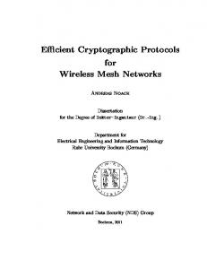
4

b

(c)

b

Figure 1: Example network topology

2

Ad hoc On-Demand Distance Vector Routing Protocol

AODV [79] is a widely-used routing protocol designed for MANETs, and is one of the four protocols currently standardised by the IETF MANET working group9 . It also forms the basis of new WMN routing protocols, including the upcoming IEEE 802.11s wireless mesh network standard [53].

2.1 Basic Protocol AODV is a reactive protocol: routes are established only on demand. A route from a source node s to a destination node d is a sequence of nodes [s, n1 , . . . , nk , d], where n1 , . . . , nk are intermediate nodes located on the path from s to d. Its basic operation can best be explained using a simple example topology shown in Figure 1(a), where edges connect nodes within transmission range. We assume node s wants to send a data packet to node d, but s does not have a valid routing table entry for d. Node s initiates a route discovery mechanism by broadcasting a route request (RREQ) message, which is received by s’s immediate neighbours a and b. We assume that neither a nor b knows a route to the destination node d.10 Therefore, they simply re-broadcast the message, as shown in Figure 1(b). Each RREQ message has a unique identifier which allows nodes to ignore duplicate RREQ messages that they have handled before. When forwarding the RREQ message, each intermediate node updates its routing table and adds a “reverse route” entry to s, indicating via which next hop the node s can be reached, and the distance in number of hops. Once the first RREQ message is received by the destination node d (we assume via a), d also adds a reverse route entry in its routing table, saying that node s can be reached via node a, at a distance of 2 hops. Node d then responds by sending a route reply (RREP) message back to node s, as shown in Figure 1(c). In contrast to the RREQ message, the RREP is unicast, i.e., it is sent to an individual next-hop node only. The RREP is sent from d to a, and then to s, using the reverse routing table entries created during the forwarding of the RREQ message. When processing the RREP message, a node creates a “forward route” entry into its routing table. For example, upon receiving the RREP via a, node s creates an entry saying that d can be reached via a, at a distance of 2 hops. At the completion of the route discovery process, a route has been established from s to d, and data packets can start to flow. In the event of link and route breaks, AODV uses route error (RERR) messages to inform affected nodes. Sequence numbers are another important aspect of AODV, and are used to indicate the freshness of routing table entries for the purpose of preventing routing loops.

2.2 Detailed Examples Each node ip stores and maintains its own sequence number and its own routing table, which consists of exactly one entry for each known destination dip. In this paper we represent a routing table entry as a tuple (dip , dsn , dsk , flag , hops , nhip , pre), indicating that nhip is the next hop on a route to dip of length 9 http://datatracker.ietf.org/wg/manet/charter/ 10 In

case an intermediate node knows a route to d, it directly sends a route reply back.


5

hops; dsn is a sequence number measuring the freshness of this information. The flag dsk indicates if the sequence number is known (kno) or unknown (unk). In the former case the sequence number dsn can be used to measure the freshness; in the latter the value of dsn cannot be used since one cannot “trust” the value. The flag flag indicates if the route is valid (val)—it can be used to forward packets—or if it is outdated (inv). Finally, pre is the set of neighbours who are “interested” in the route to dip—they are expected to use ip as the next hop in their own routes to dip. We illustrate the AODV routing protocol in the example of Figure 2, where AODV is used to establish a route between nodes a and c. The small numbers inside the nodes denote the nodes’ sequence numbers. Initially all these numbers are set to 1. For simplicity, we leave out the last component pre of routing table entries; hence each entry is a 6-tuple here. Figure 2(a) shows the initial state. We assume that node a wants to send a data packet to node c. First, a checks its routing table and finds that it does not have a (valid) routing table entry for the destination node c. In fact its routing table is empty. Therefore it initiates a route discovery process by generating a RREQ message. For ease of explanation, we represent the generated RREQ message as rreq(hops ,rreqid , dip ,dsn ,dsk ,oip ,osn ,sip), indicating that the route request originates from node oip with sequence number osn, searching for a route to destination dip with sequence number at least dsn. This sequence number is taken from the entry for dip in the routing table maintained by node a. If no entry for dip is available, dsn is set to 0. If there is no entry for dip or the sequence number is marked as unknown in the routing table, dsk is set to unk (“unknown”); otherwise it is set to kno (“known”). In addition, hops is the number of hops the message has already travelled from oip, rreqid is the unique identifier of the route request, and sip denotes the sender of the message.11 When generating a new RREQ message, the originator node must increment its own sequence number before copying it into the RREQ message. Therefore, the RREQ message from node a is rreq(0 , rreqid , c , 0 , unk , a , 2 , a). This RREQ message is broadcast to all its neighbours (Figure 2(b)). (a) a wants to send a packet to c.

(b) a broadcasts a new RREQ message; nodes b, d receive the RREQ and update their RTs. (a,2,kno,val,1,a)

b

c

1

1

EQ RR

a

a

1

2

d

b

c

1

1

RR EQ

d 1

1

(a,2,kno,val,1,a)

(c) d forwards the RREQ; node a receives it; b forwards the RREQ; nodes a, c receive it. (a,2,kno,val,1,a)

b EQ RR

(b,0,unk,val,1, b) (d,0,unk,val,1,d)

(a,2,kno,val,1,a) (c ,1,kno,val,1, c)

(a,2,kno,val,2,b) (b ,0,unk,val,1,b)

RREQ

1

(d) c unicasts a RREP message to b.

(a,2,kno,val,2,b) (b ,0,unk,val,1,b)

c

b

1

a 2

RREP

1

(b,0,unk,val,1, b) (d,0,unk,val,1,d)

RR EQ

d

c 1

a 2

d

1

1

(a,2,kno,val,1,a)

(a,2,kno,val,1,a)

Figure 2: Simple example 11 Following the RFC specification of AODV, the sender address sip is not part of the message itself; however a node that receives a message is able to obtain it from the source IP address field in the IP header of the message.


6

(e) b unicasts the RREP to a. (a,2,kno,val,1,a) (c ,1,kno,val,1, c) (a,2,kno,val,2,b) (b ,0,unk,val,1,b)

EP RR

(b,0,unk,val,1, b) (c,1,kno,val,2, b) (d,0,unk,val,1,d)

b

c

1

1

a 2

d 1 (a,2,kno,val,1,a)

Figure 2 (cont’d): Simple example Nodes b and d receive the request and update their routing tables to insert an entry for node a. Since nodes b and d do not know a route to node c (they have no routing table entry with destination c), they both re-broadcast the RREQ message, as shown in Figure 2(c). Before forwarding the message, nodes b and d increment the hops information in the RREQ message from 0 to 1, meaning that the distance to a is now 1. The forwarded RREQ messages from nodes b and d are then received by node a. Through these messages node a knows that nodes b and d are 1-hop neighbours, but node a does not know their sequence numbers, hence they are set to “unknown”. Therefore, node a creates routing table entries for its neighbours, but with unknown sequence number 0, and sequence-number-status flag set to unk. Apart from this, since node a is the originator of the RREQ, it will ignore these messages. The same RREQ message forwarded by node b is also received by node c. Node c reacts by creating routing table entries for both its previous-hop neighbour (node b) and the originator of the RREQ (node a). It then responds by generating a RREP message. Again, for ease of explanation, we represent the RREP message as rrep(hops,dip,dsn,oip,sip), where hops now indicates the distance to dip. As before, sip is the sender of the message. Since the destination node’s sequence number specified in the received RREQ message is unknown (dsn = 0 and dsk = unk), node c copies its own sequence number into the RREP message. Hence the RREP message from node c is rrep(0 , c , 1 , a , c). From node c, the RREP message is unicast back to its previous-hop node b, on the path back towards the originator node a (Figure 2(d)). Node b processes the RREP message and updates its routing table to insert an entry for node c. It also increments the hops information in the RREP message from 0 to 1 before forwarding it to node a (Figure 2(e)). When node a receives the RREP message, this completes the route discovery process and a route is now established from node a to node c. Data packets from node a can now be sent to node c. We next describe a more interesting example of how AODV operates in a changing network topology. In this example, we will show that due to the changing network topology and subsequent updates to the routing table, a route reply message is not necessarily sent back to the node which had forwarded the route request previously. Figure 3(a) shows the initial network topology, and the initial state of the nodes in the topology. We assume that node s wants to send a data packet to node d; hence it generates and broadcasts a route request message RREQ1 (rreq(0 , rreqid , d , 0 , unk , s , 2 , s)), as shown in Figure 3(b). Next, the network topology changes whereby node s is now within transmission range of node d. This change in the network topology can be due to node mobility (i.e., node s moves into transmission range of node d), or due to the improved quality of the wireless link between nodes s and d. Figure 3(d) shows a situation where node s wants to send a data packet to node a, thereby generating and broadcasting a new route request message RREQ2 (rreq(0 , rreqid , a , 0 , unk , s , 3 , s)) destined to node a. Note that


7

RREQ2 is received by node d, which results in the insertion of an entry for node s with sequence number 3 in node d’s routing table. At the same time, the previous route request RREQ1 is forwarded to node b on its path towards node d. (a) The initial state.

(b) s broadcasts a new RREQ message destined to d. b

1

1 RREQ1

b

s

d

a

s

d

a

1

1

1

2

1

1

(c) Network topology changes; s moves into the transmission range of d (d) s broadcasts a new RREQ message destined to a; (e) d forwards RREQ2 ; nodes a, b, s receive it; RREQ1 is forwarded. b updates its routing table entry to s. (d,0,unk,val,1,d) (s,3,kno,val,2,d)

(s,2,kno,val,2,∗)

b

b

1

1

s

RREQ2

RREQ2

RREQ1

RREQ2

3

d

a

s

1

1

3

1

(d,0,unk,val,1,d)

(s,3,kno,val,1,s)

(s,3,kno,val,1,s)

RREQ2

d

RREQ2

a

1 (d,0,unk,val,1,d) (s,3,kno,val,2,d)

(f) All steps that would follow as a reaction to RREQ2 are skipped, because they are not important here. (g) b forwards RREQ1 ; it is received by node d. (h) d generates a reply to RREQ1 ; this reply is not sent back to b; it is sent to s. (d,0,unk,val,1,d) (s,3,kno,val,2,d)

b

b

1

1

RREQ1

RREQ1

(d,0,unk,val,1,d) (s,3,kno,val,2,d)

s

d

a

s

d

a

3

1

3

1

(d,0,unk,val,1,d)

(b,0,unk,val,1,b) (s,3,kno,val,1,s)


(d,1,kno,val,1,d)



RREP1

Figure 3: An example with changing network topology Figure 3(e) shows that node d forwards RREQ2 , which is received by nodes a, b, and s. The subsequent steps in response to RREQ2 , i.e. the generation of a RREP message by node a, and its unicast to node d and subsequent forwarding to the originator node s, are not shown in Figure 3 as they do not contribute towards the objective of this example. Figure 3(g) shows that RREQ1 is forwarded by node b and finally received by the destination node d. Since the destination sequence number for node s in RREQ1 (dsn = 2) is older than the corresponding destination sequence number information in node d’s routing table entry for node s (dsn = 3), the routing table entry for node s is not updated. Node d then generates a RREP message in response to RREQ1 . The destination node d searches in its routing table for a reverse route entry for node s, and finds that the next hop nhip for the route towards node s is node s itself. Therefore, the RREP message is not sent back to node b (from which the RREQ1 message is received), but instead is sent back directly to node s (Figure 3(h)).


3

8

Abstractions Chosen

Our formalisation of AODV tries to accurately model the protocol as defined in the IETF RFC 3561 specification [79]. The model focusses on layer 3 of the protocol stack, i.e., the routing and forwarding of messages and packets, and abstracts from lower layer network protocols and mechanisms such as the Carrier Sense Multiple Access (CSMA) protocol. The presented formalisation includes all core components of the protocol, but, at the moment, abstracts from timing issues and optional protocol features. This keeps our specification manageable. Our plan is to extend our model step by step. Even though our model currently does not cover all aspects, it allows us to point to shortcomings in AODV and to discuss some possible improvements. The model also allows us to reason about protocol behaviour and to prove critical protocol characteristics. In this section, we list all items that are not yet part of our formal model.

3.1 Timing We abstract from all timing issues. Surely, this is a big decision and there are good reasons to add time as a next step. However, this abstraction makes the verification of properties much easier: No entry of a routing table or route reply message has the field lifetime that maintains the expiration or deletion time of the route in AODV. Informally this means that no valid route is set to invalid due to timing, that no invalid route disappears from the routing table (except when it is overwritten), and that we never delete elements of the set rreqs of already seen requests (described in Section 5.6). In terms of the RFC that means that ACTIVE_ROUTE_TIMEOUT, DELETE_PERIOD and PATH_DISCOVERY_TIME are set to infinity.

3.2 Optional Protocol Features A route may be locally repaired if a link break in a valid route occurs. In that case, the node upstream of that break may choose to initiate a local repair if the destination was no farther than MAX_REPAIR_TTL hops away. Local repair is optional; therefore we do not model this feature here. To avoid unnecessary network-wide dissemination of RREQs, the originating node should use an expanding ring search technique. This is again an optional feature, which is not modelled here; we can say that the RING_TRAVERSAL_TIME is set to infinity. A route request may be sent multiple times. This happens if a node, after broadcasting a RREQ, does not receive the corresponding RREP within a given amount of time. In that case the node may broadcast another RREQ, up to a maximum of RREQ_RETRIES. Since the default value for RREQ_RETRIES is only two, and moreover this whole procedure is optional, we have not modelled this resending of RREQ messages. If a route discovery has been attempted RREQ_RETRIES times without receiving any RREP, a destination unreachable message should be delivered to the client (application) hooked up at the originator. This interaction between different layers of the protocol stack has not been modelled here since it is not a core part of the protocol itself. When a node wants to increment its sequence number, but the largest possible number (232 − 1) has already been assigned to it, a sequence number rollover has to be accomplished. This rollover violates the property that sequence numbers are monotonically increased over time; therefore it would be possible to create routing loops. It appears that loops as a consequence of rollover are rare in practice and therefore we decided to model sequence numbers by the unbounded set of natural numbers. Interfaces, as part of routing table entries, store information concerning the network link, e.g., that the node is connected via Ethernet. This is because AODV should operate smoothly over wired as well as

9


wireless networks. Here we assume that nodes have only one type of network interface and consequently leave out this field. Another phenomenon which may yield complications and possibly routing loops, are node crashes. For now, we have neither modelled crashes nor actions after reboot. By default, our process algebra establishes only bidirectional links12 . We will point out how by a trivial change it can model unidirectional links (Section 4). We have decided not to make this our default here, since, by doing so, fundamental properties such as route correctness would not hold for AODV any longer (see Section 7.7). Unidirectional links come along with “blacklist” sets, which we also do not model. We further do not model the optional support for aggregate networks and the use of AODV with other networks, as loosely discussed in Sections 7 and 8 of the AODV RFC [79]. Finally, hello messages can be used as an optional feature to offer connectivity information to a node’s neighbours. Since in our model all optional parts are skipped, we do not model hello messages either; information about 1-hop neighbours is established by receiving AODV control messages.

3.3 Flags Following the RFC [79], AODV control messages and routing table entries have to maintain a series of state and routing flags such as the repair flag, the unknown sequence number flag, and the gratuitous RREP flag. For most of these flags there is no compulsion to ever set them. An exception is the unknown sequence number (‘U’) flag. In some implementations, such as AODV-UU [2], this flag is omitted in favour of a special element denoting the unknown sequence number. In our model, we follow the RFC and model the sequence number as well as the ‘U’ flag. We speak of a sequence-number-status flag, with values “known” and “unknown”. Besides the ‘U’ flag, each route request has the join (‘J’), the repair (‘R’), the gratuitous RREP (‘G’) and the destination only (‘D’) flag. The ‘J’ and ‘R’ flag are reserved for multicast, an optional feature not fully specified in the RFC. We do not model the multicast feature, and hence ignore these two flags. The ‘G’ flag indicates whether a gratuitous RREP should be unicast, by an intermediate node answering the RREQ message, to the destination node of the original message; the ‘D’ flag indicates that only the destination may respond to this RREQ. Both flags may be set when a request is initiated. Since this is also optional, we have decided to skip these features for the moment. However, their inclusion should be straightforward. A route reply carries two flags: the repair (‘R’) flag, used for the multicast feature, and the acknowledgment (‘A’) flag, which indicates that a route reply acknowledgment message must be sent in response to a RREP message. We do not model these flags: the former since we do not model multicast at all; the latter since this flag is optional. Consequently, we have no need to model the route reply acknowledgment (RREP-ACK) message, which—next to RREQ, RREP and RERR—constitutes a fourth kind of AODV control message. Finally, an error message only maintains the no delete (‘N’) flag. It is set if a node has performed a local repair. Since we do not model local repair, we are able to abstract from that flag. Flags pertaining to local repair, but stored in the routing tables, are the repairable and the being repaired flags. For the same reasons, we skip these flags as well.

12 A bidirectional link means that if a node b is in transmission range of a (a can send messages to b), then a is also in range of b. A bidirectional link does not mean that if a knows a route to b, then b knows a route to a.


4

10

A Process Algebra for Wireless Mesh Routing Protocols

In this section we propose AWN (Algebra of Wireless Networks), a process algebra for the specification of WMN routing protocols, such as AODV. It is a variant of standard process algebras [71, 47, 4, 8], adapted to the problem at hand. For example, it allows us to embed data structures. In AWN, a WMN is modelled as an encapsulated parallel composition of network nodes. On each node several sequential processes may be running in parallel. Network nodes communicate with their direct neighbours—those nodes that are in transmission range—using either broadcast or unicast. Our formalism maintains for each node the set of nodes that are currently in transmission range. Due to mobility of nodes and variability of wireless links, nodes can move in or out of transmission range. The encapsulation of the entire network inhibits communications between network nodes and the outside world, with the exception of the receipt and delivery of data packets from or to clients13 of the modelled protocol that may be hooked up to various nodes.

4.1 A Language for Sequential Processes The internal state of a process is determined, in part, by the values of certain data variables that are maintained by that process. To this end, we assume a data structure with several types, variables ranging over these types, operators and predicates. First order predicate logic yields terms (or data expressions) and formulas to denote data values and statements about them.14 Our data structure always contains the types DATA, MSG, IP and P(IP) of application layer data, messages, IP addresses—or any other node identifiers—and sets of IP addresses. We further assume that there is a function newpkt : DATA × IP → MSG that generates a message with new application layer data for a particular destination. The purpose of this function is to inject data to the protocol; details will be given later. In addition, we assume a type SPROC of sequential processes, and a collection of process names, each being an operator of type TYPE1 × · · · × TYPEn → SPROC for certain data types TYPEi . Each process name X comes with a defining equation def

X (var1 , . . . , varn ) = p , in which, for each i = 1, . . . , n, vari is a variable of type TYPEi and p a sequential process expression defined by the grammar below. p may contain the variables vari as well as X ; however, all occurrences of data variables in p have to be bound.15 The choice of the underlying data structure and the process names with their defining equations can be tailored to any particular application of our language; our decisions made for modelling AODV are presented in Sections 5 and 6. The process names are used to denote the processes that feature in this application, with their arguments vari binding the current values of the data variables maintained by these processes. The sequential process expressions are given by the following grammar: SP ::= X (exp1 , . . . , expn ) | [ϕ ]SP | [[var := exp]]SP | SP + SP | α .SP | unicast(dest , ms).SP ◮ SP α ::= broadcast(ms) | groupcast(dests , ms) | send(ms) | deliver(data) | receive(msg) Here X is a process name, expi a data expression of the same type as vari , ϕ a data formula, var := exp an assignment of a data expression exp to a variable var of the same type, dest, dests, data and ms data expressions of types IP, P(IP), DATA and MSG, respectively, and msg a data variable of type MSG. 13 The

application layer that initiates packet sending and awaits receipt of a packet. we also allow partial functions with the convention that any atomic formula containing an undefined subterm evaluates to false. 15 An occurrence of a data variable in p is bound if it is one of the variables var , a variable msg occurring in a subexpression i receive(msg).q, a variable var occurring in a subexpression [[var := exp]]q, or an occurrence in a subexpression [ϕ ]q of a variable occurring free in ϕ . Here q is an arbitrary sequential process expression. 14 As operators


11

broadcast(ξ (ms))

ξ , broadcast(ms).p −−−−−−−−−−→ ξ , p groupcast(ξ (dests),ξ (ms))

ξ , groupcast(dests , ms).p −−−−−−−−−−−−−−→ ξ , p unicast(ξ (dest),ξ (ms))

ξ , unicast(dest , ms).p ◮ q −−−−−−−−−−−−→ ξ , p ¬unicast(ξ (dest),ξ (ms))

ξ , unicast(dest , ms).p ◮ q −−−−−−−−−−−−−→ ξ , q send(ξ (ms))

ξ , send(ms).p −−−−−−−→ ξ , p deliver(ξ (data)) ξ , deliver(data).p − −−−−−−−− → ξ, p

ξ , receive(msg).p −−−−−→ ξ [msg := m], p receive(m)

(∀m ∈ MSG)

τ

ξ , [[var := exp]]p −→ ξ [var := ξ (exp)], p n ′ 0[var / def i := ξ (expi )]i=1 , p −→ ζ , p (X(var1 , . . . , varn ) = p) a ′ ξ , X (exp1 , . . . , expn ) −→ ζ , p a

ξ , p −→ ζ , p′ a ξ , p + q −→ ζ , p′ a

ξ , q −→ ζ , q′ a ξ , p + q −→ ζ , q′ a

(∀a ∈ Act)

ϕ

ξ →ζ τ ξ , [ϕ ]p −→ ζ, p

(∀a ∈ Act)

Table 1: Structural operational semantics for sequential process expressions Given a valuation of the data variables by concrete data values, the sequential process [ϕ ]p acts as p if ϕ evaluates to true, and deadlocks if ϕ evaluates to false. In case ϕ contains free variables that are not yet interpreted as data values, values are assigned to these variables in any way that satisfies ϕ , if possible. The sequential process [[var := exp]]p acts as p, but under an updated valuation of the data variable var. The sequential process p + q may act either as p or as q, depending on which of the two processes is able to act at all. In a context where both are able to act, it is not specified how the choice is made. The sequential process α .p first performs the action α and subsequently acts as p. The action broadcast(ms) broadcasts (the data value bound to the expression) ms to the other network nodes within transmission range, whereas unicast(dest , ms).p ◮ q is a sequential process that tries to unicast the message ms to the destination dest ; if successful it continues to act as p and otherwise as q. In other words, unicast(dest , ms).p is prioritised over q; only if the action unicast(dest , ms) is not possible, the alternative q will happen. It models an abstraction of an acknowledgment-of-receipt mechanism that is typical for unicast communication but absent in broadcast communication, as implemented by the link layer of relevant wireless standards such as IEEE 802.11. The process groupcast(dests , ms).p tries to transmit ms to all destinations dests, and proceeds as p regardless of whether any of the transmissions is successful. Unlike unicast and broadcast, the expression groupcast does not have a unique counterpart in networking. Depending on the protocol and the implementation it can be an iteratively unicast, a broadcast, or a multicast; thus groupcast abstracts from implementation details. The action send(ms) synchronously transmits a message to another process running on the same network node; this action can occur only when this other sequential process is able to receive the message. The sequential process receive(msg).p receives any message m (a data value of type MSG) either from another node, from another sequential process running on the same node or from the client hooked up to the local node. It then proceeds as p, but with the data variable msg bound to the value m. The submission of data from a client is modelled by the receipt of a message newpkt(d,dip), where the function newpkt generates a message containing the data d and the intended destination dip. Data is delivered to the client by deliver(data ). The internal state of a sequential process described by an expression p in this language is determined by p, together with a valuation ξ associating data values ξ (var) to the data variables var maintained


12

by this process. Valuations naturally extend to ξ -closed data expressions—those in which all variables are either bound or in the domain of ξ . The structural operational semantics of Table 1 is in the style of Plotkin [85] and describes how one internal state can evolve into another by performing an action.16 The set Act of actions consists of broadcast(m), groupcast(D , m), unicast(dip , m), ¬unicast(dip , m), send(m), deliver(d), receive(m) and internal actions τ , for each choice of m ∈ MSG, dip ∈ IP, D ∈ P(IP) and d ∈ DATA. Here, ¬unicast(dip , m) denotes a failed unicast. Moreover ξ [var := v] denotes the valuation that assigns the value v to the variable var, and agrees with ξ on all other variables. The empty n valuation 0/ assigns values to no variables. Hence 0[var / i := vi ]i=1 is the valuation that only assigns the values vi to the variables vari for i = 1, . . . , n. The rule for process names in Table 1 (Line 9) says that a process, named X , has the same transitions as the body p of its defining equation. In a p −→ p′ . Adding data variables as arguments of process names would yield CCS [71], such a rule is a X −→ p′ a ′ ξ , p −→ ζ , p . However, a sequential process expression may call a process name with a ξ , X (var1 , . . . , varn ) −→ ζ , p′ data expressions filled in for these variables. This necessitates a translation from a given valuation ξ of the variables that may occur in these data expressions to a new valuation ξ # of the variables vari that occur in the defining equation of X : a ξ # , X (var1 , . . . , varn ) −→ ζ , p′ . a ξ , X (exp1 , . . . , expn ) −→ ζ , p′

Here ξ # (vari ) = ξ (expi ). Moreover, in defining ξ # we drop all bindings of variables other than the vari . Example 4.1 Given the defining equation def

X (numa) = send(numa + 1) . receive(numb) . X (numa + numb) and the valuation given by ξ (numa) = 3 and ξ (numb) = 4, with numa and numb data variables of type IN, we have send(8) ξ , X (numa + numb) −−−−→ ζ , receive(numb) . X (numa + numb) , where ζ (numa) = 7 and ζ (numb) is undefined.

ξ , p[expi /vari ]ni=1 −→ ζ , p′ a ξ , X (exp1 , . . . , expn ) −→ ζ , p′ n where p[expi /vari ]i=1 denotes the expression p in which each variable vari is replaced by the expression expi , for i = 1, . . . , n. This would modify the derivation of Example 4.1 into a

An alternative and more traditional rule for process names would be

ξ , X (numa + numb) −−−−→ ξ , receive(numc) . X (numa + numb + numc) , send(8)

in which one applies α -conversion when renaming the argument numb of receive into numc to avoid a name clash. In this paper we avoid casual application of α -conversion, since in our invariant proofs in Section 7 we track the value of variables that are identified by name only. With this in mind we formulated our rule for process names. The rules defining the choice operator (Table 1, Line 10) are standard and imply immediately that + is associative. ϕ Finally, ξ → ζ says that ζ is an extension of ξ , i.e., a valuation that agrees with ξ on all variables on which ξ is defined, and valuates the other variables occurring free in ϕ , such that the formula ϕ holds under ζ . All variables not free in ϕ and not evaluated by ξ are also not evaluated by ζ . of the transition rules feature statements of the form ξ (exp) where exp is a data expression. Here the application of the rule depends on ξ (exp) being defined. In case ξ (exp) is undefined—either because exp contains a variable that is not in the domain of ξ or because exp contains a partial function that is given an argument for which it is not defined—the transition cannot be taken, possibly leading to a deadlock of the represented process. 16 Eight


13

a

a

P −→ P′ a P hh Q −→ P′ hh Q

Q −→ Q′ a P hh Q −→ P hh Q′

(∀a 6= receive(m)) receive(m)

(∀a 6= send(m))

send(m)

P −−−−−→ P′ Q −−−−→ Q′ τ P hh Q −→ P′ hh Q′

(∀m ∈ MSG)

Table 2: Structural operational semantics for parallel process expressions Example 4.2 Let ξ (numa) = 7 and ξ (numb), ξ (numc) be undefined. Then the sequential process given by the pair ξ , [numa = numb + numc]p admits several transitions of the form τ

ξ , [numa = numb + numc]p −→ ζ , p such as the one with ζ (numb) = 2 and ζ (numc) = 5. On the other hand, ξ , [numa = numb + 8]p admits no transitions, since numb ∈ IN.

4.2 A Language for Parallel Processes Parallel process expressions are given by the grammar PP ::= ξ , SP | PP hh PP where SP is a sequential process expression and ξ a valuation. An expression ξ , p denotes a sequential process expression equipped with a valuation of the variables it maintains. The process P hh Q is a parallel composition of P and Q, running on the same network node. As formalised in Table 2, an action receive(m) of P synchronises with an action send(m) of Q into an internal action τ . These receive actions of P and send actions of Q cannot happen separately. All other actions of P and Q, including receive actions of Q and send actions of P, occur interleaved in P hh Q. Thus, in an expression (P hh Q) hhR, for example, the send and receive actions of Q can communicate only with P and R, respectively, but the receive actions of R, as well as the send actions of P, remain available for communication with the environment. Therefore, a parallel process expression denotes a parallel composition of sequential processes ξ , P with information flowing from right to left. The variables of different sequential processes running on the same node are maintained separately, and thus cannot be shared. Instead of introducing the novel operator hh, we could have used the partially synchronous parallel composition operator k of ACP [4], | of CCS [71] or kA of CSP [77]. However, those operators are normally used in conjunction with restriction and/or concealment operators, which are not needed when using hh. In ACP a restriction or encapsulation operator is used to prevent read and send actions of the components of a parallel composition to occur by themselves, without synchronising with an action from another other component. Furthermore, a concealment or abstraction operator is used to convert the results of successful synchronisation into internal actions, thereby making sure that they will not take part in further synchronisations with the environment. In CCS, the concealment operator is not needed, as the parallel composition directly produces internal actions as the results of synchronisation; however, the restriction operator is indispensable. In CSP, on the other hand, the restriction operator is made redundant by incorporating its function within the parallel composition. In this framework matching read and send actions have the same name, which is also the name of the result of their synchronisation. This makes the concealment operator indispensable. It appears to be impossible to combine the ideas of CCS and CSP directly to make both the restriction and the concealment operator redundant, while maintaining associativity of the parallel composition. Our operator hh is the first that does not need such auxiliary operators, sacrificing commutativity, but not associativity, to make this possible.


14

Though hh only allows information flow in one direction, it reflects reality of WMNs. Usually two sequential processes run on the same node: P hh Q. The main process P deals with all protocol details of the node, e.g., message handling and maintaining the data such as routing tables. The process Q manages the queueing of messages as they arrive; it is always able to receive a message even if P is busy. The use of message queueing in combination with hh is crucial, since otherwise incoming messages would be lost when the process is busy dealing with other messages17 , which would not be an accurate model of what happens in real implementations.

4.3 A Language for Networks We model network nodes in the context of a wireless mesh network by node expressions of the form ip : PP : R. Here ip ∈ IP is the address of the node, PP is a parallel process expression, and R ∈ P(IP) is the range of the node—the set of nodes that are currently within transmission range of ip. groupcast(D,m)

P −−−−−−−→ P′

broadcast(m)

P −−−−−−−−→ P′

R : *cast(m)

ip : P : R −−−−−−−−→ ip : P′ : R

R∩D : *cast(m)

ip : P : R −−−−−−→ ip : P′ : R unicast(dip,m)

P −−−−−−−−→ P′

¬unicast(dip,m)

P −−−−−−−−→ P′

dip ∈ R

dip 6∈ R

τ

ip : P : R −−−−−−−−→ ip : P′ : R

{dip} : *cast(m)

ip : P : R −→ ip : P′ : R

P −−−−−→ P′

deliver(d)

P −−−−−→ P′

ip : deliver(d)

ip : P : R −−−−−−−−−−→ ip : P′ : R

receive(m)

{ip}¬0/ : arrive(m)

ip : P : R −−−−−−−→ ip : P′ : R τ

P −→ P′ τ ip : P : R −→ ip : P′ : R

0¬{ip} / : arrive(m)

ip : P : R −−−−−−−−−− → ip : P : R

connect(ip,ip′ )

ip : P : R −−−−−−−−−→ ip : P : R − {ip′ }

ip : P : R −−−−−−−−→ ip : P : R ∪ {ip′ }

connect(ip′ ,ip)

ip : P : R −−−−−−−−−→ ip : P : R − {ip′ }

ip 6∈ {ip′, ip′′ }

ip 6∈ {ip′, ip′′ }

ip : P : R −−−−−−−−→ ip : P : R ∪ {ip′ }

connect(ip′,ip′′ )

ip : P : R −−−−−−−−→ ip : P : R

disconnect(ip,ip′ )

disconnect(ip′ ,ip)

disconnect(ip′,ip′′ )

ip : P : R −−−−−−−−−−→ ip : P : R

Table 3: Structural operational semantics for node expressions A partial network is then modelled by a parallel composition k of node expressions, one for every node in the network, and a complete network is a partial network within an encapsulation operator [ ] that limits the communication of network nodes and the outside world to the receipt and the delivery of data packets to and from the application layer attached to the modelled protocol in the network nodes. This yields the following grammar for network expressions: N ::= [M]

M ::= ip : PP : R | MkM .

The operational semantics of node and network expressions of Tables 3 and 4 uses transition labels R : *cast(m), H¬K : arrive(m), connect(ip, ip′ ), disconnect(ip, ip′ ), ip : newpkt(d, dip), ip : deliver(d) and τ . As before, m ∈ MSG, d ∈ DATA, R ∈ P(IP), and ip, ip′ ∈ IP. Moreover, H, K ∈ P(IP) are 17 assuming

that one employs the optional augmentation of Section 4.5


15 R : *cast(m)

H¬K : arrive(m) N −−−−−−−−−→ N ′ H ⊆ R

M −−−−−−→ M ′

H¬K : arrive(m)

M −−−−−−−−− → M′

K ∩ R = 0/

R :*cast(m)

MkN −−−−−−→ M ′ kN ′

H¬K : arrive(m)

M −−−−−−−−− → M′

R : *cast(m) N −−−−−−→ N ′ H ⊆ R

K ∩ R = 0/

R : *cast(m)

MkN −−−−−−→ M ′ kN ′ H ′ ¬K ′ : arrive(m)

N −−−−−−−−−→ N ′

(H∪H ′ )¬(K∪K ′ ) : arrive(m)

MkN −−−−−−−−−−−−−−−→ M ′ kN ′ M −−−−−−−→ M ′

ip : deliver(d)

N −−−−−−−→ N ′

ip : deliver(d)

MkN −−−−−−−→ MkN ′

ip : deliver(d)

MkN −−−−−−−→ M ′ kN connect(ip,ip′ )

M −−−−−−−−→ M ′

ip : deliver(d)

connect(ip,ip′ )

N −−−−−−−−→ N ′

connect(ip,ip′ )

MkN −−−−−−−−→ M ′ kN ′ disconnect(ip,ip′ )

M −−−−−−−−→ M ′

connect(ip,ip′ )

M −−−−−−−−−→ M ′

connect(ip,ip′ )

[M] −−−−−−−−−→ [M ′ ]

[M] −−−−−−−−→ [M ′ ]


τ

M −→ M ′ τ MkN −→ M ′ kN disconnect(ip,ip′ )

M −−−−−−−−−→ M ′

τ

N −→ N ′ τ MkN −→ MkN ′ disconnect(ip,ip′ )

N −−−−−−−−−→ N ′


MkN −−−−−−−−−→ M ′ kN ′ R : *cast(m)

M −−−−−−→ M ′ τ [M] −→ [M ′ ]

τ

M −→ M ′ τ [M] −→ [M ′ ]

{ip}¬K : arrive(newpkt(d,dip))

M −−−−−−−→ M ′

ip : deliver(d)

M −−−−−−−−−−−−−−−−−→ M ′

ip : deliver(d)

[M] −−−−−−−−−→ [M ′ ]

[M] −−−−−−−→ [M ′ ]

ip : newpkt(d,dip)

Table 4: Structural operational semantics for network expressions sets of IP addresses. The action R : *cast(m) casts a message m that can be received by the set R of network nodes. We do not distinguish whether this message has been broadcast, groupcast or unicast—the differences show up merely in the value of R. Recall that D ∈ P(IP) denotes a set of intended destinations, and dip ∈ IP a single destination. A failed unicast attempt on the part of its process is modelled as an internal action τ on the part of a node expression. The action send(m) of a process does not give rise to any action of the corresponding node—this action of a sequential process cannot occur without communicating with a receive action of another sequential process running on the same node. The action H¬K : arrive(m) states that the message m simultaneously arrives at all addresses ip ∈ H, and fails to arrive at all addresses ip ∈ K. The rules of Table 4 let a R : *cast(m)-action of one node synchronise with an arrive(m) of all other nodes, where this arrive(m) amalgamates the arrival of message m at the nodes in the transmission range R of the *cast(m), and the non-arrival at the other nodes. The rules for arrive(m) in Table 3 state that arrival of a message at a node happens if and only if the node receives it, whereas non-arrival can happen at any time. This embodies our assumption that, at any time, any message that is transmitted to a node within range of the sender is actually received by that node. (The eighth rule in Table 3, having no premises, may appear to say that any node ip has the option to disregard any message at any time. However, the encapsulation operator (below) prunes away all such disregard-transitions that do not synchronise with a cast action for which ip is out of range.) Internal actions τ and the action ip : deliver(d) are simply inherited by node expressions from the processes that run on these nodes, and are interleaved in the parallel composition of nodes that makes up a network. Finally, we allow actions connect(ip, ip′ ) and disconnect(ip, ip′ ) for ip, ip′ ∈ IP modelling a change in network topology. Each node needs to synchronise with such an action. These actions can be thought of as occurring nondeterministically, or as actions instigated by the environment of the modelled network protocol. In this formalisation node ip′ is in the range of node ip, meaning that ip′ can receive messages sent by ip, if and only if ip is in the range of ip′ . To break this symmetry, one just skips the last four rules of Table 3 and replaces the synchronisation rules for connect and disconnect in Table 4 by interleaving rules (like the ones for deliver and τ ).


16

The main purpose of the encapsulation operator is to ensure that no messages will be received that have never been sent. In a parallel composition of network nodes, any action receive(m) of one of the nodes ip manifests itself as an action H¬K : arrive(m) of the parallel composition, with ip ∈ H. Such actions can happen (even) if within the parallel composition they do not communicate with an action *cast(m) of another component, because they might communicate with a *cast(m) of a node that is yet to be added to the parallel composition. However, once all nodes of the network are accounted for, we need to inhibit unmatched arrive actions, as otherwise our formalism would allow any node at any time to receive any message. One exception however are those arrive actions that stem from an action receive(newpkt(d , dip)) of a sequential process running on a node, as those actions represent communication with the environment. Here, we use the function newpkt, which we assumed to exist.18 It models the injection of new data d for destination dip. The encapsulation operator passes through internal actions, as well as delivery of data to destination nodes, this being an interaction with the outside world. *cast(m)-actions are declared internal actions at this level; they cannot be steered by the outside world. The connect and disconnect actions are passed through in Table 4, thereby placing them under control of the environment; to make them nondeterministic, their rules should have a τ -label in the conclusion, or alternatively connect(ip, ip′ ) and disconnect(ip, ip′ ) should be thought of as internal actions. Finally, actions arrive(m) are simply blocked by the encapsulation—they cannot occur without synchronising with a *cast(m)—except for {ip}¬K : arrive(newpkt(d , dip)) with d ∈ DATA and dip ∈ IP. This action represents new data d that is submitted by a client of the modelled protocol to node ip, for delivery at destination dip.

4.4 Results on the Process Algebra Our process algebra admits translation into one without data structures (although we cannot describe the target algebra without using data structures). The idea is to replace any variable by all possible values it can take. Formally, processes ξ , p are replaced by Tξ (p), where Tξ is defined inductively by Tξ (broadcast(ms) . p) = broadcast(ξ (ms)) . Tξ (p) , Tξ (groupcast(dests , ms) . p) = groupcast(ξ (dests) , ξ (ms)) . Tξ (p) , Tξ (unicast(dest , ms) . p ◮ q) = unicast(ξ (dest) , ξ (ms)) . Tξ (p) ◮ Tξ (q) , Tξ (send(ms) . p) = send(ξ (ms)) . Tξ (p) , Tξ (deliver(data) . p) = deliver(ξ (data)) . Tξ (p) , Tξ (receive(msg) . p) = ∑m∈MSG receive(m) . Tξ [msg:=m] (p) , Tξ ([[var := exp]]p) = τ . Tξ [var:=ξ (exp)] (p) , Tξ ([ϕ ]p) = ∑{ζ |ξ → ϕ τ . Tζ (p) , ζ} Tξ (p + q) = Tξ (p) + Tξ (q) , Tξ (X (exp1 , . . . , expn )) = Xξ (exp1 ),...,ξ (expn ) . The last equation requires the introduction of a process name X~v for every substitution instance ~v of the arguments of X . The resulting process algebra has a structural operational semantics in the de Simone format, generating the same transition system—up to strong bisimilarity, ↔ —as the original. Only the rules for sequential process expressions are different; these are displayed in Table 5. It follows that ↔, and many other semantic equivalences, are congruences on our language. Theorem 4.3 Strong bisimilarity is a congruence for all operators of our language. This is a deep result that usually takes many pages to establish (e.g., [94]). Here we get it directly from the existing theory on structural operational semantics, as a result of carefully designing our language within the disciplined framework described by de Simone [20]. ⊔ ⊓ 18

To avoid the function newpkt we could have introduced a new primitive newpkt, which is dual to deliver.


17 broadcast(m)

send(m)

broadcast(m).p −−−−−−−→ p

send(m).p −−−−→ p

groupcast(D,m)

deliver(d).p −−−−−→ p

unicast(dip,m)

receive(m).p −−−−−→ p

groupcast(D , m).p −−−−−−−−→ p

deliver(d)

receive(m)

unicast(dip , m).p ◮ q −−−−−−−−→ p ¬unicast(dip,m)

a

τ

unicast(dip , m).p ◮ q −−−−−−−−→ q

τ .p −→ p

a

pi −→ p′ a ∑i∈I pi −→ p′

p −→ p′ def (X = p) a ′ X −→ p

a

p −→ p′ a p + q −→ p′

q −→ q′ a p + q −→ q′

a

(∀a ∈ Act)

Table 5: Structural operational semantics for sequential processes after elimination of data structures Theorem 4.4 hh is associative, and k is associative and commutative, up to ↔. Proof. The operational rules for these operators fit a format presented in [17], guaranteeing associativity up to ↔. The ASSOC-de Simone format of [17] applies to all transition system specifications (TSSs) in de Simone format, and allows 7 different types of rules (named 1–7) for the operators in question. Our TSS is in De Simone format; the three rules for hh of Table 2 are of types 1, 2 and 7, respectively. To be precise, it has rules 1a for a ∈ Act − {receive(m) | m ∈ MSG}, rules 2a for a ∈ Act − {send(m) | m ∈ MSG}, and rules 7(a,b) for (a, b) ∈ {(receive(m), send(m)) | m ∈ MSG}. Moreover, the partial communication function γ : Act × Act ⇀ Act is given by γ (receive(m), send(m)) = τ . The main result of [17] is that an operator is guaranteed to be associative, provided that γ is associative and six conditions are fulfilled. In the absence of rules of types 3, 4, 5 and 6, five of these conditions are trivially fulfilled, and the remaining one reduces to 7(a,b) ⇒ (1a ⇔ 2b ) ∧ (2a ⇔ 2γ (a,b) ) ∧ (1b ⇔ 1γ (a,b) ) . Here 1a says that rule 1a is present, etc. This condition is met for hh because the antecedent holds only when taking (a, b) = (receive(m), send(m)) for some m ∈ MSG. In that case 1a is false, 2b is false, and 2a , 2τ , 1b and 1τ are true. Moreover, γ (γ (a, b), c) and γ (a, γ (b, c)) are never defined, thus making γ trivially associative. The argument for k being associative proceeds likewise. Here the only non-trivial condition is the associativity of γ , given by

γ (R : *cast(m), H¬K : arrive(m)) = γ (H¬K : arrive(m), R : *cast(m)) = R : *cast(m) , provided H ⊆ R and K ∩ R = 0, / and

γ (H¬K : arrive(m), H ′¬K ′ : arrive(m)) = (H ∪ H ′)¬(K ∪ K ′) : arrive(m) . Commutativity of k follows by symmetry.

⊔ ⊓

4.5 Optional Augmentation to Ensure Non-Blocking Broadcast Our process algebra, as presented above, is intended for networks in which each node is input enabled [61], meaning that it is always ready to receive any message, i.e., able to engage in the transition receive(m) for any m ∈ MSG. In our model of AODV (Section 6) we will ensure this by equipping each node with a message queue that is always able to accept messages for later handling—even when the main sequential process is currently busy. This makes our model non-blocking, meaning that no sender can be delayed in transmitting a message simply because one of the potential recipients is not ready to receive it. However, the operational semantics does allow blocking if one would (mis)use the process algebra to model nodes that are not input enabled. This is a logical consequence of insisting that any broadcast message is received by all nodes within transmission range.


18

Since the possibility of blocking can regarded as a bad property of broadcast formalisms, one may wish to take away the expressiveness of the language that allows modelling a blocking broadcast. This is the purpose of the following optional augmentations of our operational semantics. The first possibility is the addition of the rule receive(m)

P −−−−−−6→

.

{ip}¬0/ : arrive(m)

ip : P : R −−−−−−−−−− → ip : P : R It states that a message may arrive at a node ip regardless whether the node is ready to receive it; if it is not ready, the message is simply ignored, and the process running on the node remains in the same state. A variation on the same idea stems from the Calculus of Broadcasting Systems (CBS) [88]. It consists in eliminating the negative premise in the above rule in favour of actions ignore(m) ∈ Act—in [88] called discard actions w: —which can be performed by a process exactly when it is not ready to do a receive(m). The rule above then becomes ignore(m) P −−−−−→ P′ {ip}¬0/ : arrive(m)

ip : P : R −−−−−−−−−−→ ip : P′ : R and we need the extra rules:

ξ , broadcast(ms).p −−−−−→ ξ , broadcast(ms).p ignore(m)

ignore(m) ξ , groupcast(dests , ms).p − −−−−→ ξ , groupcast(dests , ms).p

ξ , unicast(dest , ms).p ◮ q −−−−−→ ξ , unicast(dest , ms).p ◮ q ignore(m)

ξ , send(ms).p −−−−−→ ξ , send(ms).p ignore(m)

ignore(m) ξ , deliver(data).p − −−−−→ ξ , deliver(data).p

ξ , [[var := exp]]p −−−−−→ ξ , [[var := exp]]p ignore(m)

ξ , [ϕ ]p −−−−−→ ξ , [ϕ ]p ignore(m)

ξ , p −−−−−→ ξ , p′ ignore(m)

ξ , q −−−−−→ ξ , q′ ignore(m)

ξ , p + q −−−−−→ ξ , p′ + q′ for all m ∈ MSG. Furthermore, the first rule for hh from Table 3 is replaced by ignore(m)

a

P −→ P′ a P hh Q −→ P′ hh Q

(∀a 6= receive(m), ignore(m)). ignore(m)

receive(m)

These rules ensure that for all P and m we always have P −−−−−→ Q ⇔ (Q = P ∧ P −−−−−−6→). After elimination of the data structures as described in Section 4.5, this operational semantics is again in the de Simone format. Either of these two optional augmentations of our semantics gives rise to the same transition system. Moreover, when modelling networks in which all nodes are input enabled—as we do in this paper— the added rule for node expressions will never be used, and the resulting transition system is the same whether we use augmentation or not.

4.6 Illustrative Example To illustrate the use of our process algebra AWN, we consider a network of two nodes a and b (a, b ∈ IP) on which the same process is running, although starting in different states. The process describes a


19

simply (toy-)protocol: whenever a new data packet for destination dip “appears”,19 the data is broadcast through the network until it finally reaches dip. A node alternates between broadcasting, and receiving and handling a message. The data stemming from a message received by node ip will be delivered to the application layer if the message is destined for ip itself. Otherwise the node forwards the message. Every message travelling through the network and handled by the protocol has the form mg(data, dip), where data ∈ DATA is the data to be sent and dip ∈ IP is its destination. The behaviour of each node can be modelled by: def

X(ip , data , dip) = broadcast(mg(data, dip)).Y(ip) def

Y(ip) = receive(m).([m=mg(data, dip) ∧ dip=ip]deliver(data).Y(ip) +[m=mg(data, dip) ∧ dip6=ip]X(ip , data , dip)) . If a node is in a state X(ip , data , dip), where ip ∈ IP is the node’s stored value of its ow IP address, it will broadcast mg(data, dip) and continue in state Y(ip), meaning that all information about the message is dropped. If a node in state Y(ip) receives a message m—a value that will be assigned to the variable m—it has two ways to continue: process [m=mg(data, dip) ∧ dip=ip] deliver(data).Y(ip) is enabled if the incoming message has the form mg(data, dip) and the node itself is the destination of the message (dip=ip). In that case the data distilled from m will be delivered to the application layer, and the process returns to Y(ip). Alternatively, if [m=mg(data, dip)∧dip6=ip], the process continues as X(ip , data,dip), which will then broadcast another message with contents data and dip. Note that calls to processes use expressions as parameters. Let us have a look at three scenarios. First, assume that the nodes a and b are within transmission range of each other; node a in state X(a , d , a), and node b in Y(b). This is formally expressed as [a : X(a , d ,a) :{b}k b : Y(b) :{a}], although for compactness of presentation, we just write [X(a , d ,a) k Y(b)] below. In this case, node a broadcasts the message mg(d, a) and continues as Y(a). Node b receives the message, and continues (after evaluation of the message) as X(b , d , a). Next b broadcasts (forwards) the message, and continues as Y(b), while node a receives mg(d, b), and, due to evaluation, delivers d and continues as Y(a). Formally, we get transitions from one state to the other: a:*cast(mg(d,a))

τ

b:*cast(mg(d,a))

τ

a:deliver(d)

[X(a , d , a) k Y(b)] −−−−−−−−−→−→ [Y(a) k X(b , d , a)] −−−−−−−−−→−→−−−−−−→ [Y(a) k Y(b)]. Here, the τ -transitions are the actions of evaluating one of the two guards of a process Y, and we left out three intermediate expressions. Second, assume that the nodes are not within transmission range, with the initial process of a and b the same as above; formally [a : X(a , d , a) : 0/ k b : Y(b) : 0]. / As before, node a broadcasts mg(d, a) and continues in Y(a); but this time the message is not received by any node; hence no message is forwarded or delivered and both nodes end up running process Y. For the last scenario, we assume that a and b are within transmission range and that they have the initial states X(a , d , b) and X(b , e , a). Without the augmentation of Section 4.5, the network expression [X(a , d , b) k X(b , e , a)] admits no transitions at all; neither node can broadcast its message, because the other node is not listening. With the optional augmentation, assuming that node a sends first: a:*cast((mg(d,b))

b:*cast(mg(e,a))

τ

a:deliver(e)

[X(a , d , b) k X(b , e , a)] −−−−−−−−−→ [Y(a) k X(b , e , a)] − −−−−−−−−→−→−−−−−−→ [Y(a) k Y(b)]. Unfortunately, node b is initially in a state where it cannot receive a message, so a’s message “remains unheard” and b will never deliver that message. To avoid this behaviour, and ensure that both messages get delivered, as happens in real WMNs, a message queue can be introduced (see Section 6.6). Using a message queue, the optional augmentation is not needed, since any node is always in a state where it can receive a message. 19 In this small example, we assume that new data packets just appear “magically”; of course one could use the message newpkt(data ,dip) instead.


5

20

Data Structure for AODV

In this section we set out the basic data structure needed for the detailed formal specification of AODV. As well as describing types for the information handled at the nodes during the execution of the protocol we also define functions which will be used to describe the precise intention—and overall effect—of the various update mechanisms in an AODV implementation. The definitions are grouped roughly according to the various “aspects” of AODV and the host network.

5.1 Mandatory Types As stated in the previous section, the data structure always consists of application layer data, messages, IP addresses and sets of IP addresses. (a) The ultimate purpose of AODV is to deliver application layer data. The type DATA describes a set of application layer data items. An item of data is thus a particular element of that set, denoted by the variable data ∈ DATA. (b) Messages are used to send information via the network. In our specification we use the variable msg of the type MSG. We distinguish AODV control messages (route request, route reply, and route error) as well as data packets: messages for sending application layer data (see Section 5.8). (c) The type IP describes a set of IP addresses or, more generally, a set of node identifiers. In the RFC 3561 [79], IP is defined as the set of all IP addresses. We assume that each node has a unique identifier ip ∈ IP. Moreover, in our model, each node ip maintains a variable ip which always has the value ip. In any AODV control message, the variable sip holds the IP address of the sender, and if the message is part of the route discovery process—a route request or route reply message—we use oip and dip for the origin and destination of the route sought. Furthermore, rip denotes an unreachable destination and nhip the next hop on some route.

5.2 Sequence Numbers As explained in Section 2, any node maintains its own sequence number— the value of the variable sn— and a routing table whose entries describe routes to other nodes. The value of sn increases over time. AODV equips each routing table entry with a sequence number to constitute a measure approximating the relative freshness of the information held—a smaller number denotes older information. All sequence numbers of routes to dip ∈ IP stored in routing tables are ultimately derived from dip’s own sequence number at the time such a route was discovered. We denote the set of sequence numbers by SQN and assume it to be totally ordered. By default we take SQN to be IN, and use standard functions such as max. The initial sequence number of any node is 1. We reserve a special element 0 ∈ SQN to be used for the sequence number of a route, whose semantics is that no sequence number for that route is known. Sequence numbers are incremented by the function inc : SQN → SQN sn + 1 if sn 6= 0 inc(sn) = sn otherwise . The variables osn, dsn and rsn of type SQN are used to denote the sequence numbers of routes leading to the nodes oip, dip and rip. AODV tags sequence numbers of routes as “known” or “unknown”. This indicates whether the value of the sequence number can be trusted. The sequence-number-status flag is set to unknown (unk) when a routing table entry is updated with information that is not equipped with a sequence number itself. In


21

such a case the old sequence number of the entry is maintained; hence the value unk does not indicate that no sequence number for the entry is known. Here we use the set K = {kno, unk} for the possible values of the sequence-number-status flag; we use the variable dsk to range over type K.

5.3 Modelling Routes In a network, pairs (ip0 , ipk ) ∈ IP × IP of nodes are considered to be “connected” if ip0 can send to ipk directly, i.e., ip0 is in transmission range of ipk and vice versa. We say that such nodes are connected by a single hop. When ip0 is not connected to ipk then messages from ip0 directed to ipk need to be “routed” through intermediate nodes. We say that a route (from ip0 to ipk ) is made up of a sequence [ip0 , ip1 , ip2 , . . . , ipk−1 , ipk ], where (ipi , ipi+1 ), i = 0, . . . , k−1, are connected pairs; the length or hop count of the route is the number of single hops, and any node ipi needs only to know the “next hop” address ipi+1 in order to be able to route messages intended for the final destination ipk . In operation, routes to a particular destination are requested and, when finally established, need to be re-evaluated in regard to their “validity”. Routes may become invalid if one of the pairs (ipi , ipi+1 ) in the hop-to-hop sequence gets disconnected. Then AODV may be reinvoked, as the need arises, to discover alternative routes. Meanwhile, an invalid route remains invalid until fresh information is received which establishes a valid replacement route. In addition to the next hop and hop count, AODV also “tags” a route with its validity, sequence number and sequence-number status. For every route, a node moreover stores a list of precursors, modelled as a set of IP addresses. This set collects all nodes which are currently potential users of the route, and are located one hop further “upstream”. When the interest of other nodes emerges, these nodes are added to the precursor list20 ; the main purpose of recording this information is to inform those nodes when the route becomes invalid. In summary, following the RFC, a routing table entry (or entry for short) is given by 7 components: (a) The destination IP address, which is an element of IP; (b) The destination sequence number—an element of SQN; (c) The sequence-number-status flag—an element of the set K = {kno, unk}; (d) A flag tagging the route as being valid or invalid—an element of the set F = {val, inv}. We use the variable flag to range over type F; (e) The hop count, which is an element of IN. The variable hops ranges over the type IN and we make use of the standard function +1; (f) The next hop, which is again an element of IP; and (g) A precursor list, which is modelled as an element of P(IP).21 We use the variable pre to range over P(IP). We denote the type of routing table entries by R, use the variable r, and define a generation function ( , , , , , , ) : IP × SQN × K × F × IN×IP × P(IP) → R . A tuple (dip , dsn , dsk , flag , hops , nhip , pre) describes a route to dip of length hops and validity flag; the very next node on this route is nhip; the last time the entry was updated the destination sequence number was dsn; dsk denotes whether the sequence number is “outdated” or can be used to reason about freshness of the route. Finally, pre is a set of all neighbours who are “interested” in the route to dip. A 20 The 21 The

RFC does not mention a situation where nodes are dropped from the list, which seems curious. word “precursor list” is used in the RFC, but no properties of lists are used.


22

node being “interested” in the route is somewhat sketchily defined as one which has previously used the current node to route messages to dip. Interested nodes are recorded in case the route to dip should ever become invalid, so that they may subsequently be informed. We use projections π1 , . . . π7 to select the corresponding component from the 7-tuple: For example, π6 : R → IP determines the next hop.

5.4 Routing Tables Nodes store all their information about routes in their routing tables; a node ip’s routing table consists of a set of routing table entries, exactly one for each known destination. Thus, a routing table is defined as a set of entries, with the restriction that each has a different destination dip, i.e., the first component of each entry in a routing table is unique.22 Formally, we define the type RT of routing tables by RT := {rt | rt ∈ P(R) ∧ ∀r, s ∈ rt : r 6= s ⇒ π1 (r) 6= π1 (s)} . In the specification and implementation of AODV during route finding nodes choose between alternative routes if necessary to ensure that only one route per destination ends up in their routing table. In our model, each node ip maintains a variable rt, whose value is the current routing table of the node. In the formal model (and indeed in any AODV implementation) we need to extract the components of the entry for any given destination from a routing table. To this end, we define the following partial functions—they are partial because the routing table need not have an entry for the given destination. We begin by selecting the entry in a routing table corresponding to a given destination dip:

σroute : RT × IP ⇀ R r if r ∈ rt ∧ π1 (r) = dip σroute (rt , dip) := undefined otherwise . Through the projections π1 , . . . , π7 , defined above, we can now select the components of a selected entry: (a) The destination sequence number relative to the destination dip: sqn : RT × IP → SQN π2 (σroute (rt , dip)) if σroute (rt , dip) is defined sqn(rt , dip) := 0 otherwise (b) The “known” status of the sequence number of a route: sqnf : RT × IP → K π3 (σroute (rt , dip)) if σroute (rt , dip) is defined sqnf(rt , dip) := unk otherwise (c) The validity status of a recorded route: flag : RT × IP ⇀ F flag(rt , dip) := π4 (σroute (rt , dip)) (d) The hop count of the route from the current node (hosting rt) to dip: dhops : RT × IP ⇀ IN dhops(rt , dip) := π5 (σroute (rt , dip)) 22 As an alternative to restricting the set, we could have defined routing tables as partial functions from IP to R, in which case it makes more sense to define an entry as a 6-tuple, not including the the destination IP as the first component.


23

(e) The identity of the next node on the route to dip (if such a route is known): nhop : RT × IP ⇀ IP nhop(rt , dip) := π6 (σroute (rt , dip)) (f) The set of precursors or neighbours interested in using the route from ip to dip: precs : RT × IP ⇀ P(IP) precs(rt , dip) := π7 (σroute (rt , dip)) The domain of these partial functions changes during the operation of AODV as more routes are discovered and recorded in the routing table rt. The first two functions are extended to be total functions: whenever there is no route to dip inside the routing table under consideration, the sequence number is set to “unknown” (0) and the sequence-number-status flag is set to “unknown” (unk), respectively. In the same style each partial function could be turned into a total one. However, in the specification we use these functions only when they are defined. We are not only interested in information about a single route, but also in general information on a routing table: (a) The set of destination IP addresses for valid routes in rt is given by vD : RT → P(IP) vD(rt) := {dip | (dip , ∗ , ∗ , val , ∗ , ∗ , ∗) ∈ rt} (b) The set of destination IP addresses for invalid routes in rt is iD : RT → P(IP) iD(rt) := {dip | (dip , ∗ , ∗ , inv , ∗ , ∗ , ∗) ∈ rt} (c) Last, we define the set of destination IP addresses for known routes by kD : RT → P(IP) kD(rt) := vD(rt) ∪ iD(rt) = {dip | (dip , ∗ , ∗ , ∗ , ∗ , ∗ , ∗) ∈ rt} Obviously, the partial functions σroute , flag, dhops, nhop and precs are defined for rt and dip exactly when dip ∈ kD(rt).

5.5 Updating Routing Tables Routing tables can be updated for three principal reasons. The first is when a node needs to adjust its list of precursors relative to a given destination; the second is when a received request or response carries information about network connectivity; and the last when information is received to the effect that a previously valid route should now be considered invalid. We define an update function for each case. 5.5.1

Updating Precursor Lists

Recall that the precursors of a given node ip relative to a particular destination dip are the nodes that are “interested” in a route to dip via ip. The function addpre takes a routing table entry and a set of IP addresses npre and updates the entry by adding npre to the list of precursors already present: addpre : R × P(IP) → R addpre((dip , dsn , dsk , flag , hops , nhip , pre) , npre) := (dip , dsn , dsk , flag , hops , nhip , pre ∪ npre) .


24

Often it is necessary to add precursors to an entry of a given routing table. For that, we define the function addpreRT, which takes a routing table rt, a destination dip and a set of IP addresses npre and updates the entry with destination dip by adding npre to the list of precursors already present. It is only defined if an entry for destination dip exists. addpreRT : RT × IP × P(IP) ⇀ RT addpreRT(rt , dip , npre) := (rt − {σroute (rt , dip)}) ∪ {addpre(σroute (rt , dip) , npre)} . Formally, we remove the entry with destination dip from the routing table and insert a new entry for that destination. This new entry is the same as before—only the precursors have been added. 5.5.2

Inserting New Information in Routing Tables

If a node gathers new information about a route to a destination dip, then it updates its routing table depending on its existing information on a route to dip. If no route to dip was known at all, it inserts a new entry in its routing table recording the information received. If it already has some (partial) information then it may update this information, depending on whether the new route is fresher or shorter than the one it has already. We define an update function update(rt , r) of a routing table rt with an entry r only when r is valid, i.e., π4 (r) = val, π2 (r) = 0 ⇔ π3 (r) = unk, and π3 (r) = unk ⇒ π5 (r) = 1.23 update : RT × R ⇀ RT  rt ∪ {r} if π1 (r) 6∈ kD(rt)      nrt ∪ {nr} if π1 (r) ∈ kD(rt) ∧ sqn(rt , π1 (r)) < π2 (r)     nrt ∪ {nr} if π (r) ∈ kD(rt) ∧ sqn(rt , π (r)) = π (r) ∧ dhops(rt , π (r)) > π (r) 1 1 2 1 5 update(rt ,r) :=  nrt ∪ {nr} if π1 (r) ∈ kD(rt) ∧ sqn(rt , π1 (r)) = π2 (r) ∧ flag(rt , π1 (r)) = inv     ′   nrt ∪ {nr } if π1 (r) ∈ kD(rt) ∧ π3 (r) = unk   nrt ∪ {ns} otherwise , where s := σroute (rt , π1 (r)) is the current entry in the routing table for the destination of r (if it exists), and nrt := rt − {s} is the routing table without that entry. The entry nr := addpre(r , π7 (s)) is identical to r except that the precursors from s are added and ns := addpre(s , π7 (r)) is generated from s by adding the precursors from r. Lastly, nr′ is identical to nr except that the sequence number is replaced by the one from the route s. More precisely, nr′ := (dipnr , π2 (s) , dsknr , flagnr , hopsnr , nhipnr , prenr ) if nr = (dipnr ,∗,dsknr ,flagnr ,hopsnr ,nhipnr ,prenr ). In the situation where sqn(rt, π1 (r)) = π2 (r) both routes nr and nr′ are equal. Therefore, though the cases of the above definition are not mutually exclusive, the function is well defined. The first case describes the situation where the routing table does not contain any information on a route to dip. The second case models the situation where the new route has a greater sequence number. As a consequence all the information from the incoming information is copied into the routing table. In the third and fourth case the sequence numbers are the same and cannot be used to identify better information. Hence other measures are used. The route inside the routing table is only replaced if either the new hop count is strictly smaller—a shorter route has been found—or if the route inside the routing table is marked as invalid. The fifth case deals with the situation where a new route to a known destination has been found without any information on its sequence number (π2 (r) = 0 ∧ π3 (r) = unk). In that case the routing table entry to that destination is always updated, but the existing sequence number is maintained, and marked as “unknown”. Note that we do not update if we receive a new entry where the sequence number and the hop count are identical to the current entry in the routing table. Following the RFC, the time period (till the valid route becomes invalid) should be reset; however at the moment we do not model timing aspects. 23

After we have introduced our specification for AODV in Section 6, we will justify that this definition is sufficient.


25 5.5.3

Invalidating Routes

Invalidating routes is a main feature of AODV; if a route is not valid any longer its validity flag has to be set to invalid. By doing this, the stored information about the route, such as the sequence number or the hop count, remains accessible. The process of invalidating a routing table entry follows four rules: (a) any sequence number is incremented by 1, except (b) the truly unknown sequence number (sqn = 0, which will only occur if dsk = unk) is not incremented, (c) the validity flag of the entry is set to inv, and (d) an invalid entry cannot be invalidated again. However, in exception to (a) and (b), when the invalidation is in response to an error message, this message also contains a new (and already incremented) sequence number for each destination to be invalidated. The function for invalidating routing table entries takes as arguments a routing table and a set of destinations dests ∈ P(IP × SQN). Elements of this set are (rip, rsn)-pairs that not only identify an unreachable destination rip, but also a sequence number that describes the freshness of the faulty route. As for routing tables, we restrict ourselves to sets that have at most one entry for each destination; this time we formally define dests as a partial function from IP to SQN, i.e. a subset of IP × SQN satisfying (rip, rsn), (rip, rsn′ ) ∈ dests ⇒ rsn = rsn′ . We use the variable dests to range over such sets. When invoking invalidate we either distil dests from an error message, or determine dests as a set of pairs (rip, inc(sqn(rt , rip)), where the operator inc (from Section 5.2) takes care of (a) and (b). Moreover, we will distil or construct dests in such a way that it only lists destinations for which there is a valid entry in the routing table—this takes care of (d). invalidate : RT × (IP ⇀ SQN) → RT invalidate(rt , dests) := {r | r ∈ rt ∧ (π1 (r), ∗) 6∈ dests} ∪ {(π1 (r), rsn, π3 (r), inv, π5 (r), π6 (r), π7 (r)) | r ∈ rt ∧ (π1 (r), rsn) ∈ dests} All entries in the routing table for a destination rip in dests are modified. The modification replaces the value val by inv and the sequence number in the entry by the corresponding sequence number from dests. Copying the sequence number from dests leaves the possibility that the destination sequence number of an entry is decreased, which violates one of the fundamental assumption of AODV and may yield unexpected behaviour (cf. Section 8.1). To guarantee an increase of the sequence number, rsn in Line 3 of the above definition could be replaced by taking the maximum of the sequence number that was already in the routing table +1, and the sequence number from dests, i.e., max(inc(π2 (r)), rsn).

5.6 Route Requests A route request—RREQ—for a destination dip is initiated by a node (with routing table rt) if this node wants to transmit a data packet to dip but there is no valid entry for dip in the routing table, i.e. dip 6∈ vD(rt). When a new route request is sent out it contains the identity of the originating node oip, and a route request identifier (RREQ ID); the type of all such identifiers is denoted by RREQID, and the variable rreqid ranges over this type. This information does not change, even when the request is re-broadcast by any receiving node that does not already know a route to the requested destination. In this way any request still circulating through the network can be uniquely identified by the pair (oip, rreqid) ∈ IP × RREQID. For our specification we set RREQID = IN. In our model, each node maintains a variable rreqs of type P(IP × RREQID) of sets of such pairs to store the sets of route requests seen by the node so far. Within this set, the node records the requests it has previously initiated itself. To ensure a fresh rreqid for each new RREQ it


26

generates, the node ip applies the following function: nrreqid : P(IP × RREQID) × IP → RREQID nrreqid(rreqs , ip) := max{n | (ip, n) ∈ rreqs} + 1 , where we take the maximum of the empty set to be 0.

5.7 Queued Packets Strictly speaking the task of sending data packets is not regarded as part of the AODV protocol—however, failure to send a packet because either a route to the destination is unknown, or a previously known route has become invalid, prompts AODV to be activated. In our modelling we describe this interaction between packet sending and AODV, providing the minimal infrastructure for our specification. If a new packet is submitted by a client of AODV to a node, it may need to be stored until a route to the packet’s destination has been found and the node is not busy carrying out other AODV tasks. We use a queue-style data structure for modelling the store of packets at a node, noting that at each node there may be many data queues, one for each destination. In general, we denote queues of type TYPE by [TYPE], denote the empty queue by [ ], and make use of the standard (partial) functions head : [TYPE] ⇀ TYPE, tail : [TYPE] ⇀ [TYPE] and append : TYPE × [TYPE] → [TYPE] that return the “oldest” element in the queue, remove the “oldest” element, and add a packet to the queue, respectively. The data type store ∈ P(IP × P × [DATA]) ∧ STORE := store (dip, p, q), (dip, p′ , q′ ) ∈ store ⇒ p = p′ ∧ q = q′

describes stores of enqueued data packets for various destinations, where P := {no-req, req}. An element (dip, p, q) ∈ IP × P × [DATA] denotes the queue q of packets destined for dip; the request-required flag p is req if a new route discovery process for dip still needs to be initiated, i.e., a route request message needs to be sent. The value no-req indicates that such a RREQ message has been sent already, and either the reply is still pending or a route to dip has been established. The flag is set to req when a routing table entry is invalidated. As for routing tables, we require that there is at most one entry for every IP address. In our model, each node maintains a variable store of type STORE to record its current store of data packets. We define some functions for inspecting a store: (a) Similar to σroute , we need a function that is able to extract the queue for a given destination. [DATA] σqueue : STORE × IP → q if (dip, ∗, q) ∈ store σqueue (store , dip) := [ ] otherwise (b) We define a function qD to extract the destinations for which there are unsent packets: qD : STORE → P(IP) qD(store) := {dip | (dip, ∗, ∗) ∈ store} . Next, we define operations for adding and removing data packets from a store. (c) Adding a data packet for a particular destination to a store is defined by: add : DATA × IP × STORE  → STORE / store  store ∪ {(dip , req , append(d , [ ]))} if (dip, ∗, ∗) ∈ add(d , dip , store) := store − {(dip, p, q)}  ∪ {(dip , p , append(d , q))} if (dip, p, q) ∈ store .


27

Informally, the process selects the entry (dip , p , q) ∈ store ∈ STORE, where dip is the destination of the application layer data d, and appends d to the queue q of dip in that triple; the request-required flag p remains unchanged. In case there is no entry for dip in store, the process creates a new queue [d] of stored packets that only contains the data packet under consideration and inserts it—together with dip—into the store; the request-required flag is set to req, since a route request needs to be sent. (d) To delete the oldest packet for a particular destination from a store , we define: drop : IP × STORE ⇀  STORE if tail(q) = [ ]  store − {(dip, ∗, q)} drop(dip , store) := store − {(dip, p, q)}  ∪ {(dip, p, tail(q))} otherwise ,

where q = σqueue (store ,dip) is the selected queue for destination dip. If dip 6∈ qD(store) then q = [ ]. Therefore tail(q) and hence also drop(dip , store) is undefined. Note that if d is the last queued packet for a specific destination, the whole entry for the destination is removed from store. In our model of AODV we use only add and drop to update a store. This ensures that the store will never contain a triple (dip, ∗, [ ]) with an empty data queue, i.e., dip ∈ qD(store) ⇒ σqueue (store , dip) 6= [ ] .

(1)

Finally, we define operations for reading and manipulating the request-required flag of a queue. (e) We define a partial function σ p-flag to extract the flag for a destination for which there are unsent packets: σ p-flag : STORE × IP ⇀ P p if (dip, p, ∗) ∈ store σ p-flag (store , dip) := undefined otherwise . (f) We define functions setRRF and unsetRRF to change the request-required flag. After a route request for destination dip has been initiated, the request-required flag for dip has to be set to no-req. unsetRRF : STORE × IP → STORE store − {(dip, ∗, q)} ∪ {(dip, no-req, q)} if {(dip, ∗, q)} ∈ store unsetRRF(store , dip) := store otherwise . In case that there is no queued data for destination dip, the store remains unchanged. Whenever a route is invalidated the corresponding request-required flag has to be set to req; this indicates that the protocol might need to initiate a new route discovery process. Since the function invalidate invalidates sets of routing table entries, we define a function with a set of destinations dests ∈ P(IP × SQN) as one of its arguments (annotated with sequence numbers, which are not used here). setRRF : STORE × (IP ⇀ SQN) → STORE setRRF(store , dests) := {(dip, p, q) | (dip, p, q) ∈ store ∧ (dip, ∗) ∈ / dests} ∪ {(dip, req, q) | (dip, p, q) ∈ store ∧ (dip, ∗) ∈ dests} .

5.8 Messages and Message Queues Messages are the main ingredient of any routing protocol. The message types used in the AODV protocol are route request, route reply, and route error. To generate theses messages, we use functions


28

rreq : IN ×RREQID × IP × SQN × K × IP × SQN × IP → MSG rrep : IN ×IP × SQN × IP × IP → MSG rerr : (IP ⇀ SQN) × IP → MSG .24 The function rreq(hops,rreqid,dip,dsn,dsk,oip,osn,sip) generates a route request. Here, hops indicates the hop count from the originator oip—that, at the time of sending, had the sequence number osn—to the sender of the message sip; rreqid uniquely identifies the route request; dsn is the least level of freshness of a route to dip that is acceptable to oip—it has been obtained by incrementing the latest sequence number received in the past by oip for a route towards dip; and dsk indicates whether we can trust that number. In case no sequence number is known, dsn is set to 0 and dsk to unk. By rrep(hops , dip , dsn , oip , sip) a route reply message is obtained. Originally, it was generated by dip—where dsn denotes the sequence number of dip at the time of sending—and is destined for oip; the last sender of the message was the node with IP address sip and the distance between dip and sip is given by hops. The error message is generated by rerr(dests , sip), where dests : IP ⇀ SQN is the list of unreachable destinations and sip denotes the sender. Every unreachable destination rip comes together with the incremented last-known sequence number rsn. Next to these AODV control messages, we use for our specification also data packets: messages that carry application layer data. newpkt : DATA × IP → MSG pkt : DATA × IP × IP → MSG Although these messages are not part of the protocol itself, they are necessary to initiate error messages, and to trigger the route discovery process. newpkt(d , dip) generates a message containing new application layer data d destined for a particular destination dip. Such a message is submitted to a node by a client of the AODV protocol hooked up to that node. The function pkt(d , dip , sip) generates a message containing application layer data d, that is sent by the sender sip to the next hop on the route towards dip. All messages received by a particular node are first stored in a queue (see Section 6.6 for a detailed description). To model this behaviour we use a message queue, denoted by the variable msgs of type [MSG]. As for every other queue, we will freely use the functions head, tail and append.

5.9 Summary The following table describes the entire data structure we use. Basic Type IP SQN K F IN R RT RREQID P DATA STORE MSG

24 The

Variables ip, dip, oip, rip, sip, nhip dsn, osn, rsn, sn dsk flag hops r rt rreqid data store msg

ordering of the arguments follows the RFC.

Description node identifiers sequence numbers sequence-number-status flag route validity hop counts routing table entries routing tables request identifiers request-required flag application layer data store of queued data packets messages


29

Complex Type Variables [TYPE] [MSG] msgs P(TYPE) P(IP) pre P(IP × RREQID) rreqs TYPE1 ⇀ TYPE2 IP ⇀ SQN dests Constant/Predicate 0 : SQN, 1 : SQN < ⊆ SQN × SQN kno, unk : K val, inv : F no-req, req : P 0 : IN, 1 : IN, < ⊆ IN × IN [ ] : [TYPE], 0/ : P(TYPE) ∈ ⊆ TYPE × P(TYPE) Function head : [TYPE] ⇀ TYPE tail : [TYPE] ⇀ [TYPE] append : TYPE × [TYPE] → [TYPE] drop : IP × STORE ⇀ STORE add : DATA × IP × STORE → STORE unsetRRF : STORE × IP → STORE setRRF : STORE × (IP ⇀ SQN) → STORE σqueue : STORE × IP → [DATA] σ p-flag : STORE × IP ⇀ P σroute : RT × IP ⇀ R ( , , , , , , ) : IP×SQN×K×F× IN×IP×P(IP) → R inc : SQN → SQN max : SQN × SQN → SQN sqn : RT × IP → SQN sqnf : RT × IP → K flag : RT × IP ⇀ F +1 : IN → IN dhops : RT × IP ⇀ IN nhop : RT × IP ⇀ IP precs : RT × IP ⇀ P(IP) vD, iD, kD : RT → P(IP) qD : STORE → P(IP) S ∩, ∪, {. . .}, . . . addpre : R × P(IP) → R addpreRT : RT × IP × P(IP) ⇀ RT update : RT × R ⇀ RT invalidate : RT × (IP ⇀ SQN) → RT nrreqid : P(IP × RREQID) × IP → RREQID newpkt : DATA × IP → MSG pkt : DATA × IP × IP → MSG rreq : IN ×RREQID×IP×SQN×K×IP×SQN×IP → MSG rrep : IN ×IP × SQN × IP × IP → MSG rerr : (IP ⇀ SQN) × IP → MSG

Description queues with elements of type TYPE message queues sets consisting of elements of type TYPE sets of identifiers (precursors, destinations, . . . ) sets of request identifiers with originator IP partial functions from TYPE1 to TYPE2 sets of destinations with sequence numbers Description unknown, smallest sequence number strict order on sequence numbers constants to distinguish known and unknown sqns constants to distinguish valid and invalid routes constants indicating whether a RREQ is required standard constants/predicates of natural numbers empty queue, empty set membership, standard set theory Description returns the “oldest” element in the queue removes the “oldest” element in the queue inserts a new element into the queue deletes a packet from the queued data packets adds a packet to the queued data packets set the request-required flag to no-req set the request-required flag to req selects the data queue for a particular destination selects the flag for a destination from the store selects the route for a particular destination generates a routing table entry increments the sequence number returns the larger sequence number returns the sequence number of a particular route determines whether the sequence number is known returns the validity of a particular route increments the hop count returns the hop count of a particular route returns the next hop of a particular route returns the set of precursors of a particular route returns the set of valid, invalid, known destinations returns the set of destinations with unsent packets standard set-theoretic functions adds a set of precursors to a routing table entry adds a set of precursors to an entry inside a table updates a routing table with a route (if fresh enough) invalidates a set of routes within a routing table generates a new route request identifier generates a message with new application layer data generates a message containing application layer data generates a route request generates a route reply generates a route error message

Table 6: Data structure of AODV


6

30

Modelling AODV

In this section, we present a specification of the AODV protocol using process algebra. The model includes a mechanism to describe the delivery of data packets; though this is not part of the protocol itself it is necessary to trigger any AODV activity. Our model consists of 7 processes, named AODV, NEWPKT, PKT, RREQ, RREP, RERR and QMSG: • The basic process AODV reads a message from the message queue and, depending on the type of the message, calls other processes. When there is no message handling going on, the process initiates the transmission of queued data packets or generates a new route request (if packets are stored for a destination, no route to this destination is known and no route request for this destination is pending). • The processes NEWPKT and PKT describe all actions performed by a node when a data packet is received. The former process handles a newly injected packet. The latter describes all actions performed when a node receives data from another node via the protocol. This includes accepting the packet (if the node is the destination), forwarding the packet (if the node is not the destination) and sending an error message (if forwarding fails). • The process RREQ models all events that might occur after a route request has been received. This includes updating the node’s routing table, forwarding the route request as well as the initiation of a route reply if a route to the destination is known. • Similarly, the RREP process describes the reaction of the protocol to an incoming route reply. • The process RERR models the part of AODV which handles error messages. In particular, it describes the modification and forwarding of the AODV error message. • The last process QMSG concerns message handling. Whenever a message is received, it is first stored in a message queue. If the corresponding node is able to handle a message it pops the oldest message from the queue and handles it. An example where a node is not ready to process an incoming message immediately is when it is already handling a message. In the remainder of the section, we provide a formal specification for each of these processes and explain them step by step. Our specification can be split into three parts: the brown lines describe updates to be performed on the node’s data, e.g., its routing table; the black lines are other process algebra constructs (cf. Section 4); and the blue lines are ordinary comments.

6.1 The Basic Routine The basic process AODV either reads a message from the corresponding queue, sends a queued data packet if a route to the destination has been established, or initiates a new route discovery process in case of queued data packets with invalid or unknown routes. This process maintains five data variables, ip, sn, rt, rreqs and store, in which it stores its own identity, its own sequence number, its current routing table, the list of route requests seen so far, and its current store of queued data packets that await transmission (cf. Section 5). The message handling is described in Lines 1–20. First, the message has to be read from the queue of stored messages (receive(msg)). After that, the process AODV checks the type of the message and calls a process that can handle the message: in case of a newly injected data packet, the process NEWPKT is called; in case of an incoming data packet, the process PKT is called; in case that the incoming message is an AODV control message (route request, route reply or route error), the node updates its routing table. More precisely, if there is no entry to the message’s sender sip, the receiver-node creates an entry


31

with the unknown sequence number 0 and hop count 1; in case there is already a routing table entry (sip, dsn, ∗, ∗, ∗, ∗, pre), then this entry is updated to (sip, dsn, unk, val, 1, sip, pre) (cf. Lines 10, 14 and 18). Afterwards, the processes RREQ, RREP and RERR are called, respectively. Process 1 The basic routine def

AODV(ip , sn , rt ,rreqs , store) = 1. receive(msg) . /* depending on the message, the node calls different processes */ 2. 3. ( 4. [ msg = newpkt(data , dip) ] /* new DATA packet */ 5. NEWPKT(data , dip , ip , sn , rt , rreqs , store) 6. + [ msg = pkt(data , dip , oip) ] /* incoming DATA packet */ 7. PKT(data , dip , oip , ip , sn , rt , rreqs , store) 8. + [ msg = rreq(hops , rreqid ,dip , dsn , dsk ,oip , osn , sip) ] /* RREQ */ 9. /* update the route to sip in rt */ 10. [[rt := update(rt , (sip, 0, unk, val, 1, sip, 0))]] / /* 0 is used since no sequence number is known */ 11. RREQ(hops , rreqid , dip , dsn ,dsk , oip , osn ,sip , ip , sn ,rt , rreqs , store) 12. + [ msg = rrep(hops , dip , dsn ,oip , sip) ] /* RREP */ 13. /* update the route to sip in rt */ 14. [[rt := update(rt , (sip, 0, unk, val, 1, sip, 0))]] / 15. RREP(hops , dip ,dsn , oip , sip , ip ,sn , rt , rreqs ,store) 16. + [ msg = rerr(dests , sip) ] /* RERR */ 17. /* update the route to sip in rt */ 18. [[rt := update(rt , (sip, 0, unk, val, 1, sip, 0))]] / 19. RERR(dests , sip , ip , sn , rt , rreqs , store) 20. ) /* send a queued data packet if a valid route is known */ 21. + [ Let dip ∈ qD(store) ∩ vD(rt) ] 22. [[data := head(σqueue (store , dip))]] 23. unicast(nhop(rt , dip) , pkt(data , dip , ip)) . [[store := drop(dip , store)]] /* drop data from the store for dip if the transmission was successful */ 24. 25. AODV(ip ,sn , rt , rreqs ,store) 26. ◮ /* an error is produced and the routing table is updated */ 27. [[dests := {(rip, inc(sqn(rt ,rip))) | rip ∈ vD(rt) ∧ nhop(rt , rip) = nhop(rt , dip)}]] 28. [[rt := invalidate(rt , dests)]] 29. [[store := setRRF(store , dests)]] S 30. [[pre := {precs(rt , rip) | (rip, ∗) ∈ dests}]] 31. [[dests := {(rip, rsn) | (rip, rsn) ∈ dests ∧ precs(rt ,rip) 6= 0}]] / 32. groupcast(pre , rerr(dests , ip)) . AODV(ip , sn , rt , rreqs , store) 33. + [ Let dip ∈ qD(store) − vD(rt) ∧ σ /* a route discovery process is initiated */ p-flag (store , dip) = req ] 34. [[store := unsetRRF(store , dip)]] /* set request-required flag to no-req */ 35. [[sn := inc(sn)]] /* increment own sequence number */ 36. /* update rreqs by adding (ip, nrreqid(rreqs , ip)) */ 37. [[rreqid := nrreqid(rreqs , ip)]] 38. [[rreqs := rreqs ∪ {(ip, rreqid)}]] 39. broadcast(rreq(0 , rreqid , dip ,sqn(rt , dip) , sqnf(rt , dip) , ip , sn , ip)) . AODV(ip , sn , rt , rreqs , store)

The second part of AODV (Lines 21–32) initiates the sending of a data packet. For that, it has to be checked if there is a queued data packet for a destination that has a known and valid route in the routing table (qD(store) ∩ vD(rt) 6= 0). / In case that there is more than one destination with stored data and a known route, an arbitrary destination is chosen and denoted by dip (Line 21).25 Moreover data is set to the first queued data packet from the application layer that should be sent (data := head(σqueue (store , dip))).26 This data packet is unicast to the next hop on the route to dip. 25 Although

the word “let” is not part of the syntax, we add it to stress the nondeterminism happening here. the RFC, data packets waiting for a route should be buffered “first-in, first-out” (FIFO).

26 Following


32

If the unicast is successful, the data packet data is removed from store (Line 24). Finally, the process calls itself—stating that the node is ready for handling a new message, initiating the sending of another packet towards a destination, etc. In case the unicast is not successful, the data packet has not been transmitted. Therefore data is not removed from store. Moreover, the node knows that the link to the next hop on the route to dip is faulty and, most probably, broken. An error message is initiated. Generally, route error and link breakage processing requires the following steps: (a) invalidating existing routing table entries, (b) listing affected destinations, (c) determining which neighbours may be affected (if any), and (d) delivering an appropriate AODV error message to such neighbours [79]. Therefore, the process determines all valid destinations dests that have this unreachable node as next hop (Line 27) and marks the routing table entries for these destinations as invalid (Line 28), while incrementing their sequence numbers (Line 27). In Line 29, we set, for all invalidated routing table entries, the request-required flag to req, thereby indicating that a new route discovery process may need to be initiated. In Line 30 the recipients of the error message are determined. These are the precursors of the invalidated destinations, i.e., the neighbouring nodes listed as having a route to one of the affected destinations passing through the broken link. Finally, an error message is sent to them (Line 32), listing only those invalidated destinations with a non-empty set of precursors (Line 31). The third and final part of AODV (Lines 33–39) initiates a route discovery process. This is done when there is at least one queued data packet for a destination without a valid routing table entry, that is not waiting for a reply in response to a route request process initiated before. Following the RFC, the process generates a new route request. This is achieved in four steps: First, the request-required flag is set to no-req (Line 34), meaning that no further route discovery processes for this destination need to be initiated.27 Second, the node’s own sequence number is increased by 1 (Line 35). Third, by determining nrreqid(rreqs,ip), a new route request identifier is created and stored—together with the node’s ip— in the set rreqs of route requests already seen (Line 38). Fourth, the message itself is sent (Line 39) using broadcast. In contrast to unicast, transmissions via broadcast are not checked on success. The information inside the message follows strictly the RFC. In particular, the hop count is set to 0, the route request identifier previously created is used, etc. This ends the initiation of the route discovery process.

6.2 Data Packet Handling The processes NEWPKT and PKT describe all actions performed by a node when a data packet is injected by a client hooked up to the local node or received via the protocol, respectively. For the process PKT, this includes the acceptance (if the node is the destination), the forwarding (if the node is not the destination), as well as the sending of an error message in case something went wrong. The process NEWPKT does not include the initiation of a new route request; this is part of the process AODV. Although packet handling itself is not part of AODV, it is necessary to include it in our formalisation, since a failure to transmit a data packet triggers AODV activity. The process NEWPKT first checks whether the node is the intended addressee of the data packet. If this is the case, it delivers the data and returns to the basic routine AODV. If the node is not the intended destination (dip 6= ip, Line 3), the data is added to the data queue for dip (Line 4),28 which finishes the handling of a newly injected data packet. The further handling of queued data (forwarding it to the next hop on the way to the destination in case a valid route to the destination is known, and otherwise initiating a new route request if still required) is the responsibility of the main process AODV. 27 The

RFC does not describe packet handling in detail; hence the request-required flag is not part of the RFC’s RREQ generation process. 28 If no data for destination dip was already queued, the function add creates a fresh queue for dip, and set the requestrequired flag to req; otherwise, the request-required flag keeps the value it had already.


33

Process 2 Routine for handling a newly injected data packet def

NEWPKT(data ,dip , ip , sn , rt , rreqs , store) = 1. [ dip = ip ] /* the DATA packet is intended for this node */ 2. deliver(data) . AODV(ip , sn , rt , rreqs , store) 3. + [ dip 6= ip ] /* the DATA packet is not intended for this node */ 4. [[store := add(data , dip , store)]] . AODV(ip , sn , rt , rreqs , store)

Similar to NEWPKT, the process PKT first checks whether it is the intended addressee of the data packet. If this is the case, it delivers the data and returns to the basic routine AODV. If the node is not the intended destination (dip 6= ip, Line 3) more activity is needed. In case that the node has a valid route to the data’s destination dip (dip ∈ vD(rt)), it forwards the packet using a unicast to the next hop nhop(rt , dip) on the way to dip. Similar to the unicast of the process AODV, it has to be checked whether the transmission is successful: no further action is necessary if the transmission succeeds, and the node returns to the basic routine AODV. If the transmission fails, the link to the next hop nhop(rt , dip) is assumed to be broken. As before, all destinations dests that are reached via that broken link are determined (Line 9) and all precursors interested in at least one of these destinations are informed via an error message (Line 14). Moreover, all the routing table entries using the broken link have to be invalidated in the node’s routing table rt (Line 10), and all corresponding request-required flags are set to req (Line 11). In case that the node has no valid route to the destination dip (dip 6∈ vD(rt)), the data packet is lost and possibly an error message is sent. If there is an (invalid) route to the data’s destination dip in the routing table (Line 18), the possibly affected neighbours can be determined and the error message is sent to these precursors (Line 20). If there is no information about a route towards dip nothing happens (and the basic process AODV is called again). Process 3 Routine for handling a received data packet def

PKT(data , dip ,oip , ip , sn , rt , rreqs , store) = 1. [ dip = ip ] /* the DATA packet is intended for this node */ 2. deliver(data) . AODV(ip , sn , rt , rreqs , store) 3. + [ dip 6= ip ] /* the DATA packet is not intended for this node */ 4. ( 5. [ dip ∈ vD(rt) ] /* valid route to dip */ 6. /* forward packet */ 7. unicast(nhop(rt , dip) ,pkt(data , dip , oip)) . AODV(ip , sn , rt , rreqs , store) 8. ◮ /* If the packet transmission is unsuccessful, a RERR message is generated */ 9. [[dests := {(rip, inc(sqn(rt , rip))) | rip ∈ vD(rt) ∧ nhop(rt , rip) = nhop(rt , dip)}]] 10. [[rt := invalidate(rt ,dests)]] 11. [[store := setRRF(store , dests)]] S 12. [[pre := {precs(rt , rip) | (rip, ∗) ∈ dests}]] 13. [[dests := {(rip, rsn) | (rip, rsn) ∈ dests ∧ precs(rt , rip) 6= 0}]] / 14. groupcast(pre , rerr(dests , ip)) . AODV(ip , sn ,rt , rreqs , store) /* no valid route to dip */ 15. + [ dip 6∈ vD(rt) ] 16. /* no local repair occurs; data is lost */ 17. ( 18. [ dip ∈ iD(rt) ] /* invalid route to dip */ 19. /* if the route is invalid, a RERR is sent to the precursors */ 20. groupcast(precs(rt ,dip) , rerr({(dip, sqn(rt , dip))} , ip)) . AODV(ip ,sn , rt , rreqs ,store) 21. + [ dip 6∈ iD(rt) ] /* route not in rt */ 22. AODV(ip , sn , rt , rreqs , store) 23. ) 24. )


34

6.3 Receiving Route Requests The process RREQ models all events that may occur after a route request has been received. The process first reads the unique identifier (oip, rreqid) of the route request received. If this pair is already stored in the node’s data rreqs, the route request has been handled before and the message can silently be ignored (Lines 1–2). Process 4 RREQ handling def

RREQ(hops , rreqid ,dip , dsn , dsk , oip , osn , sip , ip , sn , rt , rreqs , store) = 1. [ (oip , rreqid) ∈ rreqs ] /* the RREQ has been received previously */ 2. AODV(ip ,sn , rt ,rreqs ,store) /* silently ignore RREQ, i.e. do nothing */ 3. + [ (oip , rreqid) 6∈ rreqs ] /* the RREQ is new to this node */ 4. [[rt := update(rt , (oip, osn, kno, val, hops + 1, sip, 0))]] / /* update the route to oip in rt */ 5. [[rreqs := rreqs ∪ {(oip, rreqid)}]] /* update rreqs by adding (oip , rreqid) */ 6. ( 7. [ dip = ip ] /* this node is the destination node */ 8. [[sn := max(sn, dsn)]] /* update the sqn of ip */ 9. /* unicast a RREP towards oip of the RREQ */ 10. unicast(nhop(rt , oip) ,rrep(0 , dip ,sn , oip ,ip)) . AODV(ip , sn , rt , rreqs , store) 11. ◮ /* If the transmission is unsuccessful, a RERR message is generated */ 12. [[dests := {(rip, inc(sqn(rt , rip))) | rip ∈ vD(rt) ∧ nhop(rt , rip) = nhop(rt , oip)}]] 13. [[rt := invalidate(rt ,dests)]] 14. [[store := setRRF(store , dests)]] S 15. [[pre := {precs(rt , rip) | (rip, ∗) ∈ dests}]] 16. [[dests := {(rip, rsn) | (rip, rsn) ∈ dests ∧ precs(rt , rip) 6= 0}]] / 17. groupcast(pre , rerr(dests , ip)) . AODV(ip , sn ,rt , rreqs , store) 18. + [ dip 6= ip ] /* this node is not the destination node */ 19. ( 20. [ dip ∈ vD(rt) ∧ dsn ≤ sqn(rt ,dip) ∧ sqnf(rt,dip) = kno ] /* valid route to dip that is fresh enough */ 21. /* update rt by adding precursors */ 22. [[rt := addpreRT(rt , dip ,{sip})]] 23. [[rt := addpreRT(rt , oip ,{nhop(rt , dip)})]] 24. /* unicast a RREP towards the oip of the RREQ */ 25. unicast(nhop(rt , oip) , rrep(dhops(rt , dip) ,dip , sqn(rt , dip) , oip ,ip)) . 26. AODV(ip , sn ,rt , rreqs , store) 27. ◮ /* If the transmission is unsuccessful, a RERR message is generated */ 28. [[dests := {(rip, inc(sqn(rt , rip))) | rip ∈ vD(rt) ∧ nhop(rt , rip) = nhop(rt , oip)}]] 29. [[rt := invalidate(rt , dests)]] 30. [[store := setRRF(store , dests)]] S 31. [[pre := {precs(rt , rip) | (rip, ∗) ∈ dests}]] 32. [[dests := {(rip, rsn) | (rip, rsn) ∈ dests ∧ precs(rt , rip) 6= 0}]] / 33. groupcast(pre ,rerr(dests ,ip)) . AODV(ip , sn , rt , rreqs , store) 34. + [ dip 6∈ vD(rt) ∨ sqn(rt ,dip) < dsn ∨ sqnf(rt ,dip) = unk ] /* no valid route that is fresh enough */ 35. /* no further update of rt */ 36. broadcast(rreq(hops+1 , rreqid , dip , max(sqn(rt ,dip) , dsn) , dsk , oip , osn , ip)) . 37. AODV(ip , sn , rt , rreqs , store) 38. ) 39. )

If the received message is new to this node ((oip, rreqid) 6∈ rreqs, Line 3), the node establishes a route of length hops+1 back to the originator oip of the message. If this route is “better” than the route to oip in the current routing table, the routing table is updated by this route (Line 4). Moreover the unique identifier has to be added to the set rreqs of already seen (and handled) route requests (Line 5). After these updates the process checks if the node is the intended destination (dip = ip, Line 7). In that case, a route reply must be initiated: first, the node’s sequence number is—according to the RFC— set to the maximum of the current sequence number and the destination sequence number in the RREQ

35


packet (Line 8).29 Then the reply is unicast to the next hop on the route back to the originator oip of the route request. The content of the new route reply is as follows: the hop count is set to 0, the destination and originator are copied from the route request received and the destination’s sequence number is the node’s own sequence number sn; of course the sender’s IP of this message has to be set to the node’s ip. As before (cf. Sections 6.1 and 6.2), the process invalidates the corresponding routing table entries, sets request-required flags and sends an error message to all relevant precursors if the unicast transmission fails (Lines 12–17). If the node is not the destination dip of the message but an intermediate hop along the path from the originator to the destination, it is allowed to generate a route reply only if the information in its own routing table is fresh enough. This means that (a) the node has a valid route to the destination, (b) the destination sequence number in the node’s existing routing table entry for the destination (sqn(rt,dip)) is greater than or equal to the requested destination sequence number dsn of the message and (c) the sequence number sqn(rt , dip) is known, i.e., sqnf(rt , dip) = kno. If these three conditions are satisfied—the check is done in Line 20—the node generates a new route reply and sends it to the next hop on the way back to the originator oip of the received route request.30 . To this end, it copies the sequence number for the destination dip from the routing table rt into the destination sequence number field of the RREP message and it places its distance in hops from the destination (dhops(rt , dip)) in the corresponding field of the new reply (Line 25). The unicast might fail, which causes the usual error handling (Lines 28–33). Just before transmitting the unicast, the intermediate node updates the forward route entry to dip by placing the last hop node (sip)31 into the precursor list for the forward route entry (Line 22). Likewise, it updates the reverse route entry to oip by placing the first hop nhop(rt , dip) towards dip in the precursor list for that entry (Line 23).32 If the node is not the destination and there is either no route to the destination dip inside the routing table or the route is not fresh enough, the route request received has to be forwarded. This happens in Line 36. The information inside the forwarded request is mostly copied from the request received. Only the hop count is increased by 1 and the destination sequence number is set to the maximum of the destination sequence number in the RREQ packet and the current sequence number for dip in the routing table. In case dip is an unknown destination, sqn(rt , dip) returns the unknown sequence number 0.

6.4 Receiving Route Replies The process RREP describes the reaction of the protocol to an incoming route reply. Our model first checks if a forward routing table entry is going to be created or updated (Line 1). This is the case if (a) the node has no known route to the destination, or (b) the destination sequence number in the node’s existing routing table entry for the destination (sqn(rt , dip)) is smaller than the destination sequence number dsn in the RREP message, or (c) the two destination sequence numbers are equal and, in addition, either the incremented hop count of the RREP received is strictly smaller than the one in the routing table, or the entry for dip in the routing table is invalid. Hence Line 1 could be replaced by [dip 6∈ kD(rt) ∨ sqn(rt , dip) < dsn ∨ (sqn(rt , dip) = dsn ∧ (dhops(rt , dip) > hops+1 ∨ flag(rt , dip) = inv)) ] . 33 29 According

to I. Chakeres on the IETF MANET mailing list (http://www.ietf.org/mail-archive/web/manet/ current/msg02589.html) Line 8 ought to be replaced by [[sn := max(sn, inc(dsn))]]. 30 This next hop will often, but not always, be sip; see Figure 3 in Section 2. 31 This is a mistake in the RFC; it should have been nhop(rt , oip). 32 Unless the gratuitous RREP flag is set, which we do not model in this paper, this update is rather useless, as the precursor nhop(rt , dip) in general is not aware that it has a route to oip. 33 In case dip 6∈ kD(rt), the terms dhops(rt , dip) and flag(rt , dip) are not defined. In such a case, according to the convention of Footnote 14 in Section 4, the atomic formulas dhops(rt , dip) > hops+1 and flag(rt , dip) = inv evaluate to false. However, in case one would use lazy evaluation of the outermost disjunction, the evaluation of the expression would be independent of the choice of a convention for interpreting undefined terms appearing in formulas.


36

Process 5 RREP handling def

RREP(hops , dip , dsn , oip , sip , ip , sn , rt ,rreqs , store) = /* the routing table has to be updated */ 1. [ rt 6= update(rt , (dip , dsn , kno , val , hops + 1 , sip , 0)) / ] 2. [[rt := update(rt , (dip ,dsn , kno , val ,hops + 1 , sip , 0))]] / 3. ( 4. [ oip = ip ] /* this node is the originator of the corresponding RREQ */ 5. /* a packet may now be sent; this is done in the process AODV */ 6. AODV(ip , sn , rt , rreqs , store) 7. + [ oip 6= ip ] /* this node is not the originator; forward RREP */ 8. ( /* valid route to oip */ 9. [ oip ∈ vD(rt) ] 10. /* add next hop towards oip as precursor and forward the route reply */ 11. [[rt := addpreRT(rt , dip ,{nhop(rt , oip)})]] 12. [[rt := addpreRT(rt , nhop(rt , dip) , {nhop(rt ,oip)})]] 13. unicast(nhop(rt , oip) , rrep(hops+1 , dip , dsn , oip , ip)) . 14. AODV(ip , sn ,rt , rreqs , store) 15. ◮ /* If the transmission is unsuccessful, a RERR message is generated */ 16. [[dests := {(rip, inc(sqn(rt , rip))) | rip ∈ vD(rt) ∧ nhop(rt , rip) = nhop(rt , oip)}]] 17. [[rt := invalidate(rt , dests)]] 18. [[store := setRRF(store , dests)]] S 19. [[pre := {precs(rt , rip) | (rip, ∗) ∈ dests}]] 20. [[dests := {(rip, rsn) | (rip, rsn) ∈ dests ∧ precs(rt , rip) 6= 0}]] / 21. groupcast(pre ,rerr(dests ,ip)) . AODV(ip , sn , rt , rreqs , store) 22. + [ oip 6∈ vD(rt) ] /* no valid route to oip */ 23. AODV(ip , sn , rt , rreqs , store) 24. ) 25. ) 26. + [ rt = update(rt , (dip , dsn ,kno , val , hops + 1 , sip , 0)) / ] /* the routing table is not updated */ 27. AODV(ip ,sn , rt ,rreqs ,store)

In case that one of these conditions is true, the routing table is updated in Line 2. If the node is the intended addressee of the route reply (oip = ip) the protocol returns to its basic process AODV. Otherwise (oip 6= ip) the message should be forwarded. Following the RFC [79], “If the current node is not the node indicated by the Originator IP Address in the RREP message AND a forward route has been created or updated [. . . ], the node consults its route table entry for the originating node to determine the next hop for the RREP packet, and then forwards the RREP towards the originator using the information in that route table entry.” This action needs a valid route to the originator oip of the route request to which the current message is a reply (oip ∈ vD(rt), Line 9). The content of the RREP message to be sent is mostly copied from the RREP received; only the sender has to be changed (it is now the node’s ip) and the hop count is incremented. Prior to the unicast, the node nhop(rt,oip), to which the message is sent, is added to the list of precursors for the routes to dip (Line 11) and to the next hop on the route to dip (Line 12). Although not specified in the RFC, it would make sense to also add a precursor to the reverse route by [[rt := addpreRT(rt , oip , {nhop(rt , dip)})]]. As usual, if the unicast fails, the affected routing table entries are invalidated and the precursors of all routes using the broken link are determined and an error message is sent (Lines 16–21). In the unlikely situation that a reply should be forwarded but no valid route is known by the node, nothing happens. Following the RFC, no precursor has to be notified and no error message has to be sent—even if there is an invalid route. If a forward routing table entry is not created nor updated, the reply is silently ignored and the basic process is called (Lines 26–27).


37

6.5 Receiving Route Errors The process RERR models the part of AODV which handles error messages. An error message consists of a set dests of pairs of an unreachable destination IP address rip and the corresponding unreachable destination sequence number rsn. Process 6 RERR handling def

RERR(dests , sip , ip , sn ,rt , rreqs , store) = 1. /* invalidate broken routes */ 2. [[dests := {(rip, rsn) | (rip, rsn) ∈ dests ∧ rip ∈ vD(rt) ∧ nhop(rt , rip) = sip ∧ sqn(rt ,rip) < rsn}]] 3. [[rt := invalidate(rt , dests)]] 4. [[store := setRRF(store , dests)]] 5. /* forward the RERR to all precursors for rt entries for broken connections */ S 6. [[pre := {precs(rt , rip) | (rip, ∗) ∈ dests}]] 7. [[dests := {(rip, rsn) | (rip, rsn) ∈ dests ∧ precs(rt , rip) 6= 0}]] / 8. groupcast(pre , rerr(dests , ip)) . AODV(ip , sn , rt , rreqs , store)

If a node receives an AODV error message from a neighbour for one or more valid routes, it has— under some conditions—to invalidate the entries for those routes in its own routing table and forward the error message. The node compares the set dests of unavailable destinations from the incoming error message with its own entries in the routing table. If the routing table lists a valid route with a (rip, rsn)-combination from dests and if the next hop on this route is the sender sip of the error message, this entry may be affected by the error message. In our formalisation, we have added the requirement sqn(rt , rip) < rsn, saying that the entry is affected by the error message only if the “incoming” sequence number is larger than the one stored in the routing table, meaning that it is based on fresher information.34 In this case, the entry has to be invalidated and all precursors of this particular route have to be informed. This has to be done for all affected routes. In fact, the process first determines all (rip, rsn)-pairs that have effects on its own routing table and that may have to be forwarded as content of a new error message (Line 2). After that, all entries to unavailable destinations are invalidated (Line 3), and as usual when routing table entries are invalidated, the request-required flags are set to req (Line 4). In Line 6 the set of all precursors (affected neighbours) of the unavailable destinations are summarised in the set pre. Then, the set dests is “thinned out” to only those destinations that have at least one precursor— only these destinations are transmitted in the forwarded error message (Line 7). Finally, the message is sent (Line 8).

6.6 The Message Queue and Synchronisation We assume that any message sent by a node sip to a node ip that happens to be within transmission range of sip is actually received by ip. For this reason, ip should always be able to perform a receive action, regardless of which state it is in. However, the main process AODV that runs on the node ip can reach a state, such as PKT, RREQ, RREP or RERR, in which it is not ready to perform a receive action. For this reason we introduce a process QMSG, modelling a message queue, that runs in parallel with AODV or any other process that might be called. Every incoming message is first stored in this queue, and piped from there to the process AODV, whenever AODV is ready to handle a new message. The process QMSG is always ready to receive a new message, even when AODV is not. The whole parallel process running on a node is then given by an expression of the form (ξ , AODV(ip , sn , rt , rreqs , store)) hh (ζ , QMSG(msgs)) . 34 This additional requirement is in the spirit of Section 6.2 of the RFC [79] on updating routing table entries, but in contradiction with Section 6.11 of the RFC on handling RERR messages. In Section 8 we will show that the reading of Section 6.11 of the RFC gives rise to routing loops.


38

Process 7 Message queue def

QMSG(msgs) = 1. /* store incoming message at the end of msgs */ 2. receive(msg) . QMSG(append(msg , msgs)) /* the queue is not empty */ 3. + [ msgs 6= [ ] ] 4. ( 5. /* pop top message and send it to another sequential process */ 6. send(head(msgs)) . QMSG(tail(msgs)) /* or receive and store an incoming message */ 7. 8. + receive(msg) . QMSG(append(msg , msgs)) 9. )

6.7 Initial State To finish our specification, we have to define an initial state. The initial network expression is an encapsulated parallel composition of node expressions ip : P : R, where the (finite) number of nodes and the range R of each node expression is left unspecified (can be anything). However, each node in the parallel composition is required to have a unique IP address ip. The initial process P of ip is given by the expression (ξ , AODV(ip , sn , rt , rreqs, store)) hh (ζ , QMSG(msgs)), with

ξ (ip) = ip ∧ ξ (sn) = 1 ∧ ξ (rt) = 0/ ∧ ξ (rreqs) = 0/ ∧ ξ (store) = 0/ ∧ ζ (msgs) = [ ] .

(2)

This says that initially each node is correctly informed about its own identity; its own sequence number is initialised with 1 and its routing table, the list of RREQs seen, the store of queued data packets as well as the message queue are empty.

7

Invariants

Using our process algebra for wireless mesh networks and the proposed model of AODV we can now formalise and prove crucial properties of AODV. In this section we verify properties that can be expressed as invariants, i.e., statements that hold all the time when the protocol is executed. The most important invariant we establish is loop freedom; most prior results can be regarded as stepping stones towards this goal. Next to that we also formalise and discuss route correctness.

7.1 State and Transition Invariants A (state) invariant is a statement that holds for all reachable states of our model. Here states are network expressions, as defined in Section 4.3. An invariant is usually verified by showing that it holds for all ℓ possible initial states, and that, for any transition N −→ N ′ between (encapsulated) network expressions derived by our operational semantics, if it holds for state N then it also holds for state N ′ . Besides (state) invariants, we also establish statements we call transition invariants. A transition ℓ invariant is a statement that holds for each reachable transition N −→ N ′ between (encapsulated) network expressions derived by the operational semantics (Table 4). In establishing a transition invariant for a particular transition, we usually assume it has already been obtained for all prior transitions, those that occurred beforehand. Since the transition system generated by our operational semantics may have cycles, we need to give a well-founded definition of “beforehand”. To this end we treat a statement about a transition as one about a transition occurrence, defined as a path in our transition system, stating in an initial state, and ending with the transition under consideration. This way the induction is performed on the length of such a path. We speak of induction on reachability.

39


To facilitate formalising transition invariants, we present a taxonomy of the transitions that can be ℓ generated by our operational semantics, along with some notation: the label ℓ of a transition N −→ N ′ can be either connect(ip, ip′ ), disconnect(ip, ip′ ), ip : newpkt(d, dip), ip : deliver(d) or τ . We are most τ interested in the last case. A transition N −→ N ′ either arises from a transition R : *cast(m) performed by a network node ip, synchronising with receive actions of all nodes dip ∈ R in transmission range, or stems from a τ -transition of a network node ip. R:*cast(m) In the former case, we write N −−−−−−→ip N ′ . This means that N = [M] and N ′ = [M ′ ] are network R:*cast(m) expressions such that M −−−−−−→ M ′ , and the cast action is performed by node ip. This transition originates from an action broadcast(ms), groupcast(dests , ms), or unicast(dest , ms) (cf. Section 4). Each such action can be identified by a line number in one of the processes of Section 6. In the latter case, a τ -transition of a node ip stems either from a failed unicast, an evaluation [ϕ ], an assignment [[var := exp]], or a synchronisation of two actions send(ms) and receive(msg) performed by sequential processes running on that node. In our model these processes are AODV and QMSG, and these actions can also be identified by line numbers in the processes of Section 6. The following observations are crucial in establishing many of our invariants. Proposition 7.1 (a) With the exception of new packets that are submitted to a node by a client of AODV, every message received and handled by the main routine of AODV has to be sent by some node before. More ℓ1 ℓ2 ℓk formally, we consider an arbitrary path N0 −→ N1 −→ Nk with N0 an initial state in our . . . −→ ℓk model of AODV. If the transition Nk−1 −→ Nk results from a synchronisation involving the action receive(msg) from Line 1 of Pro. 1—performed by the node ip—, where the variable msg is assigned the value m, then either m = newpkt(d,dip) or one of the ℓi with i < k stems from an action *cast(m) of a node ip′ of the network. (b) No node can receive a message directly from itself. Using the formalisation above, we must have ip 6= ip′ . Proof. The only way Line 1 of Pro. 1 can be executed, is through a synchronisation of the main process AODV with the message queue QMSG (Pro. 6) running on the same node. This involves the action send(m) of QMSG. Here m is popped from the message queue msgs, which started out empty. So at some point QMSG must have performed the action receive(m). However, this action is blocked by the encapsulation operator [ ] of Table 4, except when m has the form newpkt(d , dip) or when it synchronises with an action *cast(m) of another node. ⊔ ⊓ At first glance Part(b) does not seem to reflect reality. Of course, an application running on a local node has to be able to send data packets to another application running on the same node. However, in any practical implementation, when a node sends a message to itself, the message will be delivered to the corresponding application on the local node without ever being “seen” by AODV or any other routing protocol. Therefore, from AODV’s perspective, no node can receive a message (directly) from itself.

7.2 Notions and Notations Before formalising and proving invariants, we introduce some useful notions and notations. All processes except QMSG maintain the five data variables ip, sn, rt, rreqs and store. Next to that QMSG maintains the variable msgs. Hence, these 6 variables can be evaluated at any time. Moreover, every node expression in the transition system looks like ip : (ξ , P hh ζ , QMSG(msgs)) : R , where P is a state in one of the following sequential processes:


40

AODV(ip , sn , rt , rreqs, store) , NEWPKT(data , dip , ip , sn , rt , rreqs, store) , PKT(data , dip , oip , ip , sn , rt , rreqs, store) , RREQ(hops , rreqid , dip , dsn , dsk , oip , osn , sip , ip , sn , rt , rreqs , store) , RREP(hops , dip , dsn , oip , sip , ip , sn , rt , rreqs, store) or RERR(dests , sip , ip , sn , rt , rreqs, store) . Hence the state of the transition system for a node ip is determined by the process P, the range R, and the two valuations ξ and ζ . If a network consists of a (finite) set IP ⊆ IP of nodes, a reachable network expression N is an encapsulated parallel composition of node expressions—one for each ip ∈ IP. In this section, we assume N and N ′ to be reachable network expressions in our model of AODV. To distill current information about a node from N, we define the following projections: PNip := P, where ip : (∗, P hh ∗, ∗) : ∗ is a node expression of N , Rip N := R, where ip : (∗, ∗ hh ∗, ∗) : R is a node expression of N , ξNip := ξ , where ip : (ξ , ∗ hh ∗, ∗) : ∗ is a node expression of N , ζNip := ζ , where ip : (∗, ∗ hh ζ , ∗) : ∗ is a node expression of N . For example, PNip determines the sequential process the node is currently working in, Rip N denotes the set ip of all nodes currently within transmission range of ip, and ξN (rt) evaluates the current routing table maintained by node ip in the network expression N. In the forthcoming proofs, when discussing the effects of an action, identified by a line number in one of the processes of our model, ξ denotes the current valuation ξNip , where ip is the address of the local node, executing the action under consideration, and N is the network expression obtained right before this action occurs, corresponding with the line number under consideration. When consider the effects of several actions, corresponding to several line numbers, ξ is always interpreted most locally. For instance, in the proof of Proposition 7.14(a), case Pro. 4, Line 36, we write Hence . . . ipc := ξ (ip) = ip and ξNipc = ξ (by (3)). At Line 4 we update the routing table using r := ξ (oip, osn, kno, val, hops+1, sip, 0) / as new entry. The routing table does not change between Lines 4 and 36; nor do the values of the variables hops, oip and osn. Writing Nk for a network expression in which the local node ip is about to execute Line k, this passage can be reworded as Hence . . . ipc := ξNip36 (ip) = ip and ξNip36c = ξNip36 (by (3)). ξNip5 (rt) := ξNip4 (update(rt , (oip, osn, kno, val, hops+1, sip, 0))) / ip ip ip := update(ξN4 (rt) , (ξN4 (oip), ξN4 (osn), . . .)). ip ξN5 (rt) = ξNip36 (rt) ∧ ξNip4 (hops) = ξNip36 (hops) ∧ ξNip4 (oip) = ξNip36 (oip) ∧ ξNip4 (osn) = ξNip36 (osn). In all of case Pro. 4, Line 36, through the statement of the proposition, N is bound to N36 , so that ξNip = ξNip36 .

In Section 5.4 we have defined functions that work on evaluated routing tables ξNip (rt), such as nhop. ip To ease readability, we abbreviate nhop(ξNip (rt) , dip) by nhopip N (dip). Similarly, we use sqnN (dip), ip ip ip ip ip ip ip dhopsip N (dip), flagN (dip), σroute N (dip), kDN , vDN and iDN for sqn(ξN (rt) , dip), dhops(ξN (rt) , dip), ip ip ip ip ip flag(ξN (rt) , dip), σroute (ξN (rt) , ip), kD(ξN (rt)), vD(ξN (rt)) and iD(ξN (rt)), respectively.

7.3 Basic Properties In this section we show some of the most fundamental invariants for AODV. The first one is already stated in the RFC [79, Sect. 3].


41

Proposition 7.2 Each sequence number of any given node ip increases monotonically, i.e., never deℓ creases, and is never unknown. That is, for ip ∈ IP, if N −→ N ′ then 1 ≤ ξNip (sn) ≤ ξNip′ (sn). Proof. In all initial states the invariant is satisfied, as all sequence numbers of all nodes are set to 1 (see (2) in Section 6.7). The Processes 1–7 of Section 6 change a node’s sequence number only through the functions inc and max. This occurs at two places only: Pro. 1, Line 35: Here ξNip (sn) ≤ inc(ξNip (sn)) = ξNip′ (sn). Pro. 4, Line 8: Here ξNip (sn) ≤ max(ξNip (sn), ∗) = ξNip′ (sn). From this and the fact that all sequence numbers are initialised with 1 we get 1 ≤ ξNip (sn).

⊔ ⊓

The proof strategy used above can be generalised. Remark 7.3 Most of the forthcoming proofs can be done by showing the statement for each initial state and then checking all locations in the processes where the validity of the invariant is possibly changed. Note that routing table entries are only changed by the functions update, invalidate or addpreRT. Thus we have to show that an invariant dealing with routing tables is satisfied after the execution of these functions if it was valid before. In our proofs, we go through all occurrences of these functions. In case the invariant does not make statements about precursors, the function addpreRT need not be considered. Proposition 7.4 The set of known destinations of a node increases monotonically. That is, for ip ∈ IP, ℓ ip if N −→ N ′ then kDip N ⊆ kDN ′ . Proof. None of the functions used to change routing tables removes an entry altogether.

⊔ ⊓

Proposition 7.5 The set of already seen route requests of a node increases monotonically. That is, for ℓ ip ∈ IP, if N −→ N ′ then ξNip (rreqs) ⊆ ξNip′ (rreqs). Proof. None of the functions used in the specification ever removes an entry from rreqs.

⊔ ⊓

Proposition 7.6 In each node’s routing table, the sequence number for any given destination increases ℓ ip monotonically, i.e., never decreases. That is, for ip, dip ∈ IP, if N −→ N ′ then sqnip N (dip) ≤ sqnN ′ (dip). Proof. The only function that can decrease a sequence number is invalidate. When invalidating routing table entries using the function invalidate(rt , dests), sequence numbers are copied from dests to the corresponding entry in rt. It is sufficient to show that for all (rip, rsn) ∈ ξNip (dests) sqnip N (rip) ≤ rsn, as all other sequence numbers in routing table entries remain unchanged. Pro. 1, Line 28; Pro. 3, Line 10; Pro. 4, Lines 13, 29; Pro. 5, Line 17: The set dests is constructed immediately before the invalidation procedure. For (rip, rsn) ∈ ip ξNip (dests), we have sqnip N (rip) ≤ inc(sqnN (rip)) = rsn. Pro. 6, Line 3: When constructing dests in Line 2, the side condition ξNip2 (sqn(rt , rip)) < ξNip2 (rsn) ⊔ ⊓ is taken into account, which immediately yields the claim for (rip, rsn) ∈ ξNip (dests). Our next invariant tells that each node is correctly informed about its own identity. Proposition 7.7 For each ip ∈ IP and each reachable state N we have ξNip (ip) = ip. Proof. According to Section 6.7 the claim is assumed to hold for each initial state, and none of our processes has an assignment changing the value of the variable ip. ⊔ ⊓ This proposition will be used implicitly in many of the proofs to follow. In particular, for all ip′ , ip′′ ∈ IP ′

′

′′

ξNip (ip) = ip′′ ⇒ ip′ = ip′′ ∧ ξNip = ξNip . Next, we show that every AODV control message contains the IP address of the sender.

(3)


42

Proposition 7.8 If an AODV control message is sent by node ip ∈ IP, the node sending this message identifies itself correctly: R:*cast(m) N −−−−−−→ip N ′ ⇒ ip = ipc , where the message m is either rreq(∗ , ∗ , ∗ , ∗ , ∗ , ∗ , ∗ , ipc ), rrep(∗ , ∗ , ∗ , ∗ , ipc ), or rerr(∗ , ipc ). The proof is straightforward: whenever such a message is sent in one of the processes of Section 6, ξ (ip) is set as the last argument. ⊔ ⊓ Corollary 7.9 At no point will the variable sip maintained by node ip have the value ip.

ξNip (sip) 6= ip Proof. The value of sip stems, through Lines 8, 12 or 16 of Pro. 1, from an incoming AODV control message of the form ξNip (rreq(∗ , ∗ ,∗ ,∗ ,∗ ,∗ , ∗, sip)), ξNip (rrep(∗ ,∗ ,∗ , ∗, sip)), or ξNip (rerr(∗ ,sip)) (Pro. 1, Line 1); the value of sip is never changed. By Proposition 7.1, this message must have been ⊔ ⊓ sent before by a node ip′ 6= ip. By Proposition 7.8, ξNip (sip) = ip′ . Proposition 7.10 All routing table entries have a hop count greater or equal than 1. (∗, ∗, ∗, ∗, hops, ∗, ∗) ∈ ξNip (rt) ⇒ hops ≥ 1

(4)

Proof. All initial states trivially satisfy the invariant since all routing tables are empty. The functions invalidate and addpreRT do not affect the invariant, since they do not change the hop count of a routing table entry. Therefore, we only have to look at the application calls of update. In each case, if the update does not change the routing table entry beyond its precursors (the last clause of update), the invariant is trivially preserved; hence we examine the cases that an update actually occurs. Pro. 1, Lines 10, 14, 18: All these updates have a hop count equals to 1; hence the invariant is preserved. Pro. 4, Line 4; Pro. 5, Line 2: Here, ξ (hops) + 1 is used for the update. Since ξ (hops) ∈ IN, the invariant is maintained. ⊔ ⊓ Proposition 7.11 (a) If a route request with hop count 0 is sent by a node ipc ∈ IP , the sender must be the originator. R:*cast(rreq(0,∗,∗,∗,∗,oip ,∗,ip ))

c N −−−−−−−−−−−−−−−c−−− →ip N ′ ⇒ oipc = ipc (= ip)

(5)

(b) If a route reply with hop count 0 is sent by a node ipc ∈ IP, the sender must be the destination. R:*cast(rrep(0,dip ,∗,∗,ip ))

c N −−−−−−−−−−−− −−−c→ip N ′ ⇒ dipc = ipc (= ip)

(6)

Proof. (a) We have to check that the consequent holds whenever a route request is sent. In all the processes there are only two locations where this happens. Pro. 1, Line 39: A request with content ξ (0 , ∗ , ∗ , ∗ , ∗ , ip , ∗ , ip) is sent. Since the sixth and the eighth component are the same (ξ (ip)), the claim holds. Pro. 4, Line 36: The message has the form rreq(ξ (hops)+1,∗,∗,∗,∗,∗,∗,∗). Since ξ (hops) ∈ IN, ξ (hops) + 1 6= 0 and hence the antecedent does not hold. (b) We have to check that the consequent holds whenever a route reply is sent. In all the processes there are only three locations where this happens.


43

Pro. 4, Line 10: A reply with content ξ (0,dip,∗,∗,ip) is sent. By Line 7 we have ξ (dip) = ξ (ip), so the claim holds. Pro. 4, Line 25: The message has the form rrep(dhops(rt , dip) ,∗ ,∗ ,∗ ,∗). By Proposition 7.10, dhops(rt , dip) > 0, so the antecedent does not hold. Pro. 5, Line 13: The message has the form rrep(ξ (hops)+1 ,∗ ,∗ ,∗ ,∗). Since ξ (hops) ∈ IN, ξ (hops) + 1 6= 0 and hence the antecedent does not hold. ⊔ ⊓ Proposition 7.12 (a) Each routing table entry with 0 as its destination sequence number has a sequence-number-status flag valued unknown. (dip, 0, f, ∗, ∗, ∗, ∗) ∈ ξNip (rt) ⇒ f = unk (7) (b) Unknown sequence numbers can only occur at 1-hop connections. (∗, ∗, unk, ∗, hops, ∗, ∗) ∈ ξNip (rt) ⇒ hops = 1

(8)

(c) 1-hop connections must contain the destination as next hop. (dip, ∗, ∗, ∗, 1, nhip, ∗) ∈ ξNip (rt) ⇒ dip = nhip

(9)

(d) If the sequence number 0 occurs within a routing table entry, the hop count as well as the next hop can be determined. (dip, 0, f, ∗, hops, nhip, ∗) ∈ ξNip (rt) ⇒ f = unk ∧ hops = 1 ∧ dip = nhip

(10)

Proof. At the initial states all routing tables are empty. Since invalidate and addpreRT change neither the sequence-number-status flag, nor the next hop or the hop count of a routing table entry, and—by Proposition 7.6—cannot decrease the sequence number of a destination, we only have to look at the application calls of update. As before, we only examine the cases that an update actually occurs. (a) Function calls of the form update(rt, r) always preserve the invariant: in case update is given an argument for which it is not defined, the process algebra blocks and no change of the routing table is performed (cf. Footnote 16 in Section 4); in case one of the first four clauses in the definition of update is used, this follows because update(rt , r) is defined only when π2 (r) = 0 ⇔ π3 (r) = unk; in case the fifth clause is used it follows because π3 (r) = unk; and in case the last clause is used, it follows by induction, since the invariant was already valid before the update. (b) Pro. 1, Lines 10, 14, 18: All these updates have an unknown sequence number and hop count equal to 1. By Clause 5 of update, these sequence-number-status flag and hop count are transferred literally into the routing table; hence the invariant is preserved. Pro. 4, Line 4 and Pro. 5, Line 2: In these updates the sequence-number-status flag is set to kno. By the definition of update, this value ends up in the routing table. Hence the assumption of the invariant to be proven is not satisfied. / satisfy the invariant; even (c) Pro. 1, Lines 10, 14, 18: The new entries (ξ (sip, 0, unk, val, 1, sip, 0)) if the routing table is actually updated with one of the new routes, the invariant holds afterwards. Pro. 4, Line 4; Pro. 5, Line 2: The route which might be inserted into the routing table has hop count hops+1, hops ∈ IN. It can only be equal to 1 if the received message had hop count hops = 0. In that case Invariant (5), resp. (6), guarantees that the invariant remains unchanged. (d) Immediate from Parts (a) to (c).

⊔ ⊓


44

Proposition 7.13 (a) Whenever an originator sequence number is sent as part of a route request message, it is known, i.e., it is greater or equal than 1. R:*cast(rreq(∗,∗,∗,∗,∗,∗,osn ,∗))

N −−−−−−−−−−−−−−−−c−→ip N ′ ⇒ osnc ≥ 1

(11)

(b) Whenever a destination sequence number is sent as part of a route reply message, it is known, i.e., it is greater or equal than 1. R:*cast(rrep(∗,∗,dsn ,∗,∗))

c N −−−−−−−−−−−−− −−→ip N ′ ⇒ dsnc ≥ 1

(12)

Proof. (a) We have to check that the consequent holds whenever a route request is sent. Pro. 1, Line 39: A route request is initiated. The originator sequence number is a copy of the node’s own sequence number, i.e., osnc = ξ (sn). By Proposition 7.2, we get osnc ≥ 1. Pro. 4, Line 36: Here, osnc := ξ (osn). ξ (osn) is not changed within Pro. 4; it stems, through Line 8 of Pro. 1, from an incoming RREQ message (Pro. 1, Line 1). For this incoming RREQ message, using Proposition 7.1(a) and induction on reachability, the invariant holds and hence the claim follows immediately. (b) We have to check that the consequent holds whenever a route reply is sent. Pro. 4, Line 10: The destination initiates a route reply. The sequence number is a copy of the node’s own sequence number, i.e., dsnc = ξ (sn). By Proposition 7.2, we get dsnc ≥ 1. Pro. 4, Line 25: The sequence number used for the message is copied from the routing table; its value is dsnc := sqn(ξ (rt) , ξ (dip)). By Line 20, we know that flag(ξ (rt) , ξ (dip)) = kno and hence, by Invariant (7), dsnc ≥ 1. Thus the invariant is maintained. Pro. 5, Line 13: Here, dsnc := ξ (dsn). ξ (dsn) is not changed within Pro. 5; it stems, through Line 12 of Pro. 1, from an incoming RREP message (Pro. 1, Line 1). For this incoming RREP message the invariant holds and hence the claim follows immediately. ⊔ ⊓ Proposition 7.14 (a) If a route request is sent (forwarded) by a node ipc different from the originator of the request then the content of ipc ’s routing table must be fresher or at least as good as the information inside the message. R:*cast(rreq(hops ,∗,∗,∗,∗,oip ,osn ,ip ))

c c c N −−−−−−−−−−−− −−−−−− −−c−− →ip N ′ ∧ ipc 6= oipc ipc ipc ⇒ oipc ∈ kDN ∧ sqnN (oipc ) > osnc ipc ipc c ∨ (sqnip N (oipc ) = osnc ∧ dhopsN (oipc ) ≤ hopsc ∧ flagN (oipc ) = val)

(13)

(b) If a route reply is sent by a node ipc , different from the destination of the route, then the content of ipc ’s routing table must be consistent with the information inside the message. R:*cast(rrep(hops ,dip ,dsn ,∗,ip ))

c c N −−−−−−−−−−−− −− −−c−−−c→ip N ′ ∧ ipc 6= dipc (14) ipc ipc ipc c ⇒ dipc ∈ kDip N ∧ sqnN (dipc ) = dsnc ∧ dhopsN (dipc ) = hopsc ∧ flagN (dipc ) = val

Proof. (a) We have to check all cases where a route request is sent:


45

Pro. 1, Line 39: A new route request is initiated with ipc = oipc := ξ (ip) = ip. Here the antecedent of (13) is not satisfied. Pro. 4, Line 36: The broadcast message has the form

ξ (rreq(hops+1 , rreqid, dip , max(sqn(rt , dip), dsn) , dsk , oip , osn , ip)) . Hence hopsc := ξ (hops)+1, oipc := ξ (oip), osnc := ξ (osn), ipc := ξ (ip) = ip and ξNipc = ξ (by (3)). At Line 4 we update the routing table using r:= ξ (oip, osn, kno,val, hops+1, sip, 0) / as new entry. The routing table does not change between Lines 4 and 36; nor do the values of the variables hops, oip and osn. If the new (valid) entry is inserted into the routing table, then one of the first four cases in the definition of update must have applied—the fifth case cannot apply, since π3 (r) = kno. Thus, using that oipc 6= ipc , c = ξ (osn) = osnc sqnip N (oipc ) = sqn(ξ (rt) , ξ (oip)) ipc dhopsN (oipc ) = dhops(ξ (rt) , ξ (oip)) = ξ (hops) + 1 = hopsc c = val . flagip N (oipc ) = flag(ξ (rt) , ξ (oip)) = ξ (val)

In case the new entry is not inserted into the routing table (the sixth case of update), we ipc c have sqnip N (oipc ) = sqn(ξ (rt), ξ (oip)) ≥ ξ (osn) = osnc , and in case that sqnN (oipc ) = osnc c we see that dhopsip N (oipc ) = dhops(ξ (rt) , ξ (oip)) ≤ ξ (hops) + 1 = hopsc and moreover c flagip N (oipc ) = val. Therefore the invariant holds. (b) We have to check all cases where a route reply is sent. Pro. 4, Line 10: A new route reply with ipc := ξ (ip) = ip is initiated. Moreover, by Line 7, dipc := ξ (dip) = ξ (ip) = ip and thus ipc = dipc . Hence, the antecedent of (14) is not satisfied. Pro. 4, Line 25: We have ipc := ξ (ip) = ip, so ξNipc = ξ . This time, by Line 18, dipc := ξ (dip) 6= ξ (ip) = ipc . By Line 20 there is a valid routing table entry for dipc := ξ (dip). c dsnc := sqn(ξ (rt) , ξ (dip)) = sqnip N (dipc ) , c hopsc := dhops(ξ (rt) , ξ (dip)) = dhopsip N (dipc ) .

Pro. 5, Line 13: The RREP message has the form

ξ (rrep(hops + 1 , dip , dsn , oip , ip)) . Hence hopsc := ξ (hops)+1, dipc := ξ (dip), dsnc := ξ (dsn), ipc := ξ (ip) = ip and ξNipc = ξ . / as new entry, the routing table is upUsing (ξ (dip), ξ (dsn), kno, val, ξ (hops)+1, ξ (sip), 0) dated at Line 2. With exception of its precursors, which are irrelevant here, the routing table does not change between Lines 2 and 13; nor do the values of the variables hops, dip and dsn. Line 1 guarantees that during the update in Line 2, the new entry is inserted into the routing table, so c = ξ (dsn) = dsnc sqnip N (dipc ) = sqn(ξ (rt) , ξ (dip)) ipc dhopsN (dipc ) = dhops(ξ (rt) , ξ (dip)) = ξ (hops) + 1 = hopsc c flagip = val . ⊔ ⊓ N (dipc ) = flag(ξ (rt) , ξ (dip)) = ξ (val) Proposition 7.15 Any sequence number appearing in a route error message stems from an invalid destination and is equal to the sequence number for that destination in the sender’s routing table at the time of sending. R:*cast(rerr(dests ,ip ))

ip c c N −−−−−−−−−−−− −→ip N ′ ∧ (ripc , rsnc ) ∈ destsc ⇒ ripc ∈ iDip N ∧ rsnc = sqnN (ripc )

(15)


46

Proof. We have to check that the consequent holds whenever a route error message is sent. In all the processes there are only seven locations where this happens. Pro. 1, Line 32: The set destsc is constructed in Line 31 as a subset of ξNip31 (dests) = ξNip28 (dests). For each pair (ripc , rsnc ) ∈ ξNip28 (dests) one has ripc = ξNip27 (rip) ∈ vDip N27 . Then in Line 28, using the function invalidate, flag(ξ (rt) , ripc ) is set to inv and sqn(ξ (rt) , ripc ) to rsnc . Thus we ip obtain ripc ∈ iDip N and sqnN (ripc ) = rsnc . Pro. 3, Line 14; Pro. 4, Lines 17, 33; Pro. 5, Line 21; Pro. 6, Line 8: Exactly as above. Pro. 3, Line 20: The set destsc contains only one single element. Hence ripc := ξNip (dip) and rsnc := ξNip (sqn(rt , dip)). By Line 18, we have ripc = ξNip (dip) ∈ iDip N . The remaining claim follows by rsnc = ξNip (sqn(rt , dip)) = sqn(ξNip (rt) , ξNip (dip)) = sqnip (rip ⊔ ⊓ c ). N

7.4 Well-Definedness We have to ensure that our specification of AODV is actually well defined. Since many functions introduced in Section 5 are only partial, it has to be checked that these functions are either defined when they are used, or are subterms of atomic formulas. In the latter case, those formula would evaluate to false (cf. Footnote 14 on Page 10). The first proposition shows that the functions defined in Section 5 respect the data structure. In fact, these properties are required (or implied) by our data structure. Proposition 7.16 (a) In each routing table there is at most one entry for each destination. (b) In each store of queued data packets there is at most one data queue for each destination. (c) Whenever a set of pairs (rip, rsn) is assigned to the variable dests of type IP ⇀ SQN, or to the first argument of the function rerr, this set is a partial function, i.e., there is at most one entry (rip, rsn) for each destination rip. Proof. (a) In all initial states the invariant is satisfied, as a routing table starts out empty (see (2) in Section 6.7). None of the Processes 1–7 of Section 6 changes a routing table directly; the only way a routing table can be changed is through the functions update, invalidate and addpreRT. The latter two only change the sequence number, the validity status and the precursors of an existing route. This kind of update has no effect on the invariant. The first function inserts a new entry into a routing table only if the destination is unknown, that is, if no entry for this destination already exists in the routing table; otherwise the existing entry is replaced. Therefore the invariant is maintained. (b) In any initial state the invariant is satisfied, as each store of queued data packets starts out empty. In Processes 1–7 of Section 6 a store is updated only through the functions add and drop. These functions respect the invariant. (c) This is checked by inspecting all assignments to dests in Processes 1–7. Pro. 1, Line 16: The message ξ (msg) is received in Line 1, and hence, by Proposition 7.1(a), sent by some node before. The content of the message does not change during transmission, and we assume there is only one way to read a message ξ (msg) as rerr(ξ (dests) , ξ (sip)). By induction, we may assume that when the other node composed the message, a partial function was assigned to the first argument ξ (dests) of rerr.


47

Pro. 1, Line 27; Pro. 3, Line 9; Pro. 4, Lines 12, 28; Pro. 5, Line 16: The assigned sets have the form {(ξ (rip), inc(sqn(ξ (rt) , ξ (rip)))) | . . . }). Since inc and sqn are functions, for each ξ (rip) there is only one pair (ξ (rip), inc(sqn(ξ (rt) , ξ (rip)))). Pro. 1, Line 31; Pro. 3, Line 13; Pro. 4, Lines 16, 32; Pro. 5, Line 20; Pro. 6, Line 7: In each of these cases a set ξ (dests) constructed four lines before is used to construct a new set. By the invariant to be proven, these sets are already partial functions. From these sets some values are removed. Since subsets of partial functions are again partial functions, the claim follows immediately. Pro. 6, Line 2: Similar to the previous case except that the set ξ (dests) to be thinned out is not constructed before but stems from an incoming RERR message. Pro. 3, Lines 20: The set is explicitly given and consists of only one element; thus the claim is trivial. ⊔ ⊓ Property (a) is stated in the RFC [79]. Proposition 7.17 In our specification of AODV, the functions σroute and flag are only used when they are defined. Proof. In our entire specification we do not use these functions at all; they are only used for defining other functions. ⊔ ⊓ Proposition 7.18 In our specification of AODV, the function dhops is only used when it is defined. Proof. The function dhops(rt , dip) is defined iff dip ∈ kD(rt). Pro. 4, Line 25: By Line 20 ξ (dip) ∈ vD(ξ (rt)) ⊆ kD(ξ (rt)); so dhops(ξ (rt) , ξ (dip)) is defined. ⊔ ⊓ Proposition 7.19 In our specification of AODV, the function nhop is either used within formulas or if it is defined; hence it is only used in a meaningful way. Proof. As in Proposition 7.18, the function nhop(rt , dip) is defined iff dip ∈ kD(rt). Pro. 1, Line 27; Pro. 3, Line 9; Pro. 4, Lines 12, 28; Pro. 5, Line 16; Pro. 6, Line 2: The function is used within a formula. Pro. 1, Line 23: Line 21 states ξ (dip) ∈ vD(ξ (rt)); hence nhop(ξ (rt) , ξ (dip)) is defined. Pro. 3, Line 7: By Line 5, ξ (dip) ∈ vD(ξ (rt)). Pro. 4, Lines 10, 25: In Line 4 the entry for destination ξ (oip) is updated; by this ξ (oip) ∈ kD(ξ (rt)). Pro. 4, Line 23: By Line 20 ξ (dip) ∈ vD(ξ (rt)). Pro. 5, Lines 11, 13: By Line 9 ξ (oip) ∈ vD(ξ (rt)). Pro. 5, Line 12: In Line 2 the entry for destination ξ (dip) is updated; by this ξ (dip) ∈ kD(ξ (rt)). By Line 9 ξ (oip) ∈ vD(ξ (rt)). If nhop is used within a formula, then nhop(rt , rip) may not be defined, namely if rip 6∈ kD(rt). In such a case, according to the convention of Footnote 14 in Section 4, the atomic formula in which this term occurs evaluates to false, and thereby is defined properly. ⊔ ⊓ If one chooses to use lazy evaluation for conjunction, then nhop is only used where it is defined. Proposition 7.20 In our specification of AODV, the function precs is only used when it is defined. Proof. As in Proposition 7.18, the function precs(rt , dip) is defined iff dip ∈ kD(rt).


48

Pro. 1, Line 30; Pro. 3, Line 12; Pro. 4, Lines 15, 31; Pro. 5, Line 19: Three lines before the precs is used, the set ξ (dests) is created containing only pairs (ξ (rip), ∗) with ξ (rip) ∈ vD(ξ (rt)). Pro. 1, Line 31; Pro. 3, Line 13; Pro. 4, Lines 16, 32; Pro. 5, Line 20: Four lines before the precs is used, the set ξ (dests) is created containing only pairs (ξ (rip), ∗) with ξ (rip) ∈ vD(ξ (rt)). Pro. 3, Line 20: Line 18 states that ξ (dip) ∈ iD(ξ (rt)) ⊆ kD(ξ (rt)). Pro. 6, Line 6: Similar to Pro. 1, Line 30; the set ξ (dests) is created under the assumption ξ (rip) ∈ vD(ξ (rt)) in Line 2. ⊔ ⊓ Proposition 7.21 In our specification of AODV, the function update is only used when it is defined. Proof. update(rt , r) is defined only under the assumptions π4 (r) = val, π2 (r) = 0 ⇔ π3 (r) = unk and π3 (r) = unk ⇒ π5 (r) = 1. In Pro. 1, Lines 10, 14 and 18, the entry ξ (sip, 0, unk, val, 1, sip, 0) / is used as second argument, which obviously satisfies the assumptions. The function is used at four other locations: / is used as r to update the routing Pro. 4, Line 4: Here, the entry ξ (oip, osn, kno, val, hops + 1, sip, 0) table. This entry fulfils π4 (r) = val. Since π3 (r) = kno, it remains to show that π2 (r) = ξ (osn) ≥ 1. The sequence number ξ (osn) stems, through Line 8 of Pro. 1, from an incoming RREQ message and is not changed within Pro. 4. Hence, by Invariant (11), ξ (osn) ≥ 1. Pro. 5, Lines 1, 2, 26: The update is similar to the one of Pro. 4, Line 4. The only difference is that the information stems from an incoming RREP message and that a routing table entry to ξ (dip) (instead of ξ (oip)) is established. Therefore, the proof is similar to the one of Pro. 4, Line 4; instead of Invariant (11) we use Invariant (12). ⊔ ⊓ Proposition 7.22 In our specification of AODV, the function addpreRT is only used when it is defined. Proof. It suffices to check that for any call addpreRT(rt,dip,∗) the destination has an entry in the routing table, i.e., dip ∈ kD(rt). Pro. 4, Line 22: Line 20 shows that ξ (dip) ∈ vD(ξ (rt)) ⊆ kD(ξ (rt)). Pro. 4, Line 23: In Line 4 an entry to ξ (oip) is updated. In case there was no entry before, it is inserted; hence we know ξ (oip) ∈ kD(ξ (rt)). Pro. 5, Line 11: Similar to the previous case: Line 2 updates a routing entry to ξ (dip). Pro. 5, Line 12: Line 2 updates the routing table entry with destination ξ (dip). By Line 1 it is known / is inserted; hence nhop(ξ (rt) , ξ (dip)) = that the entry ξ (dip, dsn, kno, val, hops + 1, sip, 0) ξ (sip). A routing table entry for ξ (sip) exists by Line 14 of Pro. 1. ⊔ ⊓ Proposition 7.23 In our specification of AODV, the functions head and tail are only used when they are defined. Proof. These functions are defined if the list given as argument is non-empty. Pro. 1, Line 22: The function head tries to return the first element of σqueue (ξ (store), ξ (dip)), which is, by Line 21 (ξ (dip) ∈ qD(ξ (store))) and (1), not empty. Pro. 7, Line 6: Here, the functions work on the list ξ (msgs); Line 3 shows that ξ (msgs) 6= [ ].

⊔ ⊓

Proposition 7.24 In our specification of AODV, the function drop is only used when it is defined. Proof. The function drop is only used in Pro. 1, Line 24. It tries to delete the oldest packet queued for destination ξ (dip); the function is defined if at least one packet for ξ (dip) is stored in ξ (store)—this ⊔ ⊓ is guaranteed by Line 21, which states ξ (dip) ∈ qD(ξ (store)), and (1). Proposition 7.25 In our specification of AODV, the function σ p-flag is only used within formulas.

⊔ ⊓

The function is called only in Pro. 1 in Line 33 using σ p-flag (ξ (store) , ξ (dip)). Again, if one would use lazy evaluation for conjunction, then σ p-flag is used where it is defined.


49

7.5 The Quality of Routing Table Entries In this section we define a total preorder ⊑dip on routing table entries for a given destination dip. Entries are ordered by the quality of the information they provide. This order will be defined in such a way that (a) the quality of a node’s routing table entry for dip will only increase over time, and (b) the quality of valid routing table entries along a route to dip strictly increases every hop (at least prior to reaching dip). This order allows us to prove loop freedom of AODV in the next section. A main ingredient in the definition of the quality preorder is the sequence number of a routing table entry. A higher sequence number denotes fresher information. However, it generally is not the case that along a route to dip found by AODV the sequence numbers are only increasing. This is since AODV increases the sequence number of an entry at an intermediate node when invalidating it. To “compensate” for that we introduce the concept of a net sequence number. It is defined by a function nsqn : R → SQN nsqn(r) :=

if π4 (r) = val ∨ π2 (r) = 0 π2 (r) π2 (r) − 1 otherwise .

• • • 1 if π4 (r) = inv. For n ∈ IN define n − 1 := max(n−1, 0), so that inc(n) − 1 = n. Then nsqn(r) = π2 (r) − To model increase in quality, we define ⊑dip by first comparing the net sequence numbers of two entries—a larger net sequence number denotes fresher and higher quality information. In case the net sequence numbers are equal, we decide on their hop counts—the entry with the least hop count is the best. This yields the following lexicographical order: Assume two routing table entries r, r′ ∈ R with π1 (r) = π1 (r) = dip. Then

r ⊑dip r′ :⇔ nsqn(r) < nsqn(r′ ) ∨ nsqn(r) = nsqn(r′ ) ∧ π5 (r) ≥ π5 (r′ ) .

To reason about AODV, net sequence numbers and the quality preorder is lifted to routing tables. As for sqn we define a total function to determine net sequence numbers. nsqn : RT × IP → SQN nsqn(σroute (rt , dip)) if σroute (rt , dip) is defined nsqn(rt , dip) := 0 otherwise sqn(rt , dip) if flag(rt , dip) = val ∨ sqn(rt , dip) = 0 = sqn(rt , dip) − 1 otherwise . If two routing tables rt and rt′ have a routing table entry to dip, i.e., dip ∈ kD(rt) ∩ kD(rt′ ), the preorder can be lifted as well. rt ⊑dip rt′ :⇔ σroute (rt , dip) ⊑dip σroute (rt′ , dip) ⇔ nsqn(rt , dip) < nsqn(rt′ , dip) ∨ nsqn(rt , dip) = nsqn(rt′ , dip) ∧ dhops(rt , dip) ≥ dhops(rt′ , dip)

For all destinations dip ∈ IP, the relation ⊑dip on routing tables with an entry for dip is total preorder. The equivalence relation induced by ⊑dip is denoted by ≈dip . ip As with sqn, we shorten nsqn: nsqnip N (dip) := nsqn(ξN (rt) , dip). Note that ip ip • sqnip N (dip) − 1 ≤ nsqnN (dip) ≤ sqnN (dip) .

(16)

After setting up this notion of quality, we now show that routing tables, when modified by AODV, never decrease their quality.


50

Proposition 7.26 Assume a routing table rt ∈ RT with dip ∈ kD(rt). (a) An update of rt can only increase the quality of the routing table. That is, for all routes r such that update(rt, r) is defined (i.e., π4 (r) = val, π2 (r) = 0 ⇔ π3 (r) = unk and π3 (r) = unk ⇒ π5 (r) = 1) we have rt ⊑dip update(rt , r) . (17) (b) An invalidate on rt does not change the quality of the routing table if, for each (rip, rsn) ∈ dests, rt has a valid entry for rip, and • rsn is the by one incremented sequence number from the routing table, or • both rsn and the sequence number in the routing table are 0. That is, for all partial functions dests (subsets of IP × SQN) (rip, rsn) ∈ dests ⇒ rip ∈ vD(rt) ∧ rsn = inc(sqn(rt , rip)) (18) ⇒ rt ≈dip invalidate(rt , dests) . (c) If precursors are added to an entry of rt, the quality of the routing table does not change. That is, for all dip ∈ IP and sets of precursors npre ∈ P(IP), rt ≈dip addpreRT(rt , dip , npre) .

(19)

Proof. For the proof we denote the routing table after the update by rt′ . (a) By assumption, there is an entry (dip, dsnrt , ∗, frt , hopsrt , ∗, ∗) for dip in rt. In case π1 (r) 6= dip the quality of the routing table w.r.t. dip stays the same, since the entry for dip is not changed. We first assume that r := (dip, 0, unk, val, 1, ∗, ∗). This means that the Clause 5 in the definition of update is used. The updated routing table entry to dip has the form (dip, dsnrt , unk, val, 1, ∗, ∗). So nsqn(rt , dip) ≤ sqn(rt , dip) = dsnrt = nsqn(rt′ , dip) , and dhops(rt , dip) = hopsrt ≥ 1 = dhops(rt′ , dip) . The first inequality holds by (16); the penultimate step by Invariant (4). Next, we assume that the sequence number is known and therefore the route used for the update has the form r = (dip, dsn, kno, val, hops, ∗, ∗) with dsn ≥ 1. After the performed update the routing entry for dip either has the form (dip, dsnrt , ∗, frt , hopsrt , ∗, ∗) or (dip, dsn, kno, val, hops, ∗, ∗). In the former case the invariant is trivially preserved; in the latter, we know, by definition of update, that either (i) dsnrt < dsn, (ii) dsnrt = dsn ∧ hopsrt > hops, or (iii) dsnrt = dsn ∧ frt = inv holds. We complete the proof of the invariant by a case distinction. (i) holds: First, nsqn(rt , dip) ≤ dsnrt < dsn = sqn(rt′ , dip) = nsqn(rt′ , dip). Since dsnrt is strictly smaller than nsqn(rt′ , dip), there is nothing more to prove. • (iii) holds: We have nsqn(rt,dip) = dsnrt − 1 < dsn = sqn(rt′ ,dip) = nsqn(rt′ ,dip). The inequality • • 1 = dsnrt − 1 < dsnrt = dsn. holds since either dsnrt − 1 = 0 < 1 ≤ dsn or dsnrt − (ii) holds but (iii) does not: Then frt = val. In this case the update does not change the net sequence number for dip: nsqn(rt , dip) = dsnrt = dsn = nsqn(rt′ , dip) . By (ii), the hop count decreases: dhops(rt , dip) = hopsrt > hops = dhops(rt′ , dip) . (b) Assume that invalidate modifies an entry of the form (rip, dsn, ∗, flag, ∗, ∗, ∗). Let (rip, rsn) ∈ dests; then flag = val and the update results in the entry (rip, inc(dsn), ∗, inv, ∗, ∗, ∗). By definition of net sequence numbers, • nsqn(rt , rip) = sqn(rt , rip) = dsn = inc(dsn) − 1 = nsqn(rt′ , rip) .

Since the hop count is not changed by invalidate, we also have dhops(rt , rip) = dhops(rt′ , rip), and hence rt ≈dip invalidate(rt , dests).


51

(c) The function addpreRT only modifies a set of precursors; it does not change the sequence number, the validity, the flag, nor the hop count of any entry of the routing table rt. ⊔ ⊓ We can apply this result to obtain the following theorem. Theorem 7.27 In AODV, the quality of routing tables can only be increased, never decreased. ℓ ip Assume N −→ N ′ and ip, dip ∈ IP. If dip ∈ kDip N , then dip ∈ kDN ′ and

ξNip (rt) ⊑dip ξNip′ (rt) . ip ip ip Proof. If dip ∈ kDip N , then dip ∈ kDN ′ follows by Proposition 7.4. To show ξN (rt) ⊑dip ξN ′ (rt), by Remark 7.3 and Proposition 7.26(a) and (c) it suffices to check all calls of invalidate.

Pro. 1, Line 28; Pro. 3, Line 10; Pro. 4, Lines 13, 29; Pro. 5, Line 17: By construction of dests (immediately before the invalidation call) (rip, rsn) ∈ ξNip (dests) ⇒ rip ∈ vD(ξNip (rt)) ∧ rsn = inc(sqn(ξNip (rt),rip)) and hence, by Proposition 7.26(b), ξNip (rt) ≈dip invalidate(ξNip (rt) , ξNip (dests)) = ξNip′ (rt). Pro. 6, Line 3: Assume that invalidate modifies an entry of the form (rip, dsn, ∗, flag, ∗, ∗, ∗). Let (rip, rsn) ∈ dests; then the update results in the entry (rip, rsn, ∗, inv, ∗, ∗, ∗). Moreover, by Line 2 of Pro. 6, flag = val. By definition of net sequence numbers, • 1 = nsqn(ξNip′ (rt) , rip) . nsqn(ξNip (rt) , rip) = sqn(ξNip (rt) , rip) ≤ rsn −

The second step holds, since, by Line 2, sqn(ξNip2 (rt) , rip) < rsn. Since the hop count is not changed by invalidate, we also have dhops(ξNip (rt),rip) = dhops(ξNip′ (rt),rip), and therefore ξNip (rt) ⊑dip ξNip′ (rt). ⊔ ⊓ ℓ

ip Theorem 7.27 states in particular that if N −→ N ′ then nsqnip N (dip) ≤ nsqnN ′ (dip).

Proposition 7.28 If, in a reachable network expression N, a node ip ∈ IP has a routing table entry to dip, then also the next hop nhip towards dip, if not dip itself, has a routing table entry to dip, and the net sequence number of the latter entry is at least as large as that of the former. nhip nhip dip ∈ kDip ∧ nsqnip N (dip) ≤ nsqnN (dip) , N ∧ nhip 6= dip ⇒ dip ∈ kDN

(20)

where nhip := nhopip N (dip) is the IP address of the next hop. Proof. As before, we first check the initial states of our transition system and then check all locations in Processes 1–7 where a routing table might be changed. For an initial network expression, the invariant holds since all routing tables are empty. (cf. Proposition 7.4) as well as A modification of ξNnhip (rt) is harmless, as it can only increase kDnhip N nhip nsqnN (dip) (cf. Theorem 7.27). Adding precursors to ξNip (rt) does not harm since the invariant does not depend on precursors. It remains to examine all calls of update and invalidate to ξNip (rt). Without loss of generality we restrict attention to those applications of update or invalidate that actually modify the entry for dip, beyond its precursors; if update only adds some precursors in the routing table, the invariant—which is assumed to hold before—is maintained. If invalidate occurs, the next hop nhip is not changed. Since the invariant has to hold before the execution, it follows that dip ∈ kDnhip also holds after execution. N Pro. 1, Lines 10, 14, 18: The entry ξ (sip, 0 , unk, val , 1 , sip, 0) / is used for the update; its destination ip is dip := ξ (sip). Since dip = ξ (sip) = nhopN (ξ (sip)) = nhopip N (dip) = nhip, the antecedent of the invariant to be proven is not satisfied.


52

Pro. 1, Line 28; Pro. 3, Line 10; Pro. 4, Lines 13, 29; Pro. 5, Line 17: In each of these cases, the precondition of (18) is satisfied by the executions of the line immediately before the call of invalidate (Pro. 1, Line 27, Pro. 3, Line 9; Pro. 4, Lines 12, 28; Pro. 5, Line 16). Thus, the quality of the routing table w.r.t. dip, and thereby the net sequence number of the routing table entry for dip, remains unchanged. Therefore the invariant is maintained. Pro. 4, Line 4: We assume that the entry ξ (oip, osn, kno, val, hops + 1, sip, ∗) is inserted into ξ (rt). ip So dip := ξ (oip), nhip := ξ (sip), nsqnip N (dip) := ξ (osn) and dhopsN (dip) := ξ (hops) + 1. This information is distilled from a received route request message (cf. Lines 1 and 8 of Pro. 1). By Proposition 7.1 this message was sent before, say in state N † ; by Proposition 7.8 the sender of this message is ξ (sip). By Invariant (13), with ipc := ξ (sip) = nhip, oipc := ξ (oip) = dip, osnc := ξ (osn) and hopsc := ξ (hops), and using that ipc = nhip 6= dip = oipc , we get that dip ∈ kDnhip and N† c sqnnhip (dip) = sqnip (oipc ) > osnc = ξ (osn) , or N† N†

sqnnhip (dip) = ξ (osn) ∧ flagnhip (dip) = val . N† N† We first assume that the first line holds. Then, by Theorem 7.27 and (16), nhip nhip ip • nsqnnhip N (dip) ≥ nsqnN † (dip) ≥ sqnN † (dip) − 1 ≥ ξ (osn) = nsqnN (dip) .

We now assume the second line to be valid. From this we conclude ip nhip nhip nsqnnhip N (dip) ≥ nsqnN † (dip) = sqnN † (dip) = ξ (osn) = nsqnN (dip).

Pro. 5, Line 2: The update is similar to the one of Pro. 4, Line 4. The only difference is that the information stems from an incoming RREP message and that a routing table entry to ξ (dip) (instead of ξ (oip)) is established. Therefore, the proof is similar to the one of Pro. 4, Line 4; instead of Invariant (13) we use Invariant (14). Pro. 6, Line 3: Let N3 and N be the network expressions right before and right after executing Pro. 6, Line 3. The entry for destination dip can be affected only if (dip, dsn) ∈ ξNip2 (dests) for some dsn ∈ ip ip SQN. In that case, by Line 2, (dip, dsn) ∈ ξNip2 (dests), dip ∈ vDip N2 , and nhopN2 (dip) = ξN2 (sip). ip ip By definition of invalidate, sqnN (dip) = dsn and flagN (dip) = inv, so ip • • nsqnip N (dip) = sqnN (dip) − 1 = dsn − 1 . • Hence we need to show that dsn − 1 ≤ nsqnnhip N (dip).

The values ξNip2 (dests) and ξNip2 (sip) stem from a received route error message (cf. Lines 1 and 16 of Pro. 1). By Proposition 7.1(a), a transition labelled R : *cast(rerr(destsc , ipc )) with destsc := ξNip2 (dests) and ipc := ξNip2 (sip) must have occurred before, say in state N † . By Propoip sition 7.8, the node casting this message is ipc = ξNip2 (sip) = nhopip N2 (dip) = nhopN (dip) = nhip. The penultimate equation holds since the next hop to dip is not changed during the execution of Pro. 6. By Proposition 7.15 we have dip ∈ iDnhip and dsn ≤ sqn(ξNnhip † (rt) , dip). Hence N† nhip nhip nhip • • nsqnnhip N (dip) ≥ nsqnN † (dip) = nsqn(ξN † (rt) , dip) = sqn(ξN † (rt) , dip) − 1 ≥ dsn − 1 ,

where the first inequality follows by Theorem 7.27.

⊔ ⊓

53


To prove loop freedom we will show that on any route established by AODV the quality of routing tables increases when going from one node to the next hop. Here, the preorder is not sufficient, since we need a strict increase in quality. Therefore, on routing tables rt and rt′ that both have an entry to dip, i.e., dip ∈ kD(rt) ∩ kD(rt′ ), we define a relation ⊏dip by rt ⊏dip rt′ :⇔ rt ⊑dip rt′ ∧ rt 6≈dip rt′ . Corollary 7.29 The relation ⊏dip is irreflexive and transitive. Theorem 7.30 The quality of the routing table entries for a destination dip is strictly increasing along a route towards dip, until it reaches either dip or a node with an invalid routing table entry to dip. nhip dip ∈ vDip ∧ nhip 6= dip ⇒ ξNip (rt) ⊏dip ξNnhip (rt) , N ∩ vDN

(21)

where N is a reachable network expression and nhip := nhopip N (dip) is the IP address of the next hop. Proof. As before, we first check the initial states of our transition system and then check all locations in Processes 1–7 where a routing table might be changed. For an initial network expression, the invariant holds since all routing tables are empty. Adding precursors to ξNip (rt) or ξNnhip (rt) does not affect the invariant, since the invariant does not depend on precursors, so it suffices to examine all modifications to ξNip (rt) or ξNnhip (rt) using update or invalidate. Moreover, without loss of generality we restrict attention to those applications of update or invalidate that actually modify the entry for dip, beyond its precursors; if update only adds some precursors in the routing table, the invariant—which is assumed to hold before—is maintained. Applications of invalidate to either ξNip (rt) or ξNnhip (rt) lead to a network state in which the antecedent of (21) is not satisfied. Now consider an application of update to ξNnhip (rt). We restrict attention to the case that the antecedent of (21) is satisfied right after the update, so that right before the nhip update we have dip ∈ vDip N ∧ nhip 6= dip. In the special case that sqnN (dip) = 0 right before the update, ip ip we have nsqnnhip N (dip) = 0 and thus nsqnN (dip) = 0 by Invariant (20). Since flagN (dip) = val, this ip implies sqnN (dip) = 0. By Proposition 7.12(d) we have nhip = dip, contradicting our assumptions. It nhip nhip follows that right before the update sqnnhip N (dip) > 0, and hence nsqnN (dip) < sqnN (dip). An application of update to ξNnhip (rt) that changes flagnhip N (dip) from inv to val cannot decrease the sequence number of the entry to dip and hence strictly increases its net sequence number. Benhip fore the update we had nsqnip N (dip) ≤ nsqnN (dip) by Invariant (20), so afterwards we must have nhip ip nhip nhip nsqnip N (dip) < nsqnN (dip), and hence ξN (rt) ⊏dip ξN (rt). An update to ξN (rt) that maintains flagnhip N (dip) = val can only increase the quality of the entry to dip (cf. Theorem 7.27), and hence maintains Invariant (21). It remains to examine the updates to ξNip (rt). / is used for the update; its destination Pro. 1, Lines 10, 14, 18: The entry ξ (sip, 0 , unk, val , 1 , sip, 0) is dip := ξ (sip). Since dip = nhopip (dip) = nhip, the antecedent of the invariant to be proven is N not satisfied. Pro. 4, Line 4: We assume that the entry ξ (oip, osn, kno, val, hops + 1, sip, ∗) is inserted into ξ (rt). ip So dip := ξ (oip), nhip := ξ (sip), nsqnip N (dip) := ξ (osn) and dhopsN (dip) := ξ (hops) + 1. This information is distilled from a received route request message (cf. Lines 1 and 8 of Pro. 1). By Proposition 7.1 this message was sent before, say in state N † ; by Proposition 7.8 the sender of this message is ξ (sip). By Invariant (13), with ipc := ξ (sip) = nhip, oipc := ξ (oip) = dip, osnc := ξ (osn) and hopsc := ξ (hops), and using that ipc = nhip 6= dip = oipc , we get that c sqnnhip (dip) = sqnip (oipc ) > osnc = ξ (osn) , or N† N†

sqnnhip (dip) = ξ (osn) ∧ dhopsnhip (dip) ≤ ξ (hops) ∧ flagnhip (dip) = val . N† N† N†


54

We first assume that the first line holds. Then, by the assumption dip ∈ vD(ξNnhip (rt)), the definition of net sequence numbers, and Proposition 7.6, nhip nhip ip nsqnnhip N (dip) = sqnN (dip) ≥ sqnN † (dip) > ξ (osn) = nsqnN (dip) .

and hence ξNip (rt) ⊏dip ξNnhip (rt). We now assume the second line to be valid. From this we conclude nsqnnhip (dip) = sqnnhip (dip) = ξ (osn) = nsqnip N (dip) . N† N† Moreover, dhopsnhip (dip) ≤ ξ (hops) < ξ (hops) + 1 = dhopsip N (dip) . N† ip nhip Hence ξN (rt) ⊏dip ξN † (rt). Together with Theorem 7.27 and the transitivity of ⊑dip this yields ξNip (rt) ⊏dip ξNnhip (rt). Pro. 5, Line 2: The update is similar to the one of Pro. 4, Line 4. The only difference is that the information stems from an incoming RREP message and that a routing table entry to ξ (dip) (instead of ξ (oip)) is established. Therefore, the proof is similar to the one of Pro. 4, Line 4; instead of Invariant (13) we use Invariant (14). ⊔ ⊓

7.6 Loop Freedom The “na¨ıve” notion of loop freedom is a term that informally means that “a packet never goes round in cycles without (at some point) being delivered”. This dynamic definition is not only hard to formalise, it is also too restrictive a requirement for AODV. There are situations where packets are sent in cycles, but which are not considered harmful. This can happen when the topology keeps changing. Loops within a Topology that Changes Forever

d

The following example shows that data packets can travel in cycles without being delivered. However, it is our belief that this a example is not a loop that should be avoided by a good routing protocol. s b The example consists of a “core” network built up by the d d nodes s, a and b, which form a ring topology. All links between these three nodes are stable. Node d is part of the network and keeps moving around the core such that it is always connected to only one of the nodes at a time; see Figure 4. In the initial state d Figure 4: Loop considered harmless is connected to a and node s wants to send a data packet to d. Since s does not have a routing table entry to d, it generates and broadcasts a RREQ message, which is received by d via node a (Figure 5 (a)).35 In Figure 5(b), d sends a RREP message back to s (via a). Since s now has a routing table entry for d, it sends the data packet to a—the next hop on the route to d (Figure 5(c)). In the meantime, node d has moved away from node a, and is now connected to node b. In Figure 5(d), node a detects the link break (e.g. while trying to send the data packet from node s to node d), and proceeds to do a local repair.36 The data packet is buffered while waiting for the local repair 35 The “snapshots” in this figure are slightly different from the ones presented before; in Figures 2 and 3 (as well as in 6), each snapshot presents the system in a state after an AODV control message or data packet has been received and already partly handled (e.g., the routing tables are updated). Here, the subfigures describe the system when each message has either been handled completely or has been received and stored in the buffer, but not yet handled. 36 Even though we do not model the local repair feature, we use it here to illustrate scenarios where data packets can travel in cycles. It is easy to modify the presented example into one without local repair; however the modified example would require error handling and hence would be longer.


55

process to complete. To repair the link break, node a generates a new RREQ message, which is received by node d via node b. In Figure 5(e), node d sends a RREP message back to node a (via node b), thus enabling node a to repair its routing table entry to node d.37 With a valid entry in its routing table for node d, node a can now send the buffered data packet to node b—the next hop on the route towards node d (Figure 5(f)). If node d now moves away from node b and into the transmission range of node s, the events of Parts (d)–(f) will repeat. This will continue as long as the destination node d keeps moving “around” nodes s, a and b. The data packet will then travel through a loop a–b–s–a. Though this is a loop, it is not undesirable behaviour since the data packet is always travelling on the shortest path towards node d; it is due to the movement of node d that the data packet is never delivered. ⊔ ⊓ (a) s broadcasts a new RREQ message destined to d.

(b) d updates its RT and unicasts a RREP. (a,0,unk,val,1,a) (s ,2,kno,val,2,a)

d

d

1

RREP1

RREQ1

1


a

a

1

RREQ1

(a,0,unk,val,1,a) (s ,2,kno,val,1, s)

b

2

(a,0,unk,val,1,a) (b ,0,unk,val,1, b) (d,1,kno,val,2,a)

1

(c) The topology changes; s sends the data packet to a.

RR EP 1

RR EQ 1

s

1

1 EQ RR

(a,0,unk,val,1,a) (b ,0,unk,val,1, b)

b

2

1

(d) a detects the link break; it initiates new RREQ (local repair). (b,0,unk,val,1, b) (d,2,kno,inv,1,d) (s,2,kno,val,1,s) 2

b

2

1

(a,2,kno,val,1,a) (b ,0,unk,val,1, b) (d,1,kno,val,2,a)

s

2 EQ RR


RR EQ 2

a

1 Pk t

a

s


s

(b,0,unk,val,1, b) (d,1,kno,val,1,d) (s,2,kno,val,1,s)

(a,0,unk,val,1,a) (b ,0,unk,val,1, b) (d,1,kno,val,2,a)


RREQ2

(a,2,kno,val,1,a) (s ,2,kno,val,1,s)

b

2

1

(a,0,unk,val,1,a) (s ,2,kno,val,2,a)

RR EQ 2

d

d

1

1

(e) d updates its RT and unicasts a RREP back to a.

(f) a forwards data packet to b; the topology changes.

(b,0,unk,val,1,b) (d,2,kno,val,2,b) (s,2,kno,val,1,s)

(b,0,unk,val,1,b) (d,2,kno,val,2,b) (s,2,kno,val,1,s)

a

a

2

2

(a,2,kno,val,1,a) (d,2,kno,val,1,d) (s ,2,kno,val,1,s)

s

b

2

1

RR EP 2

(a,2,kno,val,2, b) (b ,0,unk,val,1, b) (s ,2,kno,val,2,a)

t Pk

2 EP RR

(a,2,kno,val,1,a) (b ,0,unk,val,1, b) (d,1,kno,val,2,a)


(a,2,kno,val,1,a) (b ,0,unk,val,1, b) (d,1,kno,val,2,a) (a,2,kno,val,2, b) (b ,0,unk,val,1, b) (s ,2,kno,val,2,a)

d

d

2

1

(a,2,kno,val,1,a) (d,2,kno,val,1,d) (s ,2,kno,val,1,s)

s

b

2

1

Figure 5: A “dynamic loop” 37 We

simplify the description of the local repair process here. Further details are available in the RFC [79].


56

Due to this dynamic behaviour, the sense of loop freedom is much better captured by a static invariant, saying that at any given time the collective routing tables of the nodes do not admit a loop. Such a requirement does not rule out the dynamic loop exemplified above. However, in situations where the topology remains stable sufficiently long it does guarantee that packets will not keep going around in cycles. In the above example the packet would actually be delivered as soon as the topology stops changing—it does not matter when. To this end we define the routing graph of network expression N with respect to destination dip by RN (dip) :=(IP, E), where all nodes of the network form the set of vertices and there is an arc (ip, ip′ ) ∈ E iff ip 6= dip and (dip , ∗ , ∗ , val , ∗ , ip′ , ∗) ∈ ξNip (rt). An arc in a routing graph states that ip′ is the next hop on a valid route to dip known by ip; a path in a routing graph describes a route towards dip discovered by AODV. We say that a network expression N is loop free if the corresponding routing graphs RN (dip) are loop free, for all dip ∈ IP. A routing protocol, such as AODV, is loop free iff all reachable network expressions are loop free. Using this definition of a routing graph, Theorem 7.30 states that along a path towards a destination dip in the routing graph of a reachable network expression N, until it reaches either dip or a node with an invalided routing table entry to dip, the quality of the routing table entries for dip is strictly increasing. From this, we can immediately conclude Theorem 7.31 The specification of AODV given in Section 6 is loop free. Proof. If there were a loop in a routing graph RN (dip), then for any edge (ip, nhip) on that loop one has ξNip (rt) ⊏dip ξNnhip (rt), by Theorem 7.30. Thus, by transitivity of ⊏dip , one has ξNip (rt) ⊏dip ξNip (rt), which contradicts the irreflexivity of ⊏dip (cf. Corollary 7.29). ⊔ ⊓ According to Theorem 7.31 any route to a destination dip established by AODV—i.e. a path in RN (dip)—ends after finitely many hops. There are three possible ways in which it could end: (1) by reaching the destination, (2) by reaching a node with an invalid entry to dip, or (3) by reaching a node without any entry to dip. (1) is what AODV attempts to accomplish, whereas (2) is an unavoidable due to link breaks in a dynamic topology. It follows directly from Proposition 7.28 that (3) can never occur.

7.7 Route Correctness The creation of a routing table entry at node ip for destination dip is no guarantee that a route from ip to dip actually exists. The entry is created based on information gathered from messages received in the past, and at any time link breaks may occur. The best one could require of a protocol like AODV is that routing table entries are based on information that was valid at some point in the past. This is the essence of what we call route correctness. We define a history of an AODV-like protocol as a sequence H = N0 N1 . . . Nk of network expressions, ℓ where N0 is an initial state of the protocol, and for 1 ≤ i ≤ k there is a transition Ni−1 −→ Ni ; we call H a history of the state Nk . The connectivity graph of a history H is CH :=(IP, E), where the nodes of the network form the set of vertices and there is an arc (ip, ip′ ) ∈ E iff ip′ ∈ Rip Ni for some 0 ≤ i ≤ k, i.e. if at some point during that history node ip′ was in transmission range of ip. A protocol satisfies the property route correctness if for every history H of a reachable state N and for every routing table entry (dip , ∗ , ∗ , ∗ , hops , nhip , ∗) ∈ ξNip (rt) there is a path ip → nhip → · · · → dip in CH from ip to dip with hops hops and (if hops > 0) next hop nhip.38 38 A

path with 0 hops consists of a single node only.


57 Theorem 7.32 Let H be a history of a network state N.

(a) For each routing table entry (dip, ∗, ∗, ∗, hops, nhip, ∗) ∈ ξNip (rt) there is a path ip → nhip → · · · → dip in CH from ip to dip with hops hops and (if hops > 0) next hop nhip. (b) For each route request sent in state N there is a corresponding path in the connectivity graph of H. R:*cast(rreq(hops ,∗,∗,∗,∗,oip ,∗,ip ))

c N −−−−−−−−−−−c−−−−−−− −−c→ip N ′ ⇒ there is a path ipc → · · · → oipc in CH from ipc to oipc with hopsc hops

(22)

(c) For each route reply sent in state N there is a corresponding path in the connectivity graph of H. R:*cast(rrep(hops ,dip ,∗,∗,ip ))

c N −−−−−−−−−−−c−−− −−−c→ip N ′ ⇒ there is a path ipc → · · · → dipc in CH from ipc to dipc with hopsc hops

(23)

Proof. In the course of running the protocol, the set of edges E in the connectivity graph CH only increases, so the properties are invariants. We prove them by simultaneous induction. (a) In an initial state the invariant is satisfied because the routing tables are empty. Since routing table entries can never be removed, and the functions addpreRT and invalidate do not affect hops and nhip, it suffices to check all application calls of update. In each case, if the update does not change the routing table entry beyond its precursors (the last clause of update), the invariant is trivially preserved; hence we examine the cases that an update actually occurs. Pro. 1, Lines 10, 14, 18: The update changes the entry into ξ (sip, ∗, unk, val, 1, sip, ∗); hence hops = 1 and nhip = dip := ξ (sip). The value ξ (sip) stems through Lines 8, 12 or 16 of Pro. 1 from an incoming AODV control message. By Proposition 7.1 this message was sent before, say in state N † ; by Proposition 7.8 the sender of this message is ξ (sip) = nhip. Since in state N † the message must have reached the queue of incoming messages of node ip, it must be that ip ∈ Rnhip . In our formalisation of AWN the connectivity graph is always symmetric: N† nhip ∈ Rip iff ip ∈ Rnhip . It follows that (ip, nhip) ∈ E, so there is a 1-hop path in CH from ip to N† N† dip. Pro. 4, Line 4: Here dip := ξ (oip), hops := ξ (hops)+1 and nhip := ξ (sip). These values stem from an incoming RREQ message, which must have been sent beforehand, say in state N † . As in the previous case we obtain (ip, nhip) ∈ E. By Invariant (22), with oipc := ξ (oip) = dip, hopsc := ξ (hops) and ipc := ξ (sip) = nhip, there is a path nhip → · · · → dip in CH from ipc to oipc with hopsc hops. It follows that there is a path ip → nhip → · · · → dip in CH from ip to dip with hops hops and next hop nhip. Pro. 5, Line 2: Here dip := ξ (dip), hops := ξ (hops)+1 and nhip := ξ (sip). The reasoning is exactly as in the previous case, except that we deal with an incoming RREP message and use Invariant (23). (b) We check all occasions where a route request is sent. Pro. 1, Line 39: A new route request is initiated with ipc = oipc := ξ (ip) = ip and hopsc := 0. Indeed there is a path in CH from ipc to oipc with 0 hops. Pro. 4, Line 36: The broadcast message has the form

ξ (rreq(hops+1 , rreqid, dip , max(sqn(rt , dip), dsn) , dsk , oip , osn , ip)) . Hence hopsc := ξ (hops)+1, oipc := ξ (oip) and ipc := ξ (ip) = ip. The values ξ (hops) and ξ (oip) stem through Line 8 of Pro. 1 from an incoming RREQ message of the form

ξ (rreq(hops , rreqid, dip , dsn , dsk , oip , osn , sip)) .


58

By Proposition 7.1 this message was sent before, say in state N † ; by Proposition 7.8 the sender of this message is sip := ξ (sip). By induction, using Invariant (22), there is a path sip → · · · → oipc in CH † ⊆ CH from sip to oipc with ξ (hops) hops. It remains to show that there is a 1-hop path from ip to sip. In state N † the message sent by sip must have reached the queue of incoming messages of node ip, and therefore ip was in transmission range of sip, i.e., ip ∈ Rsip . N† Since the connectivity graph of AWN is always symmetric (cf. Tables 3 and 4, and explanation on Page 15), ip ∈ Rsip holds as well. Hence it follows that (ip, sip) ∈ E. N† (c) We check all occasions where a route reply is sent. Pro. 4, Line 10: A new route reply with hopsc := 0 and ipc := ξ (ip) = ip is initiated. Moreover, by Line 7, dipc := ξ (dip) = ξ (ip) = ip. Thus there is a path in CH from ipc to dipc with 0 hops. Pro. 4, Line 25: We have dipc := ξ (dip), hopsc := dhopsip N (dipc ) and ipc := ξ (ip) = ip. By Line 20 there is a routing table entry (dipc , ∗, ∗, ∗, hops c , ∗, ∗) ∈ ξNip (rt). Hence by Invariant (a), which we may assume to hold when using simultaneous induction, there is a path ip → · · · → dipc in CH from ip = ipc to dipc with hopsc hops. Pro. 5, Line 13: The RREP message has the form ξ (rrep(hops + 1 , dip , dsn , oip , ip)) and the proof goes exactly as for Pro. 4, Line 36 of Part (b), by using dipc := ξ (dip) instead of oipc := ξ (oip), and an incoming RREP message instead of an incoming RREQ message. ⊔ ⊓ Theorem 7.32(a) says that the AODV protocol is route correct. For the proof it is essential that we use the version of AWN were a node ip′ is in the range of node ip, meaning that ip′ can receive messages sent by ip, if and only if ip is in the range of ip′ . If AWN is modified so as to allow asymmetric connectivity graphs, as indicated in Section 4.3, it is trivial to construct a 2-node counterexample to route correctness. A stronger concept of route correctness requires that for each (dip, ∗, ∗, ∗, hops, nhip, ∗) ∈ ξNip (rt) • either hops = 0 and dip = ip, • or hops = 1 and dip = nhip and there is a N † in H such that nhip ∈ Rip , N† • or hops > 1 and there is a N † in H with nhip ∈ Rip and (dip, ∗, ∗, val, hops−1, ∗, ∗) ∈ ξNnhip † (rt). N† It turns out that this stronger form of route correctness does not hold for AODV.

7.8 Further Properties We conclude this section by proving a few more properties of AODV; these will be used later in the paper and/or shed some light on how AODV operates. 7.8.1

Queues

Proposition 7.33 A node ip ∈ IP never queues data packets intended for itself. ip 6∈ qD(ξNip (store))

(24)

Proof. We first show the claim for the initial states; afterwards we go through our specification (step by step) and look at all locations where the store of an arbitrary node ip ∈ IP can be changed. In an initial network expression all sets of queued data are empty. There is only one place where a new destination is added to store, namely Pro. 2, Line 4. Here, ξ (dip) is added as new queued ⊔ ⊓ destination. However, Line 3 shows that ξ (dip) 6= ξ (ip).


59 7.8.2

Route Requests and RREQ IDs R:*cast(rreq(∗,rreqid,dip,∗,∗,oip,osn,∗))

A transition N −−−−−−−−−−−−−−−−−−−−−−→ N ′ that stems from Pro. 1, Line 39 marks the initiation of a new route request. Each such transition that stems from Pro. 4, Line 36, which is the only alternative, marks the forwarding of a route request. In this case, the variables rreqid, dip, oip and osn, which supply the values rreqid, dip, oip and osn, get these values in Pro. 1, Line 8; nowhere else is the value of these variables set or changed. Hence the values mentioned are copied directly from another RREQ message, read in Pro. 1, Line 1. By Proposition 7.1(a), this message has to be sent before; and this is the message that is forwarded. Now a route request can be defined as an equivalence class of route request messages (transitions in our operational semantics), namely by considering a forwarded RREQ message to belong to the same route request as the message being forwarded. Proposition 7.34 A route request is uniquely determined by the pair (oip, rreqid) of the originator IP address and its route request identifier. Proof. As argued above, each forwarded RREQ message carries the same pair (oip, rreqid) as the message being forwarded. It remains to show that each new route request is initiated with a different pair (oip, rreqid). The broadcast message id is determined by the function nrreqid. At the initial state the function nrreqid will return 1, since rreqs(ip) is empty. If a new id—determined by the function nrreqid—is used by a node ip, the id is also added to ξ ip N (rreqs) (Pro. 1, Line 38). By Proposition 7.5, this id will never be deleted from ξ (rreqs). Therefore, whenever the function nrreqid is called afterwards by the same node, the return value will be strictly higher. In fact it will be increased by 1 each time a new request is sent. It follows that for each route request the pair (oip, rreqid) is unique. ⊔ ⊓ This pair (oip, rreqid) is stored in the local variables rreqs maintained by each node that encounters the route request. The following proposition paves the way for the conclusion that the role of the component rreqid in route request messages could just as well be taken over by the existing component osn of these messages. Proposition 7.35 (a) A node’s sequence number is greater than its last used RREQ id, i.e.,

ξNip (sn) > rreqidip N , ip where rreqidip N := max{n | (ip, n) ∈ ξN (rreqs)}and the maximum of the empty set is defined to be 0.

(b) A route request is uniquely determined by the combination of osn and oip. Proof. (a) In the initial state ξNip (sn) = 1 and rreqidip N = 0. Both numbers are increased by 1 if a route request is initiated; the sn is increased first. rreqidip N is not changed elsewhere; however, when generating ip a route reply ξN (sn) might be increased (cf. Pro. 4, Line 8). (b) When a route request is initiated, the value of the component osn in the initial RREQ message equals the (newly incremented) current value of sn maintained by the initiating node, just like the component rreqid in the initial RREQ message equals the (newly incremented) current value of rreqidip N of the initiating node. Now the statement follows since the value of sn is increased whenever a route request is initiated and osn and oip are passed on unchanged when forwarding a route request, just like rreqid and oip. ⊔ ⊓


60

The following proposition states three properties about sending a route request. Proposition 7.36 (a) If a route request is sent by a node ipc ∈ IP, the sender has stored the unique pair of the originator’s IP address and the request id. R:*cast(rreq(∗,rreqid ,∗,∗,∗,oip ,∗,ip ))

N −−−−−−−−−−−−−c−−−−−c−−−c→ip N ′ ⇒ (oipc , rreqidc ) ∈ ξNipc (rreqs)

(25)

(b) If a route request is sent, the originator has stored the unique pair of the originator’s IP address and the request id. R:*cast(rreq(∗,rreqid ,∗,∗,∗,oip ,∗,∗))

N −−−−−−−−−−−−−c−−−−−c−−→ip N ′ ⇒ (oipc , rreqidc ) ∈ ξNoipc (rreqs)

(26)

(c) The sequence number of an originator appearing in a route request can never be greater than the originator’s own sequence number. R:*cast(rreq(∗,∗,∗,∗,∗,oip ,osn ,∗))

N −−−−−−−−−−−−−−−c−−−c−→ip N ′ ⇒ osnc ≤ ξNoipc (sn)

(27)

Proof. We have to check that the consequent holds whenever a route request is sent. In all the processes there are only two locations where this happens, namely Pro. 1, Line 39 and Pro. 4, Line 36. (a) Pro. 1, Line 39: A request with content ξ (∗ , rreqid , ∗ , ∗ , ∗ , ip , ∗ , ip) is sent. So ipc := ξ (ip), oipc := ξ (ip) and rreqidc := ξ (rreqid). Hence, using (3), ξNipc = ξNip = ξ . Right before broadcasting the request, (ξ (ip), ξ (rreqid)) is added to the set ξ (rreqs). Pro. 4, Line 36: The information (ξ (oip), ξ (rreqid)) is added to ξ (rreqs) at Line 5. Moreover, the set of handled requests ξ (rreqs) as well as the values of oip and rreqid do not change between Line 5 and 36. Again (oipc , rreqidc ) = (ξ (oip), ξ (rreqid)) ∈ ξ (rreqs) = ξNipc (rreqs). (b) Pro. 1, Line 39: A request with content ξ (∗ , rreqid , ∗ , ∗ , ∗ , ip , ∗ , ip) is sent. So oipc := ξ (ip) and hence, by (3), ξNoipc = ξ . Moreover, rreqidc := ξ (rreqid). Right before broadcasting the request, the pair (ξ (ip), ξ (rreqid)) is added to the set ξ (rreqs). Pro. 4, Line 36: A request with content ξ (∗ , rreqid , ∗ , ∗ , ∗ , oip , ∗ , ∗) is sent. The values of the variables rreqid and oip do not change in Pro. 4; they stem, through Line 8 of Pro. 1, from an incoming RREQ message (Pro. 1, Line 1). Now the claim follows immediately from the fact the each RREQ message received, has been sent by some node (Proposition 7.1(a)), and induction on reachability. (c) Pro. 1, Line 39: The sender is the originator, so oipc := ξ (ip) = ip and osnc := ξ (sn). By (3), ξNoipc = ξ , which immediately implies osnc := ξNoipc (sn). Pro. 4, Line 36: Here oipc := ξ (oip) and osnc := ξ (osn). The values of the variables oip and osn do not change in Pro. 4; they stem from Line 8 of Pro. 1. By Proposition 7.1(a), a transition labelled R : *cast(rreq(∗ , ∗ , ∗ , ∗ , ∗ , oipc , osnc , ∗)) must have occurred before, say in state N † . oipc c ⊔ ⊓ Thus, by induction and Proposition 7.2, osnc ≤ ξNoip † (sn) ≤ ξN (sn). 7.8.3

Routing Table Entries

Proposition 7.37 (a) The sequence number of a destination appearing in a route reply can never be greater than the destination’s own sequence number. R:*cast(rrep(∗,dip ,dsn ,∗,∗))

c N −−−−−−−−−−−− −−c−−→ip N ′ ⇒ dsnc ≤ ξNdipc (sn)

(28)

61


(b) A known destination sequence number of a valid routing table entry can never be greater than the destination’s own sequence number. (dip, dsn, kno, val, ∗, ∗, ∗) ∈ ξNip (rt) ⇒ dsn ≤ ξNdip (sn)

(29)

Proof. We apply simultaneous induction to prove these invariants. (a) We have to check that the consequent holds whenever a route reply is sent. Pro. 4, Line 10: A route reply with sequence number dsnc := ξNip (sn) is initiated. Moreover, by Line 7, dipc := ξNip (dip) = ξNip (ip) = ip. So dsnc = ξNdipc (sn). Pro. 4, Line 25: A route reply with dipc := ξNip (dip) and dsnc := ξNip (sqn(rt , dip)) = sqnip N (dipc ) is initiated. By Line 20 dsnc is a known sequence number, stemming from a valid entry for dipc dipc in the routing table of ip. Hence by Invariant (29) dsnc = sqnip N (dipc ) ≤ ξN (sn). Pro. 5, Line 13: The RREP message has the form ξNip (rrep(hops + 1 , dip , dsn , oip , ip)). Hence dipc := ξNip (dip) and dsnc := ξNip (dsn). The values of the variables dip and dsn do not change in Pro. 5; they stem, through Line 12 of Pro. 1, from an incoming RREP message (Pro. 1, Line 1). By Proposition 7.1 this message was sent before, say by node sip in state N † . By indipc c duction we have dsnc ≤ ξNdip † (sn) ≤ ξN (sn), where the latter inequality is by Proposition 7.2. (b) We have to examine all application calls of update—entries resulting from a call of invalidate are not valid. Moreover, without loss of generality we restrict attention to those applications of update that actually modify the entry for dip, beyond its precursors; if update only adds some precursors in the routing table, the invariant—which is assumed to hold before—is maintained. Pro. 1, Lines 10, 14, 18: These calls yield entries with unknown destination sequence numbers. Pro. 4, Line 4: Here dip := ξ (oip) and dsn := ξ (osn). These values stem from an incoming RREQ message, which must have been sent beforehand, say in state N † . By Invariant (27), with dip oipc := ξ (oip) = dip and osnc := ξ (osn) = dsn we have dsn ≤ ξNdip † (sn) ≤ ξN (sn), where the latter inequality is by Proposition 7.2. Pro. 5, Line 2: Here dip := ξ (dip) and dsn := ξ (dsn). These values stem from an incoming RREP message, which must have been sent beforehand, say in state N † . By Invariant (28), with dip dipc := ξ (dip) = dip and dsnc := ξ (dsn) = dsn we have dsn ≤ ξNdip ⊔ ⊓ † (sn) ≤ ξN (sn). Proposition 7.38 Whenever ip’s routing table contains an entry with next hop nhip, it also contains an entry for nhip. (∗, ∗, ∗, ∗, ∗, nhip, ∗) ∈ ξNip (rt) ⇒ (nhip, ∗, ∗, ∗, ∗, ∗, ∗) ∈ ξNip (rt) (30) Proof. As usual we only consider function calls of update and assume that the update changes the routing table. Pro. 1, Lines 10, 14 and 18: 1-hop connections are inserted into the routing table. By Invariant (9), the new entry has the form (nhip, ∗, ∗, ∗, ∗, nhip, ∗). Therefore ip has an entry for nhip. Pro. 4, Line 4: We assume that the entry ξ (oip, osn, kno, val, hops + 1, sip, ∗) is inserted into ξ (rt). So, nhip := ξ (sip). This information is distilled from a received route request message (cf. Lines 1 and 8 of Pro. 1). Right after receiving the message, a route to ξ (sip) is created or updated (Line 10 of Pro. 1); hence an entry for the next hop exists. Pro. 5, Line 2: The update is similar to the one of Pro. 4, Line 4. The only difference is that the information stems from an incoming RREP message and that a routing table entry to ξ (dip) (instead ⊔ ⊓ of ξ (oip)) is established.


8

62

Interpreting the IETF RFC 3561 Specification

It is our belief that, up to the abstractions discussed in Section 3, the specification presented in the previous sections reflects precisely the intention and the meaning of the IETF RFC [79]. However, when formalising the AODV routing protocol, we came across some ambiguities, contradictions and unspecified behaviour in the RFC. This is also reflected by the fact that different implementations of AODV behave differently, although they all follow the lines of the RFC. Of course a specification “needs to be reasonably implementation independent”39 and can leave some decisions to the software engineer; however it is our belief that any specification should be clear and unambiguous enough to guarantee the same behaviour when given to different developers. As we will show, this is not the case for AODV. In this section, we discuss and formalise many of the problematic behaviours found, as well as their possible resolutions. An interpretation of the RFC is given by the allocation of a resolution to each of the ambiguities, contradictions and unspecified behaviours. Each reading, implementation, or formal analysis of AODV must pertain to one of its interpretations. The formal specification of AODV presented in Sections 5 and 6 constitutes one interpretation; the inventory of ambiguities and contradictions is formalised in Section 8.2 by specifying each resolution of each of the ambiguities and contradictions as a modification of this formal specification, typically involving a rewrite of a few lines of code only. We also show which interpretations give rise to routing loops or other unacceptable behaviour. Beforehand, in Section 8.1, we show how a decrease in the destination sequence number in a routing table entry generally gives rise to unacceptable protocol behaviour; later on we use this analysis to reject some of the possible interpretations of the RFC. After we have presented the ambiguities and their consequences, in Section 8.3 we briefly discuss five of the most popular implementations of AODV and demonstrate that the anomalies we discovered are not only theoretically driven, but do occur in practice. In particular, we show that three implementations can yield routing loops.

8.1 Decreasing Destination Sequence Numbers In the RFC it is stated that a sequence number is “A monotonically increasing number maintained by each originating node.” [79, Sect. 3]

Based on this, it is tempting to assume that also any destination sequence number within a routing table entry should be increased monotonically. In fact this is also stated in the RFC: The sequence number for a particular destination “is updated whenever a node receives new (i.e., not stale) information about the sequence number from RREQ, RREP, or RERR messages that may be received related to that destination. [...] In order to ascertain that information about a destination is not stale, the node compares its current numerical value for the sequence number with that obtained from the incoming AODV message. [...] If the result of subtracting the currently stored sequence number from the value of the incoming sequence number is less than zero, then the information related to that destination in the AODV message MUST be discarded, since that information is stale compared to the node’s currently stored information.” [79, Sect. 6.1]

This long-winded description simply says that all information distilled from any AODV control message that has a smaller sequence number for the destination under consideration, MUST be discarded. AODV should never decrease any destination sequence number, since this could create loops. We illustrate this by Figure 6. 39 http://www.ietf.org/iesg/statement/pseudocode-guidelines.html


63

(a) The initial state; (b) Assumption: a connection between d and s has been established. A sequence number inside a’s RT is decreased s a s a d d 1

1

2

1

1

2

(a,0,unk,val,1,a) (d,2,kno,val,2,a)

(d,2,kno,val,1,d) (s,1,kno,val,1,s)





(c) The topology changes; a invalidates routes to d and s. s

a

d

(d) The topology changes again; a broadcasts a new RREQ destined to d; node s receives the RREQ and updates its RT. RREQ s a d

1

1

2

1

2

2


(d,2,kno,inv,1,d) (s,2,kno,inv,1,d)


(a,2,kno,val,1,a) (d,2,kno,val,2,a)

(d,2,kno,inv,1,d) (s,2,kno,inv,1,d)


(e) s has information about a route to d; it unicasts a RREP back. a updates its RT and creates a loop. RREP s a

d

1

2

2


(d,2,kno,val,3,s) (s,2,kno,inv,1,d)


Figure 6: Creating a loop when sequence numbers are decreased Assume a linear topology with three nodes. In the past, node d sent a request to establish a route to s. This RREQ message was answered by a RREP message of node s. After the route has been established, the network is in the state of Figure 6(a). In Part (b) we assume that the sequence number of the routing table entry to d of a’s routing table is decreased. Due to topology changes, node a then looses connection to all neighbours and invalidates its routing table entries (Part (c)). In particular, it increments all sequence numbers of the routing table and sets the status flags to inv. A possible error message sent by node a is not received by any other node. After the link between a and s has appeared again, node a wants to re-establish a route to d; it broadcasts a new RREQ message (Part (d)). The AODV control message generated is rreq(0 , rreqid , d , 2 , kno , a , 2 , a), where rreqid is the unique id of the message. Since node s has information about d, which is fresh enough, it generates the RREP message rrep(2 , d , 2 , a , s) (Part (e)). Finally node a receives the reply and establishes a route to d via a. A loop has been created. Further on, we will discuss how sequence numbers might be decreased when following the RFC literally or interpreting the RFC in a wrong way.

8.2 Interpreting the RFC In the following we discuss some ambiguities in the RFC, each giving rise to up to 6 interpretations of AODV. To resolve ambiguities, we often looked into real implementation, such as AODV-UU [2], Kernel AODV [1] and AODV-UCSB [13] to determine the intended version of AODV. Additionally, we tried to derive unwanted behaviour from some of the possible interpretations.

8.2.1

Updating Routing Table Entries

One of the crucial aspects of AODV is the maintenance of routing tables. In this subsection we consider the update of routing table entries with new information. In our specification we used the function update to specify the desired behaviour. Unfortunately, the RFC specification only gives hints how to update routing table entries; an exact and precise definition is missing.


64

Ambiguity 1: Updating the Unknown Sequence Number in Response to a Route Reply If a node receives a RREP message, it might have to update its routing table: “the existing entry is updated only in the following circumstances: (i) the sequence number in the routing table is marked as invalid40 [...]” [79, Sect. 6.7]

In the same section it is also stated which actions occur if a route is updated: “- the route is marked as active41 [(val)], - the destination sequence number is marked as valid [(kno)], - the next hop in the route entry is assigned to be the node from which the RREP is received, [...] - the hop count is set to the value of the New Hop Count [obtained by incrementing “the hop count value in the RREP by one, to account for the new hop through the intermediate node”], [...] - and the [new] destination sequence number is the Destination Sequence Number in the RREP message.” [79, Sect. 6.7]

To model this fragment of the RFC accurately, we define another update function, which adds a case to the original definition: updateRREP : RT × R ⇀ ( RT nrt ∪ {nr} if π1 (r) ∈ kD(rt) ∧ sqnf(rt , r) = unk updateRREP (rt , r) := update(rt , r) otherwise , where, as in the definition of update, nrt := rt − {σroute (rt , π1 (r))} is the routing table without the current entry in the routing table for the destination of r and nr := addpre(r , π7 (σroute (rt , π1 (r)))) is identical to r except that the precursors from the original entry are added. This function is now used in the process for RREP handling instead of update. In particular, Lines 1, 2 and 26 have to be changed in Pro. 5; all other processes (Pro. 1–Pro. 4 and Pro. 6, 7) remain unchanged and use the original version of update. Using this fragment of the RFC, a sequence number of a routing table entry could be decreased. For example, an entry (d, 2, unk, val, 1, d, ∗) is replaced by (d, 1, kno, val, n+1, a, ∗) if the reply has the form rrep(n , d , 1 , ∗ , a).42 As indicated in Section 8.1, this in turn can create routing loops. This updating mechanism is in contradiction to the quote from [79, Sect. 6.1] in Section 8.1. In view of the undesirability of routing loops, the only way to resolve this contradiction is by ignoring (i) in [79, Sect. 6.7], the statement quoted at the beginning of this paragraph. Ambiguity 2: Updating with the Unknown Sequence Number Above we have discussed the update mechanism if a routing table entry with an unknown sequence number has to be updated. But what happens if the incoming AODV message carries an unknown number? This occurs regularly: whenever a node receives a forwarded AODV control message from a 1-hop neighbour (i.e., the neighbour is not the originator of the message), it creates a new or updates an existing routing table entry to that neighbour (cf. Lines 10, 14, 18 of Pro. 1). For example, 40 The

RFC [79] uses the term “invalid” in relation to sequence numbers as synonym for “unknown”. We use “unknown” (unk ∈ K) only, in order to avoid confusion with the validity of the routing table entry in which the sequence number occurs (val, inv ∈ F). 41 The RFC uses the term “active” in relations to routes—actually referring to routing table entries—as a synonym for “valid”. 42 To see that this can actually happen, consider a variant of the example of Figure 3 in Section 2 in which node s starts out with a routing table entry (d, 2, kno, inv, 1, d, ∗), which may have resulted from a previous RREQ-RREP cycle, initiated by s, followed by an invalidation after the link between s and d broke down. Then in Figure 3(e) this entry is updated to (d, 2, unk, val, 1, d, ∗), and in Figure 3(h) node d sends a RREP message of the form rrep(0 , d , 1 , s , d).


65

“[w]hen a node receives a RREQ, it first creates or updates a route to the previous hop without a valid sequence number” [79, Sect. 6.5]

In case a new routing table entry is created, the sequence number is set to zero and the sequencenumber-status flag is set to unk to signify that the sequence number corresponding to the neighbour is unknown. But, what happens if the routing table entry (a, 2, kno, val, 2, b, 0) / of node d is updated by (a, 0, unk, val, 1, a, 0) / as a consequence of the incoming RREQ message rreq(1,rreqid,x,7,kno,s,2,a), sent by node a? This situation is sketched in Figure 7.43 (a) d has established a route to a with known sqn.

(b) The topology changes; s looks for a route to x; d receives the RREQ from a. b

1

1 RR EQ

b

s

a

d

s

1

2

1

2

(a,2,kno,val,2,b)

RREQ

a 2

RREQ

d 1

(a,2,kno,val,2,b)

Figure 7: Updating routing table entries with the unknown sequence number Following the RFC the routing table has to be updated. Unfortunately, it is not stated how the update is done. There are four reasonable updates—we call them (2a), (2b), (2c) and (2d) to label them as resolutions of Ambiguity 2: (2a) (a , 2 , kno , val , 2 , b , 0): / no update occurs (more precisely, only an update of the lifetime of the routing table entry happens; this is not modelled in this paper). To formalise this resolution, one skips the fifth option (out of 6) in the definition of update in Section 5.5.2: With this modification all our proofs in Section 7 remain valid, which yields loop freedom and route correctness of this alternative interpretation of AODV. It can be argued that the RFC rules out this resolution by including “or updates” in the quote above. (2b) (a , 0 , unk , val , 1 , a , 0): / all information is taken from the incoming AODV control message. To formalise this resolution, one changes the definition of update by replacing nr′ by nr. Since this can decrease sequence numbers, routing loops might occur. Hence this update must not be used. (2c) (a,2,unk,val,1,a, 0): / the information from the routing table and from the incoming AODV control message is merged, by taking only the destination sequence number from the existing routing table entry and all other information from the AODV control message; as usual the sets of precursors are combined. This is how our specification works. As we have shown in Section 7, no loops can occur. Moreover, node d establishes an optimal route to a. In case d’s routing table would contain the tuple (a, 1, kno, val, 1, a), the sequence-number-status flag would also be set to unk—this might be surprising, but it is consistent with the RFC. (2d) (a , 2 , kno , val , 1 , a , 0): / the information from the routing table and from the incoming AODV control message is merged, by taking the destination sequence number and the sequence-numberstatus flag from the existing routing table entry and all other information from the AODV control message; as usual the sets of precursors are combined. To formalise this resolution, one takes nr′ := (dipnr , π2 (s), π3 (s),flagnr ,hopsnr ,nhipnr ,prenr ) in the definition of update in Section 5.5.2. In the case where sqn(rt , π1 (r)) = π2 (r) the routes nr and nr′ are not equal anymore and hence the function is not well defined. To achieve well-definedness, we create mutual exclusive cases by 43 Only

the routing table entry under consideration is depicted.


66

using the fourth and fifth clause only if π3 (r) = kno. With this modification all results of Section 7, except for Proposition 7.37,44 remain valid, with the same proofs, which yields loop freedom and route correctness of this alternative interpretation. One could also mix Resolution (2a) with (2c) or (2d), for instance by applying (2c) for updates in response to a RREQ message and (2a) for updates in response to a RREP or RERR message. This could be justified by the location of the quote above in Sect. 6.5 of the RFC, which deals with processing RREQ messages only. Furthermore, as a variant of (2c) one could skip the update of Line 14 of Pro. 1 in the special case that ξ (sip) = ξ (dip), since in that case a sequence number for the previous hop is known. Also for these variants, which we will not further elaborate here, the proofs of Section 7 (with the exception of Proposition 7.37) remain valid, and loop freedom and route correctness hold. When taking Resolutions (2a) or (2d), it is easy to check that for any routing table entry r we always have π3 (r) = unk ⇔ π2 (r) = 0. As a consequence, the sequence-number-status flag is redundant, and can be omitted from the specification altogether.45 This is the way in which AODV-UU [2] is implemented: it skips the sequence-number-status flag and follows (2d). Since Resolution (2b) can lead to loops, and (2a) and (2d) do not make proper use of sequence-number-status flags, we assume that Resolution (2c) is in line with the intention of the RFC. In Section 10.3 we will discuss the relative merits of the Resolutions (2a), (2c) and (2d) and propose an improvement. Ambiguity 3: More Inconclusive Evidence on Dealing with the Unknown Sequence Number Section 6.2 of the RFC describes under which circumstances an update occurs. “The route is only updated if the new sequence number is either (i) higher than the destination sequence number in the route table, or (ii) the sequence numbers are equal, but the hop count (of the new information) plus one, is smaller than the existing hop count in the routing table, or (iii) the sequence number is unknown.” [79, Sect. 6.2]

Part (iii) is ambiguous. The most plausible reading appears to be that “the sequence number” refers to the new sequence number, i.e., the one provided by an incoming AODV control message triggering a potential update of the node’s routing table. This reading is incompatible with (2a) above, and thus supports only Resolutions (2b), (2c) and (2d). An alternative reading is that it refers to the sequence number in the routing table, meaning that the corresponding sequence-number-status flag has the value unk. This reading of (iii) is consistent with the quote from Section 6.7 above, and leads to routing loops in the same way.46 The remaining possibility is that Part (iii) refers to the sequence number in the routing table, but only deals with the case that that number is truly unknown, i.e. has the value 0. This reading is consistent with Resolution (2a) above. However, it implies that the routing table may not be updated if the existing entry has a known sequence number whereas the route distilled from the incoming information does not. This is in contradiction the quote from Sect. 6.5 in the RFC above. It is for this reason that we take the first reading of (iii) as our default. An IETF Internet draft—published after the RFC—rephrases the above statement as follows: “A route is only updated if one of the following conditions is met: [...] (iv) the sequence number in the routing table is unknown.” 44 The

[78, Sect. 6.2]

proof of Proposition 7.37 breaks down on the case Pro. 1, Lines 10, 14, 18. Pro. 4, Line 34, “sqnf(rt , dip) = unk” should then be replaced by “sqn(rt , dip) = 0”, and likewise, in Line 20, “sqnf(rt , dip) = kno” by “sqn(rt ,dip) 6= 0”. 46 It can be formalised by using updateRREP instead of update in all process Pro. 1–Pro. 5, and furthermore skipping the fifth option in the definition of update in Section 5.5.2. 45 In


67

Since in [78] the sequence-number-status flag has been dropped, the only “unknown” sequence number left is 0, so this quote takes the third reading above. We do not know, however, whether this is meant to be a clarification of [79], or a proposal to change it. Ambiguity 4: Updating Invalid Routes Another closely related question that arose during formalising AODV is whether an invalid route should be updated in all cases. For example, should an entry (a, 3, kno, inv, 4, b, 0) / of a routing table be overwritten by (a, 1, kno, val, 2, c, 0)? / Of course this should not be allowed: if an invalid routing table entry were to be replaced by any valid entry—even with smaller sequence number—the protocol would not be loop free. This time, the RFC [79] confirms this assumption: “Whenever any fresh enough (i.e., containing a sequence number at least equal to the recorded sequence number) routing information for an affected destination is received by a node that has marked that route table entry as invalid, the node SHOULD update its route table information according to the information contained in the update.” [79, Sect. 6.1]

However, it is somewhat less clear what should be done in case the sequence numbers are equal. For example, should an entry (a, 3, kno, inv, 2, b, 0) / of a routing table be overwritten by (a, 3, kno, val, 4, c, 0)? / According to the quote from Sect. 6.1 above the answer is yes, but according the preceding quote from Sect. 6.2 of the RFC, the answer is no. Our formalisation follows Sect. 6.1 in this regard. To formalise the alternative, one skips the fourth option in the definition of update in Section 5.5.2. This contradiction needs to be resolved in favour of Sect. 6.1: none of the two options gives rise to routing loops, but the alternative interpretation would result in a severely handicapped version of AODV, in which many broken routes will never be repaired. We illustrate this by the following example. (a) The initial state; (b) The link breaks down; a connection between s and d has been established. both nodes invalidate their entries. s s d d 2

1

2

1

(d,1,kno,val,1,d)

(s,2,kno,val,1,s)

(d,2,kno,inv,1,d)

(s,3,kno,inv,1,s)

(c) The topology changes again; the link re-appears. s d

(d) s broadcasts a new RREQ destined to d; d receives the RREQ message. RREQ s d

2

1

3

1

(d,2,kno,inv,1,d)

(s,3,kno,inv,1,s)

(d,2,kno,inv,1,d)

(s,3,kno,inv,1,s)

(e) d updates its RT as well as its sequence number; s receives the RREP sent by d. RREP s d

(f) As a consequence s updates its routing table. s

d

3

2

3

2

(d,2,kno,inv,1,d)

(s,3,kno,val,1,s)

(d,2,kno,val,1,d)

(s,3,kno,val,1,s)

Figure 8: Invalidating a route We assume a network with two nodes only. Node s has already sent out a route request destined for d and received a route reply message (Figure 8(a)). Due to mobility the link between the nodes breaks. After nodes s and d have invalidated their routing table entries to each other (Figure 8(b)), the link becomes available again. Node s initiates a new route request destined to d (for instance because s wants to send another data-packet to d). As usual, node d receives the request (Part (d)), and, depending on which version of AODV we follow, may update its routing table. Figures 8(e) and (f) depict the standard and non-handicapped version of AODV where first node d updates its routing table with a valid routing table entry and sends a reply back to s. Then s receives the reply and also updates its routing table. In the


68

handicapped version of AODV neither node s nor d will update their routing tables—the messages would be send around without any actual update being performed. At the end of the RREQ-RREP cycle the network would be in the same state as depicted in Figure 8(c). Only if node s initiates yet another route request—and therefore increases its own sequence number to 4, the resulting routing table of d will contain a valid entry with destination s—s would still end up with an invalid entry for d. As long as node d does not increase its own sequence number (e.g., due to the initiation of a route request), node s cannot re-establish a valid route. 8.2.2

Self-Entries in Routing Tables

In any practical implementation, when a node sends a message to itself, the message will be delivered to the corresponding application on the local node without ever involving a routing protocol and therefore without being “seen” by AODV or any other routing protocol. Hence it ought not matter if any node using AODV creates a routing table entry to itself. However, as we will show later, there are situations where these self-entries yield loops. Ambiguity 5: (Dis)Allowing Self-Entries In AODV, when a node receives a RREP message, it creates a routing table entry for the destination node if such an entry does not already exist [79, Sect 6.7]. If the destination node happens to be the processing node itself, this leads to the creation of a self-entry. The RFC does mention self-entries explicitly; it only refers to them at one location: “A node may change the sequence number in the routing table entry of a destination only if: - it is itself the destination node [...]”

[79, Sect. 6.1]

This points at least to the possibility of having self-entries. On the other hand, some implementations, such as AODV-UU, disallow self-entries. For our specification (Sections 5 and 6) we have chosen to allow (arbitrary) self-entries since the RFC does not prohibits their occurrence. We will refer to this resolution of Ambiguity 5 as (5a). Looking at our specification, self-entries can only occur using the function update. More precisely, we show the following. Proposition 8.1 There is only one location where self-entries can be established, namely Pro. 5, Line 2. Proof. No self-entries are established at the initialisation of the protocol (cf. Section 6.7). Hence we have to consider merely all occurrences of update: Pro. 1, Lines 10, 14, 18: By Corollary 7.9 we have ξ (sip) 6= ip and therefore no self-entry can be written in the routing table. Pro. 4, Line 4: An entry with destination ξ (oip) is updated/inserted. The value ξ (oip) stems from a received RREQ message (cf. Lines 1 and 8 of Pro. 1). A self-entry can only be established if ξ (oip) = ip. In that case, by Invariant (26), ξ ((oip, rreqid)) ∈ ξNip† (rreqs), where N † is the network expression at the time when the RREQ message was sent. (Here we use Proposition 7.1.) By Proposition 7.5, we obtain ξ ((oip, rreqid)) ∈ ξNip3 (rreqs) and therefore Line 3 evaluates to false and the update is never performed. Pro. 5, Line 2: Self-entries can occur; an example is given below.

⊔ ⊓

We now show that self-entries can occur in our specifications. The presented example (Figure 9) is not the smallest possible one; however, later on it will serve as a basis for showing how routing loops can occur. The example consists of six nodes, where 5 of them form a circular topology, including


69

one link—between the nodes d and s—that is is unstable and unreliable. This link will disappear and re-appear several times in the example. (a) The initial state. d

s

x

1

1

1

(b) s broadcasts a new RREQ message destined to d; c receives the message and buffers it. s x d 1

2

1

1s EQ RR

a

b

c

a

b

c

1

1

1

1

1

1

RREQ1s

(c) The topology changes; d moves into transmission range of s. s d

x

2

1

s x a c b (c) Queues: d (d) s broadcasts a new RREQ message destined to x. (x is either down or not in range of any node.) x d RREQ2s s 3

1

1

1

2s EQ RR

a

b

c

a

b

c

1

1

1

1

1

1

RREQ1s c

RREQ2s d

s x a s x a b b (e) Queues: d (e) Queues: (e) d handles RREQ2s , forwards it and updates its RT; (f) c updates its RT and forwards RREQ1 ; s silently ignores RREQ2d (after updating its RT); s silently ignores it; b queues it. node a buffers the message. (d,0,unk,val,1,d)

(s,3,kno,val,1,s)

RREQ2d

d 1

(s,3,kno,val,1,s)

(c,0,unk,val,1,c) (d,0,unk,val,1,d)

RREQ2s RREQ1s c

s

x

d

s

x

3

1

1

3

1

RR EQ 2d

1c EQ RR

a

b

c

a

b

1

1

1

1

1

RREQ1c

c 1

(s,2,kno,val,1,s)

RREQ2d a

RREQ2s RREQ1s c

RREQ2d RREQ1c RREQ2s

s x a c b (g) (g) Queues: d (g) The topology changes again; (h) a handles RREQ2d and forwards the message; d broadcasts a new RREQ message destined to a. node d silently ignores it; b queues it. s

d

x

b

(s,3,kno,val,1,s)


d

s

x

2

3

1

RR EQ 3d

a

b

c

1

1

1

d


d

s

x

2

3

1

a

s

x

RREQ2a

1

(s,2,kno,val,1,s)

(i) Queues:


RR EQ 2a

Queues:

RREQ3d RREQ2d RREQ1c RREQ2s a c b

b 1


(i) Queues:

Figure 9: Self-entries

d

c 1 (s,2,kno,val,1,s)

s

x

RREQ2a RREQ3d RREQ1c RREQ2s a c b

A. Fehnker, R.J. van Glabbeek, P. Höfner, A. McIver, M. Portmann & W.L. Tan (i) c handles RREQ2s and forwards the message; node s silently ignores it; b queues it. (a,0,unk,val,1,a) (s ,3,kno,val,1, s)


d

s

2

3

(j) a handles RREQ3d and unicasts RREP3a back to d; d handles the RREP and establishes an entry to a. (a,1,kno,val,1,a) (s ,3,kno,val,1,s)


x

d

s

x

1

2

3

1

b

1

1

RR EP 3a

2c EQ RR

a

c

a

b

1

1

1

(s,3,kno,val,1,s)

(d,2,kno,val,1,d) (s,3,kno,val,2,d)

RREQ2c


RREQ2c RREQ2a RREQ3d RREQ1c a b

s x (k) Queues: d (k) b updates its RT and forwards RREQ1 ; c silently ignores it; a queues it.

d

s

x

2

3

1

(m)

1

1

1


(c,0,unk,val,1,c) (s,2,kno,val,2,c)


Queues:

s

d

x

RREQ2c RREQ1b RREQ2a a b

c

c



d

s

x

2

3

1

a

c

RREQ1b

b

1 (s,3,kno,val,1,s)

s x a (k) Queues: d (l) b updates its RT and forwards RREQ2 ; c silently ignores it; a queues it.

c


RREQ1b

c

RREQ2c RREQ2a RREQ1c b


a

70

RREQ2b

RREQ2b

b

c

1

1

1


(a,0,unk,val,1,a) (c ,0,unk,val,1, c) (s ,3,kno,val,3,a)


(m) Queues:

s

d

x

RREQ2b RREQ1b RREQ2c a b

c

(m) b handles RREQ2c ; since it has handled RREQ2a before, the message is ignored. (n) a generates a route reply in response for RREQ1b ; (o) The topology changes47; the RREP is sent to d. a handles and ignores RREQ2b . (c,0,unk,val,1,c) (d,0,unk,val,1,d)

d

s

2

3



x

d

s

x

1

2

3

1

RR EP 1a


a

b

c

a

b

1

1

1

1

1

1




(b,0,unk,val,1, b) (d,2,kno,val,1,d) (s,3,kno,val,2,d)



RREP1a

RREQ2b

s x a b (p) Queues: d (p) d forwards RREP1 ; it is finally received and handled by s. (a,1,unk,val,1,a) (d,2,kno,val,2,a) (s ,3,kno,val,1, s)

d

c

(p) Queues:

RREP1a d

(c,0,unk,val,1,c) (d,2,kno,val,3,d)

RREP1d

2

s

x

3

1

a

b

1

1

c 1




Figure 9 (cont’d): Self-entries

s

c

x

a

b

c

71


First, node s broadcasts a new route request message RREQ1s destined for node d—the second index s only indicates the sender of the message; a message RREQ1c belongs to the same route discovery process. After the route discovery has been initiated, d moves into transmission range of s (Figure 9 (c)). Next, node s sends a second route request; this time it is destined for node x. In Figure 9(e), node d handles the request destined to x; since it has not seen this route request before and it is not the destination, the request is forwarded. Node s receives the forwarded message, updates its routing table and silently ignores RREQ2d afterwards; node a receives RREQ2d and stores it into its message buffer. In Figure 9(f) node c handles RREQ1s , which is the first message in its message queue; it inserts an entry with destination s in its routing table and forwards RREQ1 . The link between nodes d and s disappears in Part (g). Moreover a third route discovery search is initiated: this time node d is looking for a route to node a. Node a is the only node who receives the broadcast message and queues it in its buffer—it cannot handle RREQ3d immediately since its message buffer queue is not empty. The topmost element is RREQ2d , which has been received earlier in Part (e). Node a now handles this request;it creates entries for d and s in its routing table and forwards the message (Figure 9(h)). In Part (i), node c forwards the second request. The message RREQ2c is received by nodes b and s; s immediately handles the incoming message, updates its routing table and then silently ignores it. After that, node a empties its message queue and handles the third request, initiated by d: since a is the destination, it creates a route reply and unicasts it towards d. After a single hop, node d, the originator, receives the reply and establishes a routing table entry to a (cf. Figure 9(j)). All but the message buffer of node b are now empty; the queue of b contains the messages RREQ1c, RREQ2a and RREQ2c . In Part (k), b handles the topmost message (RREQ1c ). As usual, it updates its routing table and forwards the message to its neighbours a and c; node a buffers the message, whereas c silently ignores it. In Part (l) the same procedure happens again—but this time node b handles RREQ2 instead of RREQ1 . The last message stored by node b is RREQ2c, which is handled now. Since b has handled a message belonging to the second route discovery search before, this message is ignored (Part (m)). The only node that has messages stored in its buffer is now node a. The first message in its queue is RREQ1b , a route request sent by its originator s in Figure 9(b) and destined for node d. Since node a has an entry for d in its routing table ((d, 2, kno, val, 1, d)), it generates a route reply using rrep(1 , d , 2 , s , a). RREP1a has to be sent to the next hop on the route to s, which stored in the routing table of a: this is node d, the destination of the original route request. In Part (o) the topology changes and the message queue of a is emptied. Node a handles RREQ2b and silently ignores it since, in Part (h), the node has already handled the second request. In the last step, node d handles the reply generated by node a, updates its routing table and forwards the message to s, which establishes a route to d. When updating the routing table, node d creates a self-entry since RREP1a unicasts information about a route to d. Later on, in Section 8.2.3, we continue this example to show that the combination of allowing selfentries and literally following the RFC when invalidating routing table entries yields loops. By Proposition 8.1 only Pro. 5 has to be changed to disallow self-entries. There are two possibilities to accomplish this: (5b) If a node receives a route reply and would create a self-entry, it silently ignores the message and continues with the main process AODV. This resolution is implemented in Pro. 8. A disadvantage of this process is that more replies are lost. In the above example (Figure 9), node s would never receive a reply as a consequence of the very first request sent. Nevertheless, this resolution appears closest in spirit to the RFC, which lists “a forward route has been created or updated” as a precondition for forwarding the RREP. The invariants of Section 7 remain valid, with the very same proofs. 47 The

link between d and s can appear at any time between Parts (h) and (o).


72

Process 8 RREP handling (Resolution (5b)) def

RREP(hops , dip , dsn , oip , sip , ip , rt , sn ,rreqs , store) = 1. [ dip 6= ip ∧ rt 6= update(rt , (dip , dsn , kno , val , hops + 1 , sip , 0)) / ] 2. ... /* Lines 2–25 of Pro. 5 */ 3. + [ dip = ip ∨ rt = update(rt ,(dip , dsn , kno , val , hops + 1 , sip , 0)) / ] 4. AODV(ip ,sn , rt ,rreqs ,store)

/* the routing table has to be updated */ /* the routing table is not updated */

(5c) The alternative is that the node who would create a self-entry does forward the message without updating the its routing table. (Pro. 9). This resolution bears the risk that the main-invariant (Invariant (21)) is violated, since information is forwarded by a node without updating the node’s routing table. However, all invariants established in Section 7 still hold, with the very same proofs—except that the proof of Invariant (14) requires one extra case, which is trivial since ipc = dipc . Process 9 RREP handling (Resolution (5c)) def

RREP(hops , dip , dsn , oip , sip , ip , rt , sn ,rreqs , store) = 1. [ dip 6= ip ∧ rt 6= update(rt , (dip , dsn , kno , val , hops + 1 , sip , 0)) / ] /* the routing table has to be updated */ 2. ... /* Lines 2–25 of Pro. 5 */ 3. + [ dip = ip ∧ rt 6= update(rt ,(dip , dsn , kno , val , hops + 1 , sip , 0)) / ] /* update would yield a self-entry */ 4. /* skip all routing table updates */ 5. ... /* Lines 3–9 of Pro. 5 */ 6. ... /* Lines 13–25 of Pro. 5 */ 7. + [ rt = update(rt , (dip , dsn ,kno , val , hops + 1 , sip , 0)) / ] /* the routing table is not updated */ 8. AODV(ip ,sn , rt ,rreqs ,store)

Both resolutions by themselves do not yield weird or unwanted behaviour. Ambiguity 6: Storing the Own Sequence Number “AODV depends on each node in the network to own and maintain its destination sequence number to guarantee the loop freedom of all routes towards that node.” [79, Sect. 6.1]

The RFC does not specify how own sequence numbers should be stored. Since the own sequence numbers are never mentioned in combination with destination sequence numbers that are stored in routing tables, it is reasonable to assume that the own sequence number should be stored in a separate data structure. However, there are implementations (e.g. Kernel AODV) that maintain a node’s own sequence number in the node’s routing table. Of course, just storing a variable does not cause routing loops itself; but since the way of maintenance influences other design decisions, we list this ambiguity. The resolution where the own sequence number is stored in a separate variable—Resolution (6a)— has been modelled in the specification presented in Sections 5 and 6. The other resolution stores the own sequence number of node s as a self-entry in s’s routing table, i.e., as an entry with destination s. All other components of that routing table entry are more or less artificial, so the self-entry could for instance have the form (s, sn, kno, val, 0, s, ∗), where sn is the maintained sequence number. A variant of AODV in which a node’s own sequence number is stored in its routing table—Resolution (6b)—is obtained by adapting the specification of Section 6 as follows: (i) The argument sn of the processes AODV, PKT, RREQ, RREP and RERR is dropped. (ii) In Pro. 1, Line 39 and Pro. 4, Line 10, the occurrence of sn as argument of a broadcast or unicast is replaced by sqn(rt , ip). (iii) In the initial state each node ip has a routing table containing exactly one optimal self-entry: (ip, 1, kno, val, 0, ip, 0) / ∈ ξ (rt) ∧ |ξ (rt)| = 1.


73

(iv) In Pro. 1, Line 35 the assignment [[sn := inc(sn)]], incrementing the node’s own sequence number, is replaced by [[rt := update(rt , (ip, inc(sqn(rt , ip)), kno, val, 0, ip, 0))]]. / (v) In Pro. 4, Line 8 the assignment [[sn := max(sn, dsn)]], updating ip’s own sequence number, is replaced by [[rt := update(rt , (ip, max(sqn(rt , ip), dsn), kno, val, 0, ip, 0))]]. / Theorem 8.2 The interpretation of AODV that follows Resolution (6b) and in all other ways our default specification of Sections 5 is loop free and route correct. Proof. All invariants established in Section 7 and their proofs remain valid, with sqn(rt,ip) substituted for all occurrences of sn (in Proposition 7.2, the proof of Proposition 7.13, and Propositions 7.35, 7.36(c) and 7.37 and their proofs), and with the following modifications: • Proposition 7.2 now follows from Proposition 7.6 and an inspection of the initial state. • Proposition 7.10 now holds for non--self-entries only: (dip, ∗, ∗, ∗, hops, ∗, ∗) ∈ ξNip (rt) ∧ dip 6= ip ⇒ hops ≥ 1 The claim holds for the initial state, since there are only self-entries in the routing tables. Furthermore there are two more calls of update to be checked, but they all deal with self-entries. • In the proof of Proposition 7.11(b), when calling Proposition 7.10, we need to check that dip 6= ip. This follows by Pro. 4, Line 18. • In the proof of Proposition 7.12 two more calls of update have to be checked, all trivial. • In the proof of Proposition 7.21 two more calls of update have to be checked. The case Pro. 1, Line 35 is trivial; the case Pro. 4, Line 8 uses Proposition 7.2. • Proposition 7.26(a) now holds for updates with non--self-entries only. The reason is that its proof depends on Proposition 7.10—this is in fact the only other place where we use Proposition 7.10. • In the proof of Theorem 7.27 we now have to check the updates with self-entries explicitly, since they are no longer covered by Proposition 7.26(a)—this is the only use of Proposition 7.26(a). There are two of them (both introduced above), and none of them can decrease the quality of routing tables. • In the proofs of Proposition 7.28 and Theorem 7.30 two more calls of update have to be checked. If any of those calls actually modifies the entry for dip, beyond its precursors, then in the resulting routing table nhip = dip = ip, and the precondition of the proposition or theorem is not met. • In the proofs of Theorem 7.32(a) and Propositions 7.37(b) and 7.38 two more calls of update have to be checked, all trivial. ⊔ ⊓ Theorem 8.2 remains valid for any of the Resolutions (2a, 3c), (2c, 3a) or (2d, 3a), in combination with (5a)–(5c) and with (6b), for the modifications in the proofs of Section 7 induced by these resolutions are orthogonal. Corollary 8.3 Assume any interpretation of AODV that uses Resolution (6b) in combination with one of the Resolutions (2a, 3c), (2c, 3a) or (2d, 3a) and any of the Resolutions (5a)–(5c); in all other ways it follows our default specification of Sections 5 and 6. This interpretation is loop free and route correct. ⊔ ⊓


74

The following proposition shows that under Resolution (6b), unless combined with (2d) and (5a), the own sequence number of a node is stored in an optimal self-entry—with hop count 0—and that such a self-entry cannot be invalided, nor overwritten by data from an incoming message (as this would result in a non-optimal self-entry—cf. Proposition 7.10 and its proof). Proposition 8.4 Assume an interpretation of AODV of the kind described in Corollary 8.3, except that it does not use a combination of Resolutions (2d) and (5a). (a) Each node ip maintains an optimal self-entry at all times, i.e., a valid entry for ip with hop count 0 and ip as next hop. (31) (ip, ∗, kno, val, 0, ip, ∗) ∈ ξNip (rt) (b) Only self-entries of ip have hop count 0, and only self-entries of ip have ip itself as the next hop. In other words, if (dip, ∗, ∗, ∗, hops, nhip, ∗) ∈ ξNip (rt) then dip = ip ⇔ hops = 0 ⇔ nhip = ip

(32)

Proof. We prove both invariants by simultaneous induction. In the initial state each routing table contains exactly one entry (see (iii) above), which is a self-entry satisfying dip = ip, hops = 0 and nhip = ip. By Remark 7.3 it suffices to look at the application calls of update and invalidate. If an update does not change the routing table entry (the last clause of update), both invariants are trivially preserved; hence we only examine the cases that an update actually occurs. (a) Pro. 1, Line 35; Pro. 4, Line 8: In these (new) cases the update yields a self-entry of the required form. Pro. 1, Lines 10, 14, 18: By Corollary 7.9 the update does not result in a self-entry. Pro. 4, Line 4: As in the proof of Proposition 8.1 we conclude that dip = ξNip (oip) 6= ip, i.e. the inserted entry is not a self-entry. / Pro. 5, Line 2: The update has the form ξNip (update(rt , (dip, dsn, kno, val, hops + 1, sip, 0))). ip Assume, towards a contradiction, that it results in a self-entry, i.e. that ξN (dip) = ip. The values ξNip (dip) and ξNip (dsn) stem through Line 12 of Pro. 1 from a received RREP message, which by Proposition 7.1 was sent before, say in state N †. By Invariant (28), with dsnc := ξNip (dsn) and dipc := ξNip (dip) = dip, we have dipc c ξNip (dsn) = dsnc ≤ ξNdip (sqn(rt , ip)) = ξNip (sqn(rt , ip)) , † (sqn(rt , ip)) ≤ ξN

the third step by Proposition 7.2. Since Invariant (31) holds before the update, dhopsip N (ip) = 0 ip and flagN (ip) = val. Hence, by the definition of update, no update actually occurs. Thus, the update does not result in a self-entry. Pro. 1, Line 28: By construction of dests in Line 27, for any (rip, rsn) ∈ ξNip (dests) we have that ip ip ip nhopip N27 (rip) = nhopN27 (dip), where dip := ξN27 (dip) = ξN22 (dip). By Line 21 and Invariant (24) dip 6= ip. Hence by Invariant (32), which holds at Line 27, nhopip N27 (dip) 6= ip. Thus ip nhopN27 (rip) 6= ip and by Invariant (32) rip 6= ip. It follows that Line 28 will never invalidate a self-entry. Pro. 3, Line 10: The proof is similar to the previous case, except that dip 6= ip follows from Line 3. Pro. 4, Lines 13, 29: The proof is again the same, but with ξNip (oip) taking the role of dip and ξNip (dip). That ξNip (oip) 6= ip follows as in the case Pro. 4, Line 4 of the proof of Proposition 8.1. Pro. 5, Line 17: This follows as in the previous case, except that ξNip (oip) 6= ip follows from Line 7.


75

ip Pro. 6, Line 3: The proof is like the previous ones, but this time with nhopip N2 (rip) = ξN2 (sip) 6= ip following from Corollary 7.9. ⊔ ⊓

(b) The function invalidate neither changes the destination, the hop count nor the next hop; hence the invariant is preserved under function calls of invalidate. Moreover, Invariant (31) already shows dip = ip ⇒ hops = 0 and dip = ip ⇒ nhip = ip. Pro. 1, Line 35; Pro. 4, Line 8: The update yields a self-entry satisfying dip = ip, hops = 0 and nhip = ip. Pro. 1, Lines 10, 14, 18: By Corollary 7.9 the update does not result in a self-entry, and indeed hops := 1 and nhip := ξNip (sip) 6= ip. Pro. 4, Line 4; Pro. 5, Line 2: As observed under (a) above, the inserted entry can not be a selfentry. Moreover hops := ξNip (hops)+1 > 0 and nhip := ξNip (sip) 6= ip by Corollary 7.9. The above proof uses Invariant (28) (Proposition 7.37), which is not available under Resolution (2d). However, when using Resolutions (5b) or (5c), the call to (28) can be avoided, because Line 1 of Pro. 8 or 9 guarantees that the update of Pro. 5, Line 2 does not yield a self-entry. ⊔ ⊓ When using Resolution (6b) in combination with either Resolution (2a) or (2c), the choice of one of the Resolutions (5a), (5b) or (5c) doesn’t make any difference in protocol behaviour, as the optimal self-entry prevents “accidental” non-optimal self-entries to be written in the routing table. 8.2.3

Invalidating Routing Table Entries

We have seen that decreasing a sequence number of a routing table entry yields potential loops. A similar effect occurs if the routing table entry is invalidated, but the sequence number is not incremented. Of course, invalidating routing table entries is closely related to route error message generation. “A node initiates processing for a RERR message in three situations: (i) if in (ii) if an (iii) if

it detects a link break for the next hop of an active [(val)] route its routing table while transmitting data [...], or it gets a data packet destined to a node for which it does not have active route [...], or it receives a RERR from a neighbor for one or more active routes.” [79, Sect. 6.11]

Before the error message is transmitted, the routing table has to be updated: “1. The destination sequence number of this routing entry, if it exists and is valid, is incremented for cases (i) and (ii) above, and copied from the incoming RERR in case (iii) above. 2. The entry is invalidated by marking the route entry as invalid [...]” [79, Sect. 6.11]

Ambiguity 7: Invalidating Entries in Response to a Link Break or Unroutable Data Packet Part 2. of the above quotation is clear, whereas Part 1. is ambiguous: Where does “it” refer to? Does the destination sequence number have to exist and be valid (kno) or is it the routing table entry that should exist and be valid (val)? From a linguistic point of view, it is more likely that “it” refers to the destination sequence number: first, the sequence number is the first noun and subject in the sentence; second, the pronoun “this” already indicates that a routing entry must exist; hence the condition of existence would be superfluous. Following this resolution, the routing table entry (d, 1, kno, val, 1, d) would be updated to (d, 2, kno, inv, 1, d),


76

but (d, 1, unk, val, 1, d) would yield (d, 1, unk, inv, 1, d). A formalisation of this resolution could be obtained by changing Line 27 of Pro. 1 into [[dests := {(rip, inc(sqn(rt , rip))) | rip ∈ vD(rt) ∧ nhop(rt , rip) = nhop(rt , dip) ∧ sqnf(rt , dip) = kno} ∪ {(rip, sqn(rt , rip)) | rip ∈ vD(rt) ∧ nhop(rt , rip) = nhop(rt , dip) ∧ sqnf(rt , dip) = unk}]] .

Here, sequence numbers of known routing table entries are incremented, whereas sequence numbers of unknown entries remain the same. Both kinds of sequence numbers are used later on to invalidate routing table entries and for further error handling. Similar changes need to be made for Pro. 3, Line 9; Pro. 4, Line 12, 28 and Pro. 5, Lines 16. With this interpretation AODV is able to create routing loops; Figure 10 shows an example. Part (a) shows a network, in which the node s has already established a route to d. This was done by a single route discover process (cf. the first example of Section 2.2). Next, node b tries to establish a route to a. To that end, it initiates and broadcasts a route request; the RREQ message is forwarded by d (Part (b)). Node a receives the message and updates the routing table entry (d, 1, kno, val, 1, d) to (d, 1, unk, val, 1, d), following Resolution (2c) of Section 8.2.1 (Updating with the Unknown Sequence Number). After the route has been established, the topology changes and all links to a break down; the node itself notices that the link to d is down, invalidates the route, and sends a RERR message, but its RERR message is not received by any node (Part (d)). Invalidating the routes uses the assumption that the routing table entry (d, 1, unk, val, 1, d) is updated to (d, 1, unk, inv, 1, d). In Part (e), a reconnects to s and a new link between s and d occurs. Last, node a tries to reestablish a route to d, broadcasts a request with destination sequence number 1 and immediately receives an answer by s. Now, the routing table of a contains an entry to d with next hop s, and s has a routing table entry to d with next hop a. A packet which is sent to node d by either of these two nodes would circulate in a loop forever. (a) The initial state; (b) b broadcasts a new RREQ destined to a; a connection between s and d has been established. d and a receive the RREQ and update their RTs. (d,1,kno,val,1,d) (s,2,kno,val,1,s)

(b,2,kno,val,2,d) (d,1,unk,val,1,d) (s,2,kno,val,1,s)

a

a

1

1

1 EQ RR

s

d

b

s

d

2

1

1

2

1




(a,0,unk,val,1,a) (b ,2,kno,val,1, b) (s ,2,kno,val,2,a)

(c) a unicasts a RREP back.

RREQ1

b 2

(d) The topology changes; a invalidates routes to b, d, and s.


(b,3,kno,inv,2,d) (d,1,unk,inv,1,d) (s,3,unk,val,1,s)

a

a

1

1

1 EP RR

s

d

b

s

d

2

1

2

2

1

2


(a,1,kno,val,1,a) (b ,2,kno,val,1, b) (s ,2,kno,val,2,a)

(a,1,kno,val,2,d) (d,0,unk,val,1,d)




RREP1

b

Figure 10: Creating a loop by not incrementing unknown sequence numbers


77 (e) The topology changes again.

(f) a broadcasts a new RREQ destined to d; node s receives the RREQ and updates its RT. (b,3,kno,inv,2,d) (d,1,unk,inv,1,d) (s,3,unk,val,1,s)

a

a

1

2

RR EQ 2

(b,3,kno,inv,2,d) (d,1,unk,inv,1,d) (s,3,unk,val,1,s)

s

d

b

2

1

2

s 2

1

2







d

b

(g) s has information about a route to d; hence it unicasts a RREP back. (b,3,kno,inv,2,d) (d,1,kno,val,3,s) (s,3,unk,val,1,s)

a RR EP 2

2

s

d

2

1

2




b

Figure 10 (cont’d): Creating a loop by not incrementing unknown sequence numbers In sum, the only acceptable reading of Part 1. above is the one where “it” refers to “routing entry”: before a RERR message is sent, the destination sequence number of a routing table entry is incremented, if such an entry exists and is valid. This is the interpretation formalised in Section 6. Ambiguity 8: Invalidating Entries in Response to a Route Error Message The part “and copied from the incoming RERR in case (iii) above” of the quote given on Page 75 (from Sect. 6.11 of the RFC) is unambiguous. It describes the replacement of an existing destination sequence number in a routing table entry with another one, which may be strictly smaller. This literal interpretation gives rise to a version of AODV without the requirement sqn(rt , rip) < rsn in Pro. 6, Line 2 (cf. Resolution (8a) below). However, replacing a sequence number with a strictly smaller one contradicts the quote from Sect. 6.1 of the RFC displayed in Section 8.1. To make the process of invalidation consistent with Sect. 6.1 of the RFC, one could use Resolutions (8b) or (8c) instead. Resolution (8b), which strictly follows Sect. 6.1, aborts the invalidation attempt if the destination sequence number provided by the incoming RERR message is smaller than the one already in the routing table. Resolution (8c), on the other hand, still invalidates in these circumstances, but prevents a decrease in the destination sequence number by taking the maximum of the stored and the incoming number. (8a) Follow Section 6.11 of the RFC, in defiance of 6.1, i.e., always invalidate the routing table entry, and copy the destination sequence number from the error message to the corresponding entry in the routing table.48 This is formalised by skipping the requirement sqn(rt , rip) < rsn in Pro. 6, Line 2. (8b) Follow Section 6.11 only where it does not contradict 6.1, i.e., invalidate the routing table entry and copy the destination sequence number only if this does not give rise to a decrease of the des48 It could be argued that this is not a reasonable interpretation of the RFC, since Section 6.1 should have priority over 6.11. However, this priority is not explicitly stated.


78

tination sequence number in the routing table. This if formalised by replacing the requirement by sqn(rt , rip) ≤ rsn. (8c) Always invalidate the routing table entry (skip the requirement completely), but use a version of the function invalidate of Section 5.5.3 that uses max(π2 (r), rsn) instead of rsn, thereby updating the destination sequence number in the routing table to the maximum of its old value and the value contributed by the incoming RERR message. We now show that in combination with allowing self-entries (cf. Section 8.2.2) each of these resolutions gives rise to routing loops. Figure 11 continues the example of Figure 9, and is valid for any of them. (a) The initial state (same as Figure 9(p)). (a,1,unk,val,1,a) (d,2,kno,val,2,a) (s ,3,kno,val,1, s)


d

s

2

3

(b) The topology changes. (a,1,unk,val,1,a) (d,2,kno,val,2,a) (s ,3,kno,val,1, s)


x

d

s

x

1

2

3

1

a

b

c

a

b

1

1

1

1

1

1







s x a c b (c) Queues: d (c) A standard RREQ-RREP cycle starts; d broadcasts a new RREQ message destined to x nodes a, s buffer the message. (a,1,unk,val,1,a) (d,2,kno,val,2,a) (s ,3,kno,val,1, s)

s x a b (c) Queues: d (d) a and s handle and forward the RREQ; d silently ignores the messages; b, c and x store it. (a,1,unk,val,1,a) (d,2,kno,val,2,a) (s ,3,unk,val,1, s)


RREQ4d

d

s

x

d

3

1

3

s

RREQ4s

RREQ4s

3

1

a

b

c

a

1

1

1

1

1

1







RREQ4d

RREQ4d

x a c s b (e) Queues: d (e) b forwards RREQ4 ; a ignores it; c stores it; x replies to the RREQ with a RREP. (a,1,unk,val,1,a) (d,2,kno,val,2,a) (s ,3,unk,val,1, s)


(d,3,kno,val,2,s) (s,0,unk,val,1,s)

d

s

x

3

3

RREP4x

x

4s EQ RR

RR EQ 4d

c


RR EQ 4a

3

c

RREQ4a

c

b

RREQ4s

RREQ4a RREQ4s

x a c s b (e) Queues: d (f) s forwards the RREP to d, which handles it; c handles and forwards RREQ4s . (a,1,unk,val,1,a) (d,2,kno,val,2,a) (s ,3,unk,val,1,s) (x,1,kno,val,2,s)

d

1

(c ,0,unk,val,1, c) (d,3,kno,val,1,d) (x,1,kno,val,1,x)


s

x

3

1

RREP4s

3

4c EQ RR

a

(g)

RREQ4b

RREQ4b

b

c

1

1

1


(a,0,unk,val,1,a) (c ,0,unk,val,1, c) (d,3,kno,val,2,a) (s ,3,kno,val,3,a)


Queues:

d

RREP4x s

x

a

b

RREQ4b RREQ4s c

a

b

1

1

1



(b,0,unk,val,1,b) (d,3,kno,val,2,s) (s,3,unk,val,1,s)

(g) Queues:

d

RREQ4c s

RREQ4c

x

a

c

RREQ4c RREQ4b c b

Figure 11: Combination of self-entries and an inappropriate invalidate yields loops


79 (g) All nodes have handled RREQ4 before; they silently ignore the messages in their queues; the topology changes.

(h) d detects the link break, invalidates its self-entry, and initiates a RERR message.

(a,1,unk,val,1,a) (d,2,kno,val,2,a) (s ,3,unk,val,1,s) (x,1,kno,val,2,s)



(a,2,unk,inv,1,a) (d,3,kno,inv,2,a) (s ,3,unk,val,1,s) (x,1,kno,val,2,s)

d

s

x

d

3

3

1

3



s

x

3

1

RERR1d

a

b

c

a

b

1

1

1

1

1

c 1







RERR1d s x a (i) Queues: d (i) The topology changes; s handles the RERR message.

s x a (i) Queues: d (j) The topology changes again.

c

b

c

b


(c ,0,unk,val,1, c) (d,3,unk,inv,1,d) (x,1,kno,val,1,x)





d

s

x

d

s

x

3

3

1

3

3

1

a

b

c

a

b

1

1

1

1

1

1







s x a c b (k) Queues: d (k) s broadcasts a new RREQ message destined to d

c

s x a c b (k) Queues: d (l) x replies to RREQ5s ; s handles the reply; a loop between s and x has been established.





(c ,0,unk,val,1, c) (d,3,kno,val,3,x) (x,1,unk,val,1,x)

(d,3,kno,val,2,s) (s,4,kno,val,1,s)

d

s

x

d

s

x

3

4

1

3

4

RREQ5s

RREP5x

1

a

b

c

a

b

1

1

1

1

1

1







(m) Queues:

d

s

RREQ5s x

a

b

c

(m) Queues:

d

s

c

x

a

b

c

Figure 11 (cont’d): Combination of self-entries and an inappropriate invalidate yields loops At the initial state (Part (a)), the message queues of all nodes are empty. A couple of routes have been found and many routing table entries are already set up. Node d has among standard entries also a selfentry, a valid entry to itself with sequence number and hop count 2. The example continues with node x moving into the transmission range of s, followed by a standard RREQ-RREP cycle (Figure 11(b–g)) . In Part (c), d initiates a new route request for x. The generated message is received by nodes a and s; both nodes create reverse routes to d and forward the request (Part (d)). Node x now handles the forwarded request and since this node is the intended destination it generates and unicasts a route reply.


80

Meanwhile the broadcast request still flows around in the network. In Part (e), node b forwards it; in (f) the message is handled by node c. Here the route reply is also unicast back from s to d. The RREQRREP cycle ends with silently ignoring all remaining route request messages of all message queues; this is due to the fact that all nodes have already handled the request sent out by node d in Part (d). The last part of the example, which finally creates a routing loop, starts with a topology change in Figure 11(g). Node (d) detects the link break and invalidates its link to a. It also invalidates its self-entry since the next hop on its recorded route to d is node a. (At this point all treatments of the invalidation procedure contemplated in this section agree.) As a consequence of the link break node d also casts a route error message to s. Due to unreliable links (for example due to node s moving around), the error message cannot be sent forward; hence only node s invalidates its entry for d. Before the entry is invalidated it is, by Line 18 of Pro. 1, updated to (d, 3, unk, val, 1, d). For the invalidation we assume either of the Resolutions (8a), (8b) or (8c)—according to each the routing table entry of s to d is invalidated and the destination sequence number 3 remains unchanged. In Part (j) node s moves into transmission range of x. We assume that it wants to send a data packet to d. Since its routing table entry for d has been invalidated, a new route request is sent out in Part (k). The destination sequence number in this control message is set to 3. The message is received by node x, which immediately initiates a route reply since its routing table contains a valid entry to d with a sequence number that is large enough. After node s receives this message, a routing loop between s and x for destination d has been established. The problem in this example is that a routing table entry in invalidated without increasing the destination sequence number. As the above example shows, none of the above variants should be used in combination with nonoptimal self-entries; thus either non-optimal self-entries should be forbidden, or one should reject all plausible interpretations of the invalidation process that are consistent with the combination of Sections 6.1 and 6.11 of the RFC. However, the preceding quote from Sect. 6.2 of the RFC suggests the interpretation proposed in Sections 5 and 6—Resolution (8f) below. Here we invalidate the routing table entry and copy the destination sequence number only if this gives rise to an increase of the destination sequence number in the routing table. This if formalised by the requirement sqn(rt,rip) < rsn in Pro. 6, Line 2. Another solution, Resolution (8d), is to still invalidate in this circumstances, but guarantee an increase in the destination sequence number in the routing table by taking the maximum of its incremented old value and the value stemming from the incoming RERR message. Finally, Resolution (8e) is a combination of (8b) and (8d). (8d) Always invalidate the entry (skip the requirement sqn(rt , rip) < rsn), but use a version of the function invalidate of Section 5.5.3 that uses max(inc(π2 (r)), rsn) instead of rsn. (8e) Invalidate the routing table entry only if sqn(rt , rip) ≤ rsn and update the destination sequence number to max(inc(π2 (r)), rsn). 49 (8f) Invalidate the routing table entry only if sqn(rt , rip) < rsn.50 In Sections 5 and 6 we have shown that our default specification of AODV, implementing Resolution (8f), is loop free and route correct. We now show that the same holds when using Resolutions (8d) or (8e) instead. In fact, all invariants established in Section 7 and their proofs remain valid, with the following modifications. • The proof of Proposition 7.6 simplifies, because not even the (modified) function invalidate can decrease a sequence number. 49 The variant that invalidates only if sqn(rt , rip) ≤ rsn and updates to max(π (r), rsn) needs no separate consideration, 2 since it is equivalent to Resolution (8b). 50 Here, it does not matter whether we update to rsn, max(π (r), rsn) or to max(inc(π (r)), rsn); they are all equivalent. 2 2


81

ip • In Proposition 7.15 the requirement rsnc = sqnip N (ripc ) is weakened to rsnc ≤ sqnN (ripc ). This change is harmless, since Proposition 7.15 is applied in the proof of Proposition 7.28 only (at the end), where the weakened version is used anyway.

The first case in the proof of Proposition 7.15 is adapted to: Pro. 1, Line 32: The set destsc is constructed in Line 31 as a subset of ξNip31 (dests) = ξNip28(dests). For each (ripc , rsnc ) ∈ ξNip28 (dests) one has ripc = ξNip27 (rip) ∈ vDip N27 . Then in Line 28, using the modified function invalidate, flag(ξ (rt) , ripc ) becomes inv and sqn(ξ (rt) , ripc ) ip becomes max(inc(sqn(ξNip27 (rt) , ripc )), rsnc ). Thus we obtain ripc ∈ iDip N and sqnN (ripc ) ≥ rsnc . • The proof of Theorem 7.27 simplifies, because the (modified) function invalidate can never decrease the quality of routing tables. • The last case in the proof of Proposition 7.28 is adapted to: Pro. 6, Line 3: Let N3 and N be the network expressions right before and right after executing Pro. 6, Line 3. The entry for destination dip can be affected only if (dip, dsn) ∈ ξNip2 (dests) for some dsn ∈ SQN. In that case, by Line 2, (dip, dsn) ∈ ξNip2 (dests), dip ∈ vDip N2 , and ip ip nhopN2 (dip) = ξN2 (sip). By the modified definition of invalidate, ip sqnip N (dip) = max(inc(sqnN3 (dip)), dsn)

and

flagip N (dip) = inv,

so

ip • nsqnip N (dip) = sqnN (dip) − 1 • • = max(inc(sqnip N3 (dip)) − 1, dsn − 1) ip • = max(sqnN3 (dip), dsn − 1) . nhip nhip • Hence we need to show that (i) sqnip N3 (dip) ≤ nsqnN (dip) and (ii) dsn − 1 ≤ nsqnN (dip). ip (i) Since dip ∈ vDip N2 = vDN3 , we have ip nhip nhip sqnip N3 (dip) = nsqnN3 (dip) ≤ nsqnN3 (dip) = nsqnN (dip)

The inequality holds since the invariant is valid right before executing Line 3. (ii) This case goes exactly as the corresponding case in Section 7.

⊔ ⊓

When forbidding non-optimal self-entries—either by choosing one of the Resolutions (5b) or (5c) of AODV proposed on Page 72, or by storing the own sequence number in an optimal self-entry as described in the previous section—all Variants (8a)–(8f) of the invalidation process described in this section behave exactly the same. Hence all are loop free and route correct. This follows by the following invariants, which are established not for our default specification of AODV, but for either of the resolutions without non-optimal self-entries, still following (8f) above. Proposition 8.5 Assume an interpretation of AODV that takes one of the Resolutions (2a, 3c), (2c, 3a) or (2d, 3a) in combination with (8f) and any resolution of Ambiguities 5 and 6, but not (5a) and (6a) at the same time, and not (2d) with (5a) and (6b); in all other ways it follows our default specification of Sections 5 and 6. (1) Whenever Line 2 of Pro. 6 is executed by node ip in state N we have sqnip N (rip) < rsn for all ip ip (rip, rsn) ∈ ξNip (dests) with rip ∈ vDip (rip) = and nhop ξ (sip). N N N (2) Whenever node ip makes a call invalidate(rt,dests) in state N, then max(inc(sqnip N (rip)), rsn)= ip ip max(sqnN (rip), rsn) = rsn for all (rip, rsn) ∈ ξN (dests).


82

Proof. (1) Suppose Line 2 of Pro. 6 is executed in state N, and let (rip, rsn) ∈ ξNip (dests) with rip ∈ vDip N ip ip ip (rip) = and nhip := nhopip (sip). The values (dests) and (sip) stem from a received ξ ξ ξ N N N N route error message (cf. Lines 1 and 16 of Pro. 1). By Proposition 7.1(a), a transition labelled R : *cast(rerr(destsc , ipc )) with destsc := ξNip (dests) and ipc := ξNip (sip) must have occurred before, say in state N †. By Proposition 7.8, the node casting this message is ipc = ξNip (sip) = nhip. By Invariant (15) we have rip ∈ iDnhip and rsn = sqnnhip (rip). Since (invalid) self-entries cannot N† N† 51 occur, it follows that nhip 6= rip. Since rip ∈ vDip N , the last function call prior to state N that created or updated this valid routing table entry of node ip, apart from an update of the precursors only, must have been a call update(∗ , (rip, rsn⋆ , ∗, ∗, ∗, sip ⋆ , ∗)), where one of the first five clauses in the definition of update was applied. Let N ⋆ be the state in which this call was made. Then sip⋆ = nhip. We consider all possibilities for this call. / is used for the update; its next Pro. 1, Lines 10, 14, 18: The entry ξNip⋆ (sip , 0 , unk , val , 1 , sip , 0) hop is ξNip⋆ (sip) = sip⋆ = nhip and its destination ξNip⋆ (sip) = rip. This contradicts the conclusion that nhip 6= rip, and thus these cases cannot apply. Prop. 4, Line 4: The update has the form ξNip⋆ (update(rt,(oip, osn, kno, val, hops + 1, sip, 0))). / Hence one of the first four clauses in the definition of update was used, with ξNip⋆ (oip) = ip ip ip ⋆ rip, ξNip⋆ (osn) = sqnip N (rip) and ξN ⋆ (sip) = sip = nhip. The values ξN ⋆ (oip), ξN ⋆ (osn) and ip ξN ⋆ (sip) stem from a received RREQ message (cf. Lines 1 and 8 of Pro. 1). By Proposition 7.1(a), a transition R : *cast(rreq(∗ , ∗ , ∗ , ∗ , ∗ , ξNip⋆ (oip) , ξNip⋆ (osn) , ξNip⋆ (sip))) must have occurred before, say in state N ‡. By Proposition 7.8 the node casting this message is (rip) ξNip⋆ (sip) = nhip. By Invariant (13), using that nhip 6= rip, we have ξNip⋆ (osn) < sqnnhip N‡ (rip) and flagnhip (rip) = val. In either case ξNip⋆ (osn) ≤ nsqnnhip (rip). or ξNip⋆ (osn) = sqnnhip N‡ N‡ N‡ Since node ip handled the incoming RREQ message prior to the above-mentioned RERR message, the RREQ message was entered earlier in the FIFO queue of node ip and hence transmitted earlier by node nhip. So N ‡ is prior to N †. We obtain nhip nhip nhip ip sqnip N (rip) = ξN ⋆ (osn) ≤ nsqnN ‡ (rip) ≤ nsqnN † (rip) < sqnN † (rip) = rsn ,

where the first, second and last step have been established before; the third uses Theorem 7.27, and the penultimate step follows from the definition of net sequence numbers and sqnnhip (rip) ≥ sqnnhip (rip) ≥ ξNip⋆ (osn) ≥ 1 , N† N‡ which follows from Proposition 7.6 and Invariant (11). Prop. 5, Line 2: The proof is similar to the one of Pro. 4, Line 4, the main difference being that the information stems from an incoming RREP message; instead of oip and osn we use dip and dsn, and instead of Invariants (13) and (11) we use Invariants (14) and (12). (2) We check all calls of invalidate. Pro. 1, Line 28; Pro. 3, Line 10; Pro. 4, Lines 13, 29; Pro. 5, Line 17: By construction of dests (right before the invalidation call) if (rip, rsn) ∈ ξNip (dests) then rsn = inc(sqnip N (rip)). Pro. 6, Line 3: Immediately from (1). ⊔ ⊓ 51 When using Resolution (6b), but not in combination with (5a) and (2d), invalid self-entries cannot occur by Invariant (31) in combination with Proposition 7.16(a); otherwise under Resolutions (5b) or (5c) self-entries cannot occur at all.


83

By this proposition, Resolutions (8a)–(8f) behave the same if non-optimal self-entries are forbidden. Hence, by using Corollary 8.3, we obtain the following result. Corollary 8.6 Assume an interpretation of AODV that takes one of the Resolutions (2a, 3c), (2c, 3a) or (2d, 3a) in combination with any resolution of Ambiguities 5, 6 and 8, but not (5a) and (6a) at the same time and not (2d) with (5a) and (6b); in all other ways it follows our default specification of Sections 5 and 6. This interpretation is loop free and route correct. ⊔ ⊓ 8.2.4

Further Ambiguities

Ambiguity 9: Packet Handling for Unknown Destinations In rare situations, often caused by node reboots, it may be possible that a node receives a data packet from another node for a destination for which it has no entry in its routing table at all. Such a situation cannot occur in our specification—this is a direct consequence of Proposition 7.28. Nevertheless, since our specification given in Section 6 is intended to model all possible scenarios which might occur, we have to decide which rules AODV should follow. The RFC states that an error message should be generated if [a node] gets a data packet destined to a node for which it does not have an active route [79, Sect. 6.11]. It also states that the sequence number for the unreachable destination, to be listed in the error message, should be taken from the routing table and that the neighboring node(s) that should receive the RERR are all those that belong to a precursor list of at least one of the unreachable destination(s). In this case neither the sequence number nor the list of precursors are available. There are two possible solutions: (9a) no error message is generated, since no information is available in the routing table—in Section 6, we follow that approach (Pro. 3, Lines 21–22); (9b) the error message is broadcast and the sequence number is set to unknown (0)—formalised in Pro. 10. This resolution makes sense only when using Resolutions (8c) or (8d) of the invalidation process: Resolutions (8b), (8e) and (8f) would systematically ignore the broadcasted error message—so that there is no point in sending it—whereas with Resolution (8a) this obviously leads to a decrease in destination sequence numbers and routing loops. Process 10 Routine for packet handling (Resolution (9b)) def

PKT(data , dip ,oip , ip , sn , rt , rreqs , store) = 1. . . . /* Lines 1–20 of Pro. 3 */ 2. + [ dip 6∈ iD(rt) ] /* route not in rt */ 3. broadcast(rerr({(dip, 0)} , ip)) . AODV(ip ,sn , rt , rreqs ,store) /* Lines 23–24 of Pro. 3 */ 4. . . .

In Section 7 we have shown that Resolution (9a) is loop free. Resolution (9b) is loop free as well, since all invariants of Section 7 and their proofs remain valid, with the following modifications: • Proposition 7.15 (Invariant (15)) has to be weakened: it holds only for pairs (ripc , rsnc ) with rsnc > 0. In the adapted proof there is an extra case to consider, but there rsnc = 0. This proposition is only used in the proof of Proposition 7.28; we show below that the weaker form is sufficient. • In the proof of Proposition 7.16(c) there is an extra case to consider, which is trivial. • In the last case of the proof of Proposition 7.28, when using Invariant (15), there is an extra case to • consider, namely that dsn = 0. In that case surely dsn − 1 = 0 ≤ nsqnnhip N (dip), which we needed to establish.


84

The proof of Proposition 8.5 is no longer valid when using Resolution (9b) of the packet handling for unknown destinations, since it uses a version of Invariant (15) that no longer holds. This indicates that Resolutions (8a), (8b) and (8c) of the invalidation process are not necessarily compatible with Resolution (9b), even if non-optimal self-entries are forbidden.52 On the other hand, it can be argued that in Resolution (9a) the originator node that initiated the sending of the data packet might send more packets, which increases network traffic without delivering the data. Ambiguity 10: Setting the Own Sequence Number when Generating a RREP Message In the RFC, the way in which a destination of a route request updates its own sequence number before initiating a route reply is described in two ways: “Immediately before a destination node originates a RREP in response to a RREQ, it MUST update its own sequence number to the maximum of its current sequence number and the destination sequence number in the RREQ packet.” [79, Sect. 6.1] “If the generating node is the destination itself, it MUST increment its own sequence number by one if the sequence number in the RREQ packet is equal to that incremented value. Otherwise, the destination does not change its sequence number before generating the RREP message.” [79, Sect. 6.6.1]

In most cases these two descriptions yield the same result (because the destination sequence number in the RREQ message is usually not more than 1 larger than the destination’s own sequence number). However, this is not guaranteed. (a) The initial state; (b) The topology changes; d established a route to s via RREQ-RREP cycle. nodes s and d invalidate entries. s a s d d 1

2

(d,2,kno,val,1,d)

(s,1,kno,val,1,s)

1

(c) The topology changes; a broadcasts a new RREQ message destined to x. RREQ1 s d RREQ1 a

1

2

(d,3,kno,inv,1,d)

(s,2,kno,inv,1,s)

(d) The topology changes again; node s invalidates entries. s d

a 1

a

1

2

2

1

2

2


(a,2,kno,val,1,a) (s ,2,unk,val,1,d)

(d,0,unk,val,1,d)

(a,3,kno,inv,2,d) (d,4,unk,inv,1,d)


(d,0,unk,val,1,d)

(e) The topology changes; s broadcasts a new RREQ message destined to d. s RREQ2 d a

(f) d unicasts a RREP back to s no update occurs at s. RREP2 s d

a

2

2

2

2

2

2



(d,0,unk,val,1,d)



(d,0,unk,val,1,d)

Figure 12: Failing to update the own sequence number before issuing a route reply This is illustrated in Figure 12. In the initial state node s has a route to d, with destination sequence number (2) equal to d’s own sequence number; this is default behaviour of AODV. Due to a link break between s and d, node s increments its destination sequence number for d when invalidating the entry (Figure 12(b)). Afterwards, in Figure 12(c), the link comes up again, and when d forwards a RREQ message (from another node a, destined to an arbitrary node x that is not in the vicinity) to its neighbour s, node s validates its 1-hop route to d, without changing its destination sequence number. These events (link break – invalidation – link coming back up) are repeated at least once (Part (d)), resulting in a destination sequence number for d at node s that is at least 2 higher than d’s own sequence number. Now, 52 It

turns out that Resolutions (8b) and (8c) are compatible with (9b) after all; we skip the proof of this claim.


85

when s searches for a route to d (Figure 12(e)), d will not update its own sequence number when sending a route reply to s, so the route reply will have outdated information (a too low sequence number) from the perspective of s, and thus will be ignored by s. No matter how often s sends a new route request to d, it will never receive an answer that is good enough to restore its routing table entry to d. Process 11 RREQ handling (Resolution (10b)) def

RREQ(hops , rreqid ,dip , dsn , dsk , oip , osn , sip , ip , sn , rt , rreqs , store) = /* Lines 1–5 of Pro. 4 */ 1. . . . 2. ( 3. [ dip = ip ∧ inc(sn) = dsn ] /* this node is the destination and the sequence number has to be updated */ 4. [[sn := inc(sn)]] /* update the sqn of ip */ 5. ... /* Lines 9–17 of Pro. 4 */ 6. + [ dip = ip ∧ inc(sn) 6= dsn ] /* this node is the destination and the sequence number need no update */ 7. ... /* Lines 9–17 of Pro. 4 */ 8. + [ dip 6= ip ] /* this node is not the destination node */ 9. ... /* Lines 19–38 of Pro. 4 */ 10. )

In our specification we resolved this contradiction by following Sect. 6.1 of the RFC, in defiance of Sect. 6.6.1. The alternative is obtained by modifying the RREQ handling process as indicated in Pro. 11. As the above example shows, this alternative leads to a severely handicapped version of AODV, in which certain routes (in the example the one from s to d) can not be established.53 8.2.5

Further Assumptions

During the creation of our specification (cf. Section 6), we did not only come along some ambiguities, we also found some unspecified cases—we were forced to specify these situations on our own. Recording and Invalidating the Truly Unknown Sequence Number When creating a routing table entry to a new destination—not already present in the routing table—for which no destination sequence number is known (i.e. in response to an AODV control message from a neighbour; following Lines 10, 14 and 18 of Pro. 1), the RFC does not stipulate how to fill in the destination-sequence-number field in the new entry. It does say “The sequence number is either determined from the information contained in the control packet, or else the valid sequence number field is set to false.” [79, Sect. 6.1]

Accordingly, the sequence-number-status flag in the entry is set to unk, but that does not tell what to fill in for the destination sequence number itself. Here, following the implementation AODV-UU [2], we use the special value 0, indicating a truly unknown destination sequence number. As this value does not represent a regular sequence number, we do not increment it when invalidating the entry. Packet Handling Even though not specified in the RFC, our model of AODV includes a mechanism for handling data packets—this is necessary to trigger any AODV activity. A data packet injected at a node s by a client of 53 On

the IETF MANET mailing list (http://www.ietf.org/mail-archive/web/manet/current/msg02589.html) I. Chakeres proposes a third resolution of this ambiguity, namely “Immediately before a destination node issues a route reply in response to a RREQ, it MUST update its own sequence number to the maximum of its current sequence number and the destination sequence number in the RREQ packet plus one (1).” As this is not a possible reading of the RFC, it ought to be construed as proposal for improvement of AODV.


86

the protocol (normally the application layer in the protocol stack) for delivery at a destination d towards which s has no valid route, is inserted in a queue of packets for d maintained by node s. In case there is no queue for d yet, such a queue is created and a route discovery process is initiated, by means of a new route request. As long as that process is pending, no new route request should be issued when new packets for d arrive; for it could be that packets for d are injected by the application layer at a high rate, and sending a fresh route request for each of them would flood the protocol with useless RREQ messages. For this reason we await the route reply corresponding to the request, or anything else that creates a route to d. Afterwards packets to d can be send, and the queue is emptied out. In case the route to d is invalidated before the queue is empty, it is appropriate to initiate a new route discovery process, by generating a fresh route request. To this end we created the “request-required” flag, one for each queue, that is set when the route to the destination is invalidated, and unset when a new route request has been issued. The only sensible way we see to omit such a flag would be to use the non-existence of a queue of data packets for d as the trigger to initiate a route request when a data packet for d is posted at node s. But for that to work one would have to drop the entire queue of packets waiting for transmission towards d when the route to d is invalidated, just as packets are dropped when an intermediate node on the path towards d loses its connection to the next hop. Receiving a RREP Message When an (intermediate) node receives a RREP message destined for a node s, it might happen that the node has an invalid routing table entry for s only. The RFC does not consider this situation; however, this case can occur and must be specified. For our specification we decided that under these circumstances the AODV control message is lost and no error message is generated.

8.3 Implementations To show that the ambiguities we found in the RFC and the associated problems are not only theoretically driven, but do occur in practice, we analyse five different open source implementations of AODV: • AODV-UU [2] is an RFC compliant implementation of AODV, developed at Uppsala University. http://aodvuu.sourceforge.net/ • Kernel AODV [1] is developed at NIST and is another RFC compliant implementation of AODV. http://w3.antd.nist.gov/wctg/aodv_kernel/ • AODV-UIUC [57] (University of Illinois at Urbana-Champaign) is an implementation that is based on an early draft (version 10) of AODV. http://sourceforge.net/projects/aslib/ • AODV-UCSB [13] (University of California, Santa-Barbara) is another implementation based on an early draft (version 6). http://moment.cs.ucsb.edu/AODV/aodv-ucsb-0.1b.tar.gz • AODV-ns2 is an AODV implementation in the ns2 network simulator [76], originally developed by the CMU Monarch project and improved upon later by S. Das and E. Belding-Royer (the authors of the AODV RFC [79]). It is based on an early draft (version 8) of AODV. It is frequently used by academic and industry researchers to simulate AODV. http://ns2.sourcearchive.com/ documentation/2.35~RC4-1/aodv_8cc-source.html Even though the latter three implementations of AODV are not RFC compliant, they do capture the main aspects of the AODV protocol, as specified in the RFC [79]. As we have shown in the previous section, implementing the AODV protocol based on the RFC specification does not necessarily guarantee loop freedom. Therefore, we look at these five concrete AODV implementations to determine whether any of them is susceptible to routing loops. AODV-UU, Kernel AODV and AODV-UIUC maintain an invalidation procedure that conforms to Resolution (8a), whereas AODV-UCSB and AODV-ns2 follow


87

Resolution (8b). Since both resolutions give rise to routing loops when used in combination with nonoptimal self-entries, we examine the code of these implementations to see if routing loops such as the one described in Figure 11 occur. The results of this analysis are summarised in Table 7. Implementation AODV-UU [2] Kernel AODV [1] AODV-UIUC [57] AODV-UCSB [13] AODV-ns2

Analysis Loop free, since self-entries are explicitly excluded. Loop free, due to optimal self-entries. Yields routing loops, through sequence number reset. Yields routing loops, through sequence number reset. Yields routing loops, since it implements Resolution (8b) of the invalidation procedure presented in Section 8.2.3 and does allow self-entries. Table 7: Analysis of AODV implementations

In AODV-UU, self-entries are never created because a check is always performed on an incoming RREP message to make sure that the destination IP address is not the same as the node’s own IP address, just as in Resolution (5b). By Corollary 8.6, this interpretation of the RFC is loop free. In Kernel AODV, an optimal self-entry is always maintained by every node in the network, just as in Resolution (6b). By Corollary 8.6, this interpretation of the RFC is loop free. Both AODV-UIUC and AODV-UCSB allow non-optimal self-entries to occur in nodes (Resolution (5a) of Ambiguity 5). These are generated based on information contained in received RREP messages. While self-entries are allowed, the processing of RERR messages in AODV-UIUC and AODV-UCSB does not adhere to the RFC specification (or even the draft versions that these implementation are based upon). Due to this non-adherence, we are unable to re-create the routing loop example of Figure 11. However, if both AODV-UIUC and AODV-UCSB were to strictly follow the RFC specification with respect to the RERR processing, loops would have been created. Even though the routing loop example of Figure 11 could not be recreated in AODV-UIUC or AODVUCSB, both implementations allow a decrease of destination sequence numbers in routing table entries to occur, by following Resolution (2b).54 This gives rise to routing loops in the way described in Section 8.1. In AODV-ns2, self-entries are allowed to occur in nodes. Unlike AODV-UIUC and AODV-UCSB, the processing of RERR messages follows the RFC specification. However, whenever a node generates a RREQ message, sequence numbers are incremented by two instead of by one as specified in the RFC. We have modified the AODV-ns2 code such that sequence numbers are incremented by one whenever a node generates a RREQ message, and are able to replicate the routing loop example presented in [39]55 in the ns2 simulator, with the results showing the existence of a routing loop between nodes s and x. However, even if the code remains unchanged and sequence numbers are incremented by two, AODV-ns2 can still yield loops; the example is very similar to the one presented and only varies in subtle details. In sum, we discovered not only that three out of five AODV implementations can produce routing loops, but also that there are essential differences between the various implementations in various aspects of protocol behaviour. This is due to different interpretations of the RFC. 54 AODV-ns2 follows

Resolution (2a), whereas AODV-UU follows (2d). Kernel AODV is not compliant with the RFC in this matter and operates differently. 55 The example in [39] is a simplification of the one in Figure 11, but is based on the interpretation of AODV without the sequence-number-status flag, following Resolution (2d). The example of Figure 11 itself works equally well in the presence of that flag.


88

8.4 Summary The following table summarises the ambiguities we discovered, as well as their consequences. The resolutions coloured red lead to unacceptable protocol behaviour, such as routing loops. The white and green resolutions are all acceptable readings of the RFC; the green ones have been chosen in our default specification of Sections 5 and 6. The section numbers refer to the RFC [79]. Updating Routing Table Entries 1. Updating the Unknown Sequence Number in Response to a Route Reply 1a. the destination sequence number (DSN) is copied decrement of sequence numbers and loops from the RREP message (Sect 6.7) 1b. routing table is not updated when the information does not cause loops; used in our specification that it has is “fresher” (Sect. 6.1) 2. Updating with the Unknown Sequence Number (Sect. 6.5) 2a. no update occurs does not cause loops, but opportunity to improve routes is missed 2b. overwrite any routing table entry by an update decrement of sequence numbers and loops with an unknown DSN 2c. use the new entry with the old DSN does not cause loops; used in our specification 2d. use the new entry with the old DSN and DSN-flag does not cause loops 3. More Inconclusive Evidence on Dealing with the Unknown Sequence Number (Sect. 6.2) 3a. update when incoming sequence number is un- supports Interpretations 2b or 2c above; used in known our specification 3b. update when existing sequence number is marked decrement of sequence numbers and loops; imas unknown plies 1a and 2a 3c. update when no existing sequence number is supports Interpretation 2a above known 4. Updating Invalid Routes 4a. update an invalid route when the new route has the same sequence number (Sect. 6.1) 4b. do not update an invalid route when the new route has the same sequence number (Sect. 6.2)

does not cause loops; used in our specification results in handicapped version of AODV, in which many broken routes will never be repaired.

Self-Entries in Routing Tables 5. (Dis)Allowing Self-Entries 5a. allow (arbitrary) self-entries 5b.

disallow (non-optimal) self-entries; if self-entries would be created, ignore message 5c. disallow (non-optimal) self-entries; if self-entries would be created, forward message 6. Storing the Own Sequence Number 6a. store sequence number as separate value 6b. store sequence number inside routing table

loop free if used with appropriate invalidate; used in our specification does not cause loops does not cause loops

does not cause loops; used in our specification does not cause loops

Invalidating Routing Table Entries 7. Invalidating Entries in Response to a Link Break or Unroutable Data Packet (Sect. 6.11) 7a. “it” refers to routing table entry does not cause loops; used in our specification 7b. “it” refers to DSN loops

89


8. Invalidating Entries in Response to a Route Error Message 8a. copy DSN from RERR message (Sect. 6.11) decrement of sequence numbers and loops (when allowing self-entries (Interpretation 5a)) 8b. no action if the DSN in the routing table is larger loops (when allowing self-entries) than the one in the RERR mess. (Sect. 6.1 & 6.11) 8c. take the maximum of the DSN of the routing ta- loops (when allowing self-entries) ble and the one from the RERR message 8d. take the maximum of the increased DSN of the does not cause loops routing table and the one from the RERR mess. 8e. combine 8b and 8d does not cause loops 8f. only invalidate if the DSN in the routing table is does not cause loops; used in our specification smaller than the one from the RERR message Further Ambiguities 9. Packet Handling for Unknown Destinations (Sect. 6.11) 9a. do nothing the sender is not informed and keeps sending; used in our specification 9b. broadcast RERR message with unknown DSN loop free if used with adequate invalidate 10. Setting the Own Sequence Number when Generating a RREP Message 10a. taking max (Sect. 6.1) used in our specification 10b. taking the “conditional increment” (Sect. 6.6.1) loss of RREP message Table 8: Different interpretations and consequences of ambiguities in the RFC

The above classification of ambiguities and their resolutions can be used to calculate the number of possible readings of the RFC. The table shows that the resolution for Ambiguity 3 is uniquely determined by the choice of resolutions for Ambiguities 1 and 2; except for the case of taking (1a) in combination with (2a); here Resolutions (3b) and (3c) are possible. Hence Ambiguity 3 only adds one new variant. In sum we have [(2 × 4) + 1] × 2 × 3 × 2 × 2 × 6 × 2 × 2 = 5184 possible interpretations of the AODV RFC. Only [(1 × 3) + 0] × 1 × [(3 × 2 × 1 × 3 × 2) + (5 × 1 × 5)] × 1 − 5 = 178 are loop free and without major flaws. (Here the first “5” refers to all resolutions of Ambiguities 5 and 6 except for the combination of (5a) and (6a); the second “5” refers to the first 3 resolutions of Ambiguity 8 and both resolutions of Ambiguity 9, except for the combination of (8a) and (9b); and the last “5” deducts the combinations of (6b) with (2d), (5a) and one of the second “5”). All these ambiguities, missing details and misinterpretations of the RFC show that the specification of a reasonably rich protocol such as AODV cannot be described by simple (English) text; is has to be done using formal methods in a precise way.

9

Formalising Temporal Properties of Routing Protocols

Our formalism enables verification of correctness properties. While some properties, such as loop freedom and route correctness, are invariants on routing tables, others require reasoning about the temporal order of transitions. Here we use Linear-time Temporal Logic (LTL) [86] to specify and discuss two of such properties, namely route discovery and packet delivery. Let us briefly recapitulate the syntax and semantics of LTL. The logic is built from a set of atomic propositions. Such propositions stand for facts that may hold at some point (in some state) during a protocol run. An example is “two nodes are connected in the (current) topology”. LTL formulas are interpreted on paths in a transition system, where each state is labelled with the atomic propositions that hold in that state. A path is an alternating sequence of states and transitions, starting from a state and either being infinite or ending in a state, such that each transition in the sequence


90

goes from the state before to the state after it. An atomic proposition p holds on a path π if p holds in the first state of π . LTL [86] uses the temporal operators G and F. The formulas Gφ and Fφ mean that φ holds globally in all states on a path, and eventually in some state, respectively. Here a formula φ is deemed to hold in a state on a path π iff it holds for the remainder of π when starting from that state. In later work on LTL, two more temporal operators were added—the next-state and the until operator; these will not be needed here. LTL formulas can be combined by the logical connectives conjunction ∧, disjunction ∨, implication ⇒ and negation ¬. An LTL formula holds for a transition system iff it holds for all complete paths in the system starting from an initial state. A path is complete iff it leaves no transitions undone without a good reason; in the original work on temporal logic [86] the complete paths are exactly the infinite ones, but in Section 9.1 we will propose a different concept of completeness (cf. Definition 9.1). Below we will apply LTL to the transition system T generated by the structural operational semantics of AWN from an arbitrary AWN specification, and from our specification of AODV in particular. Here we use two kinds of atomic propositions. The first kind are predicates on the states (or network expressions) N that are fully determined by the (local) values of all variables maintained by the nodes in the network, as well as by the current topology, i.e. by ξNip , ζNip and Rip N for all ip ∈ IP. The second kind ℓ are predicates on transitions N −→ N ′ that are fully determined either by the label ℓ of the transition, or by transition-labels appearing in the derivation from the structural operational semantics of AWN of a τ -transition—compare the R : *cast(m)-transitions in Section 7.1. To incorporate the transition-based atomic propositions into the framework of temporal logic, we perform a translation of the transition-labelled transition system T into a state-labelled transition system S, and apply LTL to the latter. A suitable translation, proposed in [19], introduces new states halfway the existing transitions, thereby splitting a transition ℓ into ℓ; τ , and attaches transition labels, or predicates evaluated on transitions, to the new mid-way states. Since we also have state-based atomic propositions, we furthermore declare any atomic proposition that holds in state N ′ to also hold for the new state ℓ midway a transition N −→ N ′ . Below we use LTL to formalise properties that say that whenever a precondition φ pre holds in a reachable state, the system will eventually reach a state satisfying the postcondition φ post . Such a property is called an eventuality property in [86]; it is formalised by the LTL formula (33) G φ pre ⇒ Fφ post . However, sometimes we want to guarantee such a property only when a side condition ψ keeps being satisfied from the state where φ pre holds until φ post finally holds. There are three ways to formalise this: G (φ pre ∧ ψ Wφ post ) ⇒ Fφ post ) G φ pre ⇒ F(φ post ∨ ¬ψ ) . (34) G (φ pre ∧ Gψ ) ⇒ Fφ post )

The first formula is derived from (33) by adding to the precondition φ pre the requirement that ψ is valid as well, and remains valid ever after. If that precondition is not satisfied, nothing is required about φ post . One might argue that this precondition is too strong: it requires the side condition to be valid forever, even after φ post has occurred. The second formula addresses this issue by weakening the precondition φ pre ∧ Gψ . It uses a binary temporal operator W—the weak until operator—that can be expressed in terms of G and the (strong) until operator. The meaning of an expression ψ Wφ is that either ψ holds forever, or at some point φ holds and until then ψ holds. In other words, ψ holds until we reach a state where φ holds, or forever if the latter never happens. Although the precondition of the second formula is weaker than the one of the first, as a whole the two formulas are equivalent: they are satisfied by all runs of the system, except those for which − at some point φ pre holds, − and from that point onwards ψ remains valid, − yet never a state occurs satisfying φ post .


91

Both formulas are also equivalent to the third formula in (34). It can be understood to say that once φ pre holds, we will eventually reach a state where φ post holds, except that we are off the hook (in the sense that nothing further is required) when (prior to that) we reach a state where ψ fails to hold. It is this last form that we will use further on.

9.1 Progress, Justness and Fairness In Sections 9.2 and 9.3, we will formalise properties that say that under certain conditions some desired activity will eventually happen, or some desired state will eventually be reached. As a particularly simple instance of this, consider the transition systems in Figures 13(a)–(c), where the double-circled state satisfies a desired property φ . The formula G(a ⇒ Fφ ) says that once the action a occurs, eventually we will reach a state where φ holds. In this section we investigate reasons why this formula might not hold, and formulate assumptions that guarantee that it does. Progress. The first thing that can go wrong is that the process in Figure 13(a) performs a, thereby reaching the state s, and subsequently remains in the state s without ever performing the internal action τ that leads to the desired state t, satisfying φ . If there is the possibility of remaining in a state even when there are enabled internal actions, no useful temporal property about processes will ever be guaranteed. We therefore make an assumption that rules out this type of behaviour. A process in a state that admits an internal transition τ will eventually perform a transition.

(P1 )

(P1 ) is called a progress property. It guarantees that the process depicted in Figure 13(a) satisfies the LTL formula G(a ⇒ Fφ ). We do not always assume progress when only external transitions are possible.56 For instance, the process of Figure 13(a), when in its initial state r, will not necessarily perform the a-transition, and hence need not satisfy the formula Fφ . The reason is that external transitions could be synchronisations with the environment, and the environment may not be ready to synchronise. This can happen for instance when a is the action receive(m). However, for our applications it makes sense to distinguish two kinds of external transitions: those whose execution requires cooperation from the environment in which the process runs, and those who do not. The latter kind could be called output transitions. As far as progress properties go, output transitions can be treated just like internal transitions: A process in a state that admits an output transition will eventually perform a transition.

(P2 )

Whether a transition is an output transition is completely determined by its label; hence we also speak of output actions. In case a is an output action, which can happen independent of the environment, the formula Fφ does hold for the process of Figure 13(a). We formalise (P1 ) and (P2 ) through a suitable definition of a complete path. In early work on temporal logic, formulas were interpreted on Kripke structures: transition systems with unlabelled transitions, subject to the condition of totality, saying that each state admits at least one outgoing transition. In this context, the complete paths are defined to be all infinite paths of the transition system. When giving up totality, it is customary to deem complete also those paths that end in a state from which no further transitions are possible [19]. Here we go a step further, and (for now) define a path to be complete iff it is either infinite or ends in a state from which no further internal or output transitions are possible. This definition exactly captures the progress properties (P1 ) and (P2 ) proposed above. (Dropping all progress properties amounts to defining each path to be complete.) Below we will restrict the notion of a complete path to also capture a forthcoming justness property. 56 A

transition is external iff it is not internal, i.e. iff its label is different from τ .


92 τ

a

r

τ

s

a

r

t

(a) Progress

s

τ

t

(c) Fairness τ

a

τ

k

τ

=

τ a

r

τ τ

s

t

(b) Justness Figure 13: Progress, Justness and Fairness It remains to be determined which transitions generated by the structural operational semantics of AWN should be classified as output transitions. In the transition system for (encapsulated) network expressions generated by the rules of Table 4, only five types of transition labels occur: connect(ip, ip′ ), disconnect(ip, ip′ ), ip:newpkt(d,dip), ip:deliver(d) and τ . These are all actions to be considered, since we regard (LTL-)properties on network expressions only. The actions connect(ip, ip′ ), disconnect(ip, ip′ ) and ip : newpkt(d, dip) are entirely triggered by the environment of the network, and thus cannot be classified as output actions. Transitions labelled τ are internal. For transitions labelled ip : deliver(d) two points of view are possible. It could be that the action ip : deliver(d) is seen as attempt of the network to synchronise with its client in delivering a message; the synchronisation will then happen only when both the network and the client are ready to engage in this activity. A possible scenario would be that Pro. 3 gets stuck in Line 2 because the client is not ready for such a synchronisation (the same happens in Pro. 2, Line 2). This interpretation of our formalisation of AODV would give rise to deadlock possibilities that violate useful properties we would like the protocol to have, such as the forthcoming route discovery and packet delivery properties. We therefore take the opposite point of view by classifying ip : deliver(d) as an output action. Hereby we disallow a deadlock when attempting a deliver-action, since the environment of the network cannot prevent delivery of data packets. As a consequence, finite complete paths of AODV can end only in states N where all message queues are empty, all nodes ip are are either in their initial state or about to call the process AODV,57 and for all destinations dip for which ip ip has a (non-empty) queue of data packets we have dip ∈ / vDip N and σ p-flag (ξN (store) , dip) = no-req. This follows since our specification of AODV is input-enabled, is non-blocking, and avoids livelocks. In the remainder of this paper we will only use LTL-formulas to check (encapsulated) network expressions. However, when defining output transitions also on partial networks, parallel processes and sequential processes, it is easy to carry over our mechanism to arbitrary expressions of AWN. On the level of partial network expressions R : *cast(m) counts as an output action, as its occurrence cannot be prevented by other nodes in the network. Similarly, on the level of sequential and parallel processes broadcast(m), groupcast(D , m), unicast(dip , m), ¬unicast(dip , m) and deliver(d) are output actions, but send(m) is not, for it requires synchronisation with receive(m). The remaining actions (arrive(m), receive(m)) are not considered output actions. Justness. Now suppose we have two concurrent systems that work independently in parallel, such as two completely disconnected nodes in our network. One of them is modelled by the transition system of Figure 13(a), and the other is doing internal transitions in perpetuity. The parallel composition is depicted on the left-hand side of Figure 13(b). According to our structural operational semantics, the overall transition system resulting from this parallel composition is the one depicted on the right. In this 57 More precisely these positions are at the beginning of Pro. 1, Line 25, Pro. 4, Lines 2, 26, 37, Pro. 5, Lines 6, 14, 23, 27, and in the middle of Lines 32, 39 (Pro. 1), 2, 4 (Pro. 2), 2, 7, 14, 20, 22 (Pro. 3), 10, 17, 33 (Pro. 4), 21 (Pro. 5), 8 (Pro. 6).

93


transition system, the LTL formula G(a ⇒ Fφ ) is not valid, because, after performing the action a, the process may do an infinite sequence of internal transitions that stem from the other component in the parallel composition, instead of the transition to the desired success state. Yet the formula G(a ⇒ Fφ ) does hold intuitively, because no amount of internal activity in the remote node should prevent our own node from making progress. That this formula does not hold can be seen as a pitfall stemming from the use of interleaving semantics. The intended behaviour of the process is captured by the following justness property:58 A component in a parallel composition in a state that admits an internal or output transition will eventually perform a transition.

(J)

Progress can be seen as a special case of justness, obtained by regarding a system as a parallel composition of one component only. We will formalise the justness requirement (J) by fine-tuning our definition of a complete path. Any path π [ ] starting from an AWN network expression [M] is derived through the structural operational semantics of Table 4 from a path π k starting from the partial network expression M. All states occurring in π [ ] have the form [M ′ ] for some partial network expression M ′ , and in π k such a state is replaced by M ′ . Moreover, some transition labels τ in π [ ] are replaced by R : *cast(m) in π k , and transition labels ip : newpkt(d, dip) are replaced by {ip}¬K : arrive(newpkt(d , dip)). To indicate the relationship between π [ ] and π k we write π [ ] = [π k ]. It might be that π k is not uniquely determined by π [ ] ; if this happens, the partial network expression M admits different paths that upon encapsulating become indistinguishable. In the same way, any path π k starting from a partial network expression M that happens to be a parallel composition of n node expressions derives through the structural operational semantics of Table 4 from n paths π1:: , . . . , πn:: starting from each of these node expressions. In this case we write π k = π1:: k · · · kπn:: . Here it could be that π k is infinite, yet some (but not all) of the πi:: are finite. As before, it might be that the πi:: are not uniquely determined by π k . Zooming in further, any path π :: starting from a node expression ip : P : R derives through the structural operational semantics of Table 3 from a path π hh starting from the parallel process expression P. As transitions labelled connect(ip, ip′ ) or disconnect(ip, ip′ ) occurring in π [ ] , π k and π :: do not occur in π hh , it can be that π hh is finite even though π :: is infinite. We write π :: = ip : π hh : ∗ (without filling in the R, since it may change when following π :: ). Finally, any path π hh of a parallel process expression P that is the parallel composition of m sequential process expressions derives through the structural operational semantics of Table 2 from m paths π1 , . . . , πm starting from each of these sequential process expressions. In this case we write π hh = π1 hh · · · hh πm . Again it may happen that π hh is infinite, yet some (but not all) of the πi are finite. Definition 9.1 A path starting from any AWN expression (i.e. a sequential or parallel process expression, a node expression or (partial) network expression) ends prematurely if it is finite and from its last state an internal or output transitions is possible. • A path πi starting from a sequential process expression is complete if it does not end prematurely— hence is infinite or ends in a state from which no further internal or output transitions are possible. • A path π hh starting from a parallel process expression is complete if it does not end prematurely and can be written as π1 hh · · · hh πm where each of the πi is complete. • A path π :: starting from a node expression is complete if it does not end prematurely and can be written as ip : π hh : ∗ where π hh is complete. 58 In the literature justness is often used as a synonym for weak fairness, defined on Page 95—see, e.g., [64]. In this paper we introduce a different concept of justness: fairness is a property of schedulers that repeatedly choose between several tasks, whereas justness is a property of parallel-composed transition systems, guaranteeing progress of all components.


94

• A path π k starting from a partial network expression is complete if it does not end prematurely and can be written as π1:: k · · · kπn:: where each of the πi:: is complete. • A path π [ ] starting from a network expression is complete if it does not end prematurely and can be written as [π k ] where π k is complete. Note that if π [ ] = [π k ] and π [ ] ends prematurely, then also π k ends prematurely. This holds because any internal or output action enabled in the last state of π [ ] must stem from an internal or output action enabled in the last state of π k . For this reason the requirement “it does not end prematurely” is redundant in the above definition of complete path starting from a network expression. For the same reason this requirement is redundant in the definition of a complete path for node expressions or partial network expressions, but not in the definition for parallel process expressions. The reason for including this requirement in each part of the definition above, is to establish a general pattern that ought to lift smoothly to languages other than AWN. This definition of a complete path captures our (progress and) justness requirement, and ensures that the formula G(a ⇒ Fφ ) holds for the process of Figure 13(b). For example, the infinite path π starting from r that after the a-transitions keeps looping through the τ -loop at s can only be derived as π1 kπ2 , where π1 is a finite path ending right after the a-transitions. Since π1 fails to be complete (because its ends prematurely, by its end state admitting a τ -transition), π is defined to be incomplete as well, and hence does not count when searching for a complete path that fails to satisfy the formula. Fairness. With the justness requirement (J)59 embedded in our semantics of LTL, the processes of Figure 13(a)–(b) satisfy the formula G(a ⇒ Fφ ). Yet, the process of Figure 13(c) does not satisfy this formula. The reason is that in state s a choice is made between two internal transitions. One leads to the desired state satisfying φ , whereas the other gives the process a chance to make the decision again. This can go wrong in exactly one way, namely if the τ -loop is chosen each and every time. For some applications it is warranted to make a global fairness assumption, saying that in verifications we may simply assume our processes to eventually escape from a loop such as in Figure 13(c) and do the right thing. A process-algebraic verification approach based on such an assumption is described in [3]. Moreover, a global fairness assumption is incorporated in the weak bisimulation semantics employed in [71]. An alternative approach, which we follow here, is to explicitly declare certain choices to be fair, while leaving open the possibility that others are not. To see which choices come into question, we search for all occurrences of the choice operator + in our AODV specification in Processes 1–7. A nondeterministic choice occurs in Lines 21 and 33 of Pro. 1 and in Lines 3 and 8 of Pro. 7. All other occurrences of the +-operator are of the form [ϕ1 ]p + . . . + [ϕn ]q where the guards ϕi are mutually exclusive; these are deterministic choices, where in any reachable state at most one of the alternatives is enabled. Considering Lines 1, 21 and 33 of Pro. 1, the process AODV running on a node in a network can be seen as a scheduler that needs to schedule three kinds of tasks. Lines 1–20 deal with handling an incoming message. This task is enabled when there is a message in the message queue of that node. Lines 21–32 deal with sending a data packet towards a destination dip. This task is enabled when there is a queued data packet for destination dip, i.e. dip ∈ qD(ξ (store)), and moreover a valid route to dip exists, i.e. dip ∈ vD(ξ (rt)). As data queues for multiple destinations dip may have formed, each time when sending a data packet is scheduled a choice is made which destination to serve. Finally, Lines 33– 39 deal with the initiation of a route discovery process for destination dip. It is enabled when the guard of Line 33 evaluates to true. No matter which of these tasks is chosen, the chosen instance always 59 Remember

that (J) implies the progress requirements (P1 ) and (P2 ).

95


terminates in a finite amount of time,60 after which the AODV-scheduler needs to make another choice. For each of these tasks we postulate a weak fairness property. It requires that if this task, from some point onwards, is perpetually enabled, it will eventually be scheduled. A weak fairness property is expressed in LTL as the requirement G(Gψ ⇒ Fφ ); here ψ is the condition that states that the task is enabled, whereas φ states that it is being executed.61 The property says that if the condition ψ holds uninterruptedly from some time point onwards, then eventually φ will hold. This is the first formula of (34) with φ pre = true and φ post = φ . Hence a logically equivalent formula is GF(φ ∨ ¬ψ ). Another equivalent formula expressing weak fairness is FGψ ⇒ GFφ . It says that if, from some point onwards, a task is perpetually enabled, it will be scheduled infinitely often.62 Sometimes a strong fairness property is needed, saying that if a task is enabled infinitely often,63 but allowing interruptions during which it is not enabled, it will eventually be scheduled. Such a property is expressed in LTL as G(GFψ ⇒ Fφ ),64 or equivalently GFψ ⇒ GFφ . We do not need strong fairness properties in this paper. Our first fairness property (F1 ) requires that if the guard of Pro. 1, Line 21 evaluates to true from some state onwards, for a particular value of dip, then eventually Line 21 (or equivalently Line 22 or 23) will be executed, for that value of dip. Naturally, such a property needs to be required for each node ip in the network, and for each possible destination dip. Later, we will formulate a packet delivery property, saying that under certain circumstances a data packet will surely be delivered to its destination. Without the fairness property (F1 ) there is no hope on such a property being satisfied by AODV. It could be that a node ip with a valid route to dip has a queued data packet for dip, but will never send it, because it is constantly busy processing messages—that is, executing Line 1 instead of Line 21. Alternatively, it could be that the node has a constant supply of data packets for another destination dip′ , and always chooses to send a packet to dip′ instead of to dip. Fairness property (F1 ) can be formalised as an instance of the template G(Gψ ⇒ Fφ ) by taking ψ to be the formula that says that the guard in Line 21 is satisfied, and φ a formula that holds after Line 21 has been executed. We take ψ to be the atomic proposition dip ∈ qDip ∩ vDip , which we define to hold for state N iff dip ∈ qD(ξNip (store)) ∩ vDip N . Other atomic propositions used below are defined along the same lines. In order to formulate φ we use the atomic proposition unicast(∗ , pkt(∗ , dip , ip)), which is defined to hold when node ip tries to unicast a data packet with destination dip. Thus we require, for all ip, dip ∈ IP, that G G(dip ∈ qDip ∩ vDip ) ⇒ F unicast(∗ , pkt(∗ , dip , ip)) . (F1 )

(F1 ) says that whenever the node ip perpetually has queued packets for the destination dip as well as a valid route to dip, it will eventually forward a data packet originating from ip towards dip—i.e. Line 23 will be executed. In classifying this property as a weak fairness property, we count a task as enabled when its guard is valid, notwithstanding that the task cannot be started during the time AODV is working on a competing task. Our second fairness property (F2 ) demands fairness for the task starting with Line 33 of Pro. 1. We require, for all ip, dip ∈ IP, that ip (dip) = req) ⇒ F broadcast(rreq(∗ ,∗,dip,∗,∗,ip,∗,ip)) . (F2 ) G G(dip ∈ qDip − vDip ∧ σ p-flag 60 Here

we use that each of these tasks consists of finitely many actions, of which only the initial one could be blocking. The task of handling an incoming message could fail to terminate if the message received is not of the form specified in any of the guards of Lines 4, 6, 8, 12 or 16; in this case a deadlock would occur in Line 3. However, using Proposition 7.1(a), this will never happen, as all messages sent have the required form. 61 These properties were introduced and formalised in LTL in [28] under the name “responsiveness to insistence”. They were deemed “the minimal fairness requirement” for any scheduler. 62 or is scheduled in the final state of the system. This possibility needs to be added because, unlike in [86, 28], we allow complete paths to be finite. 63 or in the final state of the system 64 These properties were introduced and formalised in LTL in [28] under the name “responsiveness to persistence”.


96

(F2 ) says that whenever ip perpetually has queued packets for dip but no valid route to dip, and the request-required flag at ip for destination dip is set to req, indicating that a new route discovery process needs to be initiated, then node ip does issue a request for a route from ip to dip—so Line 39 will be executed. We do not formalise a fairness property saying that Line 1 of Pro. 1 will be executed eventually. Since the receive-action of Line 1 of Pro. 1 has to synchronise with the send-action in Line 6 of Pro. 7 it suffices to formalise a fairness property for QMSG. Process QMSG can be understood as scheduling two tasks: (1) store an incoming message at the end of the message queue, and (2) pop the top message from the queue and send it to AODV for handling. The reason that (1) occurs twice in the specification (Lines 1–2 as well as 7–8) is that we require our node to be input enabled, meaning that (1) must be possible in every state. Our third and last fairness property (F3 ) guards against starvation of task (2). It says that if the guard of Line 3 of Pro. 7 evaluates to true from some state onwards, then eventually Line 6 of Pro. 7 will be executed. In order to formulate this property we use the atomic propositions msgsip 6= [ ], which holds in state N iff ξNip (msgs) 6= [ ], and ip : send(∗), saying that the process QMSG running on node ip performs a send-action. We need to explicitly annotate this activity with the name of node ip, as—unlike for unicast and broadcast—this information cannot be derived from the message being sent. We require, for all ip ∈ IP, that G G(msgsip 6= [ ]) ⇒ F ip : send(∗) . (F3 )

(F3 ) says that whenever node ip perpetually has a non-empty queue of incoming messages, eventually one of these messages will be handled. Just as for the first task of the process AODV, there is no need to specify a fairness property for task (1): our justness property forbids any component from stopping when it can do a *cast-action, and our structural operational semantics requires each component within transmission range of a component doing a *cast to receive the transmitted message. To say that a run of AODV is fair amounts to requiring the corresponding complete path to satisfy properties (F1 )–(F3 ) for all values of ip and dip. In order to require fairness for all runs of AODV we augment the specification of AODV with a fairness component. Henceforth, our specification of AODV consists of two parts: (A) the AWN specification of Section 6, which by the operational semantics of AWN generates a labelled transition system L, and (B) a fairness specification, consisting of a collection of LTL formulas. The latter narrows down the complete paths in L to the ones that satisfy those formulas.65 65

Formally, we require the labelled transition system L and the fairness specification to be consistent with each other. By this we mean that one cannot reach a state in L from where, given a sufficiently uncooperative environment, it is impossible to satisfy the fairness specification—in other words [58], ‘the automaton can never “paint itself into a corner.” ’ In [58] this requirement is called machine closure, and demands that any finite path in L, starting from an initial state, can be extended to a path satisfying the fairness specification. Since we deal with a reactive system here, we need a more complicated consistency requirement, taking into account all possibilities of the environment to allow or block transitions that are not fully controlled by the specified system itself. This requirement can best be explained in terms of a two player game between a scheduler and the environment. Define a run of L as a path that starts from an initial state. Thus a finite run is an alternating sequence of states and transitions, starting from an initial state and ending in a state, such that each transition in the sequence goes from the state before to the state after it. Moreover, a complete run is a finite or infinite path starting from an initial state. The game begins with any finite run π of L, chosen by the environment. In each turn, first the environment selects a set next(p) of transitions starting in the last state N of π ; this set has to include all internal and output transitions starting from N, but can also include further transitions starting in N. If next(p) is empty, the game ends; otherwise the scheduler selects a transition from this set, which is, together with its ending state, appended to π , and a new turn starts with the prolonged finite run. The result of the game is the finite run in which the game ends, or—if it does not—the infinite run that arises as the limit of all finite runs encountered during the game. So the result of the game always is a complete run. The game is won by the scheduler iff the result satisfies the fairness specification. Now L is consistent with a fairness specification iff there exists a winning strategy for the scheduler. Our AODV specification and our fairness properties (F1 )–(F3 ) are constructed in such a way that they are consistent.

97


There are many ways in which we could alter our AWN specification of AODV so as to ensure that (F1 )–(F3 ) are satisfied and thus need not be required as an extra part of our specification. For example, Pro. 1 could be modified in a way such that the three different activities (Lines 1–20, Lines 21–32 and Lines 33–39) are prioritised. The process could first initiate all route discovery processes, then handle all queued data packets (for which a valid route is known) and finally handle a fixed number of received messages (less if there are not enough messages in the queue). After the messages have been handled, the modified process would loop back and start initiating route discovery processes again. However, for the purpose of protocol specification we do not want to commit to any particular method of ensuring fairness. Therefore we state fairness as an extra requirement without telling how it should be implemented. When we later claim that an LTL formula φ holds for AODV, as specified by (A) and (B) together, this is equivalent to the claim that ψ ⇒ φ holds for AODV as specified by (A) alone, where ψ is the conjunction of all LTL formulas that make up the fairness specification (B).

9.2 Route Discovery An important property that every routing protocol ought to satisfy is that if a route discovery process is initiated in a state where the source is connected to the destination and during this process no (relevant) link breaks, then the source will eventually discover a route to the destination. In case of AODV a route discovery process is initiated when a route request is issued. So for any pair of IP addresses oip, dip ∈ IP the following should hold: connected∗ (oip, dip) ∧ broadcast(rreq(∗ , ∗ , dip , ∗, ∗ , oip , ∗ , oip)) . G ⇒ F dip ∈ vDoip ∨ disconnect(∗, ∗)

Here, the predicate connected∗ (oip, dip) holds in state N iff there exist nodes ip0 , . . . , ipn such that ip ip0 = oip, ipn = dip and ipi ∈ RN i−1 for i = 1, . . . , n. The latter condition describes the fact that ipi is in 66 range of ipi−1 . All other predicates follow the description of Page 90: broadcast(rreq(∗ , ∗ , dip , ∗ , ∗ , oip , ∗ , oip)) models that node oip issues a request for a route from oip to dip; the predicate dip ∈ vDoip holds in state N iff dip ∈ vDoip N , i.e. oip has found a valid route to dip, and disconnect(∗, ∗) is the action of disconnecting any two nodes. By means of the last disjunct, the property does not require a route to be found once any link in the network breaks.67 The following theorem might be a surprise. Theorem 9.2 AODV does not satisfy the property route discovery. We show this by an example (Figure 14). In particular, we show that a route reply may be dropped. This problem has been raised before, back in Oct 2004.68 We discuss modifications of AODV to solve this problem in Section 10.2. Figure 14 shows a network consisting of 3 nodes in a linear topology. Two nodes (a and s) are both searching for a route to destination d.69 First, node a broadcasts a route request, RREQ1 (Figure 14(b)). As usual all recipients update their routing tables. Since node s still has no information about d, it also initiates a route request, RREQ2 . After a has forwarded that request (Figure 14(c)), d initiates a route reply as a consequence of RREQ1 . When node a receives this reply, it updates its own routing table (Figure 14(d)). Finally, node d reacts on the second route request received (RREQ2 ) and sends yet another route reply. Node a receives RREP2 , but does not forward it. This is 66 Since the connectivity graph of AWN is always symmetric, this condition suffices to guarantee that both the RREQ message and the RREP message reach their destinations. 67 Here ¬ disconnect(∗, ∗) is the side condition ψ of (34). 68 http://www.ietf.org/mail-archive/web/manet/current/msg05702.html shows the same shortcoming using a 4-node linear topology. 69 In [48] we present a version of this example in a non-linear 4-node topology with symmetry between the two nodes that search for a route to d.

A. Fehnker, R.J. van Glabbeek, P. Höfner, A. McIver, M. Portmann & W.L. Tan (a) The initial state. s

a

d

1

1

1

(c) s broadcasts a new RREQ destined to d; a forwards it. s RREQ2 a RREQ2 d

98

(b) a broadcasts a new RREQ message destined to d; all nodes receive the RREQ and update their RTs. s RREQ1 a RREQ1 d 1

2

1

(a,2,kno,val,1,a)

(s,0,unk,val,1,s)

(a,2,kno,val,1,a)

(d) d handles RREQ1 and unicasts a RREP to a. s

a

2

2

1

2

2

1

(a,2,unk,val,1,a)

(s,2,kno,val,1,s)


(a,2,unk,val,1,a)



(e) d handles RREQ2 and unicasts a RREP to a. s

a

2

2

1

(a,2,unk,val,1,a)



RREP2

RREP1

d

(f) This ends the work of AODV; s will never get an answer for its RREQ.

d

Figure 14: Route discovery fails because RREP2 does not contain any fresher information about destination d, in comparison with the information in node a’s existing routing table entry for d. As a result, RREP2 is dropped at node a, and node s never receives a route reply for its route request. Looking at our model (Process 5), the node does not forward a request since Line 1 evaluates to false whereas Line 26 evaluates to true. ⊔ ⊓ At first glance, it seems that this behaviour can be fixed by a repeated route request. If node s would initiate and broadcast another route request, node a would receive it and generate a route reply immediately. The AODV RFC specifies that a node can broadcast another route request if it has not received a route reply within a pre-defined time. However, a repeated route request does not guarantee the receipt of a route reply. It is easy to construct an example similar to Figure 14 where, instead of a linear topology with 3 nodes, we use a linear topology with n+ 2 nodes, where n is the maximum number of repeated route requests. But the situation is even worse. Even in a 4-node topology an infinite stream of repeated route requests cannot guarantee route discovery. Figure 15 illustrates this fact. In the initial state, node a has established a route to d via a standard RREQ-RREP cycle, initiated by a. Subsequently, in Part (b), node b searches for a route to x (an arbitrary node that is not connected to any of the nodes we consider). After d forwards the RREQ message destined for x, node a creates a valid route to d with an unknown sequence number that equals d’s own sequence number.70 Now s initiates (a) The initial state; (b) b broadcasts a new RREQ destined to x; a established a route to d by a RREQ-RREP-cycle. the request travels through the network. (b,2,kno,val,2,d) (d,1,unk,val,1,d) (s,0,unk,val,1,s)

a

a

2

2

1 EQ RR

RR EQ 1

(d,1,kno,val,1,d) (s,0,unk,val,1,s)

s

d

b

s

d

1

1

1

1

1

2

(a,2,kno,val,1,a)

(a,2,kno,val,1,a)

(a,2,unk,val,1,a) (b ,2,kno,val,3,a)

(a,2,unk,val,1,a) (b ,2,kno,val,1, b)

(d,0,unk,val,1,d)

RREQ1

b

Figure 15: Route discovery also fails with repeated request resending 70 This examples hinges on our choice of Resolution (2c) of Ambiguity 2. Taking Resolutions (2a) or (2d) would avoid this problem; another solution would be following the suggestion of I. Chakares in Footnote 29 on Page 35. We will propose a more thorough solution, that also tackles the problem of Figure 14, in Section 10.2.


99 (c) s broadcasts a new RREQ destined to d.

(d) d sends a route reply for s back to a; a drops the reply. (b,2,kno,val,2,d) (d,1,unk,val,1,d) (s,2,kno,val,1,s)

a

a

2

2

2 EP RR

2 EQ RR

RR EQ 2


s

d

b

s

d

2

1 (a,2,unk,val,1,a) (b ,2,kno,val,1, b) (s ,2,kno,val,2,a)

2

2

(d,0,unk,val,1,d)


1 (a,2,unk,val,1,a) (b ,2,kno,val,1, b) (s ,2,kno,val,2,a)


b 2 (d,0,unk,val,1,d)

Figure 15 (cont’d): Route discovery also fails with repeated request resending a route request, searching for a route to d. Since node a does not have a known sequence number for d it may not generate an intermediate route reply (Pro. 4, Line 20 evaluate to false). Hence it forwards the route request (Part (c)), and node d answers with a RREP message (Part (d)). However, node a will not update its routing table entry for d, because it already has an entry with the same sequence number and the same hop count (Line 1 of Pro. 5 evaluates to false whereas Line 26 evaluates to true). As a consequence, a does not forward the route reply to s, and s will not create a route to d. Repeating the route request by s will not help, as the same events will be repeated. Both counterexamples show a failure in forwarding a route reply back to the originator of the route discovery process. This travelling back can be seen as the second step of a route discovery process. The first step consists of the route request travelling from the originator to either the destination or to a node that has a valid route to the destination (with known sequence number) in its routing table. The following property states that this step always succeeds: whenever a route request is issued in a state where the source is connected to the destination and subsequently no link break occurs, then some node will eventually send a route reply back towards the source. G

connected∗ (oip, dip) ∧ broadcast(rreq(∗ , ∗ , dip , ∗ , ∗ , oip , ∗ , oip)) . ⇒ F unicast(rrep(∗ , dip , ∗ , oip , ∗) , ∗) ∨ disconnect(∗, ∗)

This property does hold for AODV. Namely, Pro. 4 is structured in such a way that upon receipt of a RREQ message, either a matching RREP is sent or the RREQ is forwarded. So if a route reply is never generated, then the route request floods the network and reaches all nodes connected to the originator of the request, which by assumption includes the destination—this would cause a RREP to be sent.

9.3 Packet Delivery The property of packet delivery says that if a client injects a packet, it will eventually be delivered to the destination. However, in a WMN it is not guaranteed that this property holds, since nodes can get disconnected, e.g., due to node mobility. A useful formulation has to be weaker. A higher-layer communication protocol should guarantee packet delivery only if an end-to-end route exists long enough. More precisely, such a protocol should guarantee delivery of a packet injected by a client at node oip with destination dip, when oip is connected to dip and afterwards no link in the network is disconnected. This means that for all oip, dip ∈ IP, and any data packet dp ∈ DATA, the following should hold: G

connected∗ (oip, dip) ∧ oip : newpkt(dp, dip) . ⇒ F dip : deliver(dp) ∨ disconnect(∗, ∗)

(PD1 )

A. Fehnker, R.J. van Glabbeek, P. Höfner, A. McIver, M. Portmann & W.L. Tan (a) The initial state; s has established a route to d.

100

(b) The topology changes.



a

a

1

1

s

d

2

1

2

1





(c) s transfers a packet to a, for delivery at d.

s

d

(d) a drops the packet and sends a RERR message to s. (d,2,kno,inv,1,d) (s,2,kno,val,1,s)

a

a

1

1

Pk t

t Pk

RE RR


s

d

s

2

1

2

1



(a,0,unk,val,1,a) (d,2,kno,inv,2,a)


d

Figure 16: Packet delivery property PD1 fails Here oip : newpkt(dp, dip) models injection of a new data packet dp at oip, and dip : deliver(dp) that the destination receives it. This formulation of packet delivery does not specify any particular route, but merely requires that dp will eventually be delivered. The property does not require a packet to arrive once any link in the network breaks down. For a routing protocol like AODV, this form of packet delivery is a much too strong requirement. The example of Figure 16 shows why it does not hold. In the initial state node s has, through a standard RREQ-RREP cycle, established a route to d. Afterwards, the link between a and d breaks, and a new link between s and d is established. Subsequently, say in state S, the application layer injects a data packet dp destined for d at node s. Based on the information in its routing table, s transfers the packet to a. However, the packet is dropped by a when a fails to forward the packet to d. To be precise, the reachable state S satisfies connected∗ (s, d) ∧ s : newpkt(dp, d) but there is a path from S that does not feature any state with d : deliver(dp) or disconnect(∗, ∗). This failure of (PD1 ) is normal behaviour of a routing protocol. A higher layer in the network stack (e.g. the transport or the application layer) may use an acknowledgement and retransmission protocol on top of its use of a routing protocol, and this combination might guarantee (PD1 ). For the routing protocol itself, it suffices that a packet will eventually be delivered if the client (higher-layer protocol) injects the same data packet again and again, until the packet has reached the destination. This gives rise to the following weaker form of packet delivery: connected∗ (oip, dip) ∧ oip : newpkt(dp, dip) . G (PD2 ) ⇒ F dip : deliver(dp) ∨ disconnect(∗, ∗) ∨ ¬F oip : newpkt(dp, dip) This is the property (PD1 ), but under the side condition ψ = F oip : newpkt(dp, dip) that is required to hold after the initial injection of the data packet and until the packet is delivered—see (34). This side condition says that one will keep injecting copies of the same data packet, i.e. every state for which ψ holds is followed by one where such a packet is injected. In (PD2 ), the clause oip : newpkt(dp, dip) in the precondition is redundant, as it is implied by the side condition ψ . Moreover, by the equivalence of

101


(34), (PD2 ) can also be formulated as connected∗ (oip, dip) ∧ GF oip : newpkt(dp, dip) G . ⇒ F dip : deliver(dp) ∨ disconnect(∗, ∗) Here, GF oip : newpkt(dp, dip) states that the injection of the data packet dp at node oip will be repeated infinitely often.71 If during that time no two nodes get disconnected, the packet will eventually be delivered at its destination dip. Continuing the example of Figure 16, in Part (d), node a sends a route error message to s, as a result of which s invalidates its routing table entry for d. If now a new data packet destined for d is injected at s, node s initiates a new route discovery process and finds the 1-hop connection. As a result of this, the packet will be delivered at d, as required by (PD2 ). (PD2 ) appears to be a reasonable packet delivery property for a routing protocol like AODV. Yet, it is still too strong for our purposes. A failure of (PD2 ) can occur easily in the following scenario: node oip has a packet for node dip, and initiates a route discovery process by issuing a route request, while setting the request-required flag for the route towards dip to no-req. The route request reaches dip, but the corresponding route reply is lost on the way back to oip, due to a link break. From that moment onwards the topology remains stable and a route from oip to dip exists. We may even assume that it would be found if only oip does a second route request. However, such a second route request will never happen because the request-required flag keeps having the value no-req in perpetuity. This failure of (PD2 ) is a flaw of our model rather than of AODV. A more realistic model would specify that the request-required flag cannot keep the value no-req forever. After a timeout, either the flag should revert to req, so that a new route request will be made, or the entire queue of data packets destined to dip will be dropped, so that a newly injected packet will start a fresh queue, which is initialised with a request-required flag req. Such modelling requires timing primitives; however, since we abstract from timing issues, we did not build such a feature into our packet handling routine. To compensate for this omission, we add a precondition to the packet delivery property, namely that if oip perpetually has queued packets for dip but no valid route to dip, then eventually the request-required flag at oip for destination dip will be set to req: oip (dip) = req) G G(dip ∈ qDoip − vDoip ) ⇒ F(σ p-flag Adding this precondition to (PD2 ) yields (PD3 ), our final packet delivery property: oip G G(dip ∈ qDoip − vDoip ) ⇒ F σ p-flag (dip) = req connected∗ (oip, dip) . ⇒ G ⇒ F dip : deliver(dp) ∨ disconnect(∗, ∗) ∨ ¬F oip : newpkt(dp, dip)

(PD3 )

This property ought to be satisfied by a protocol like AODV. Nevertheless, Theorem 9.3 AODV does not satisfy the property packet delivery.

Figure 15 presents an example where an infinite stream of repeated route request does not result in route discovery, let alone in packet delivery. Figure 17 shows yet another counterexample against packet delivery, this time when the route discovery property is satisfied. Initially, node d requests a route to b (Figure 17(a)). As a result, a creates a routing table entry for d, with an empty set of precursors.72 In Part (b), the reply is sent from node b 71 Due

to the existence of finite complete paths, the formula GF oip : newpkt(dp, dip) also holds for complete paths whose final state satisfies oip : newpkt(dp, dip). However, in our specification of AODV such complete paths do not occur. 72 In fact, in this example all lists of precursors are empty.


102

(a) d broadcasts a new RREQ message destined to b; (b) b handles RREQ1 and unicasts a reply back to d. the RREQ floods the network; s creates a route to d. (a,0,unk,val,1,a) (d,2,kno,val,2,a)




s

a

s

a

1

1

1

RREQ1

b

RREQ1

RREQ1

1

RREQ1

RREP1

d

b

1

2

1

2

(a,2,kno,val,1,a) (s ,0,unk,val,1, s)

(a,0,unk,val,1,a)



(c) The topology changes; s receives a data packet destined to d.

d

(d) a tries to forward data packet to d; packet delivery fails.




(d,3,kno,inv,1,d) (s,0,unk,val,1,s)

s

a

s

a

1

1

1

1

b

d

b

1

2

1

2





Pkt

Pkt

d

Figure 17: Precursor maintenance limits packet delivery ratio to node d. Afterwards, in Part (c), the link between a and d breaks. From here on the topology remains stable, and connected∗ (s, d) holds. In Part (c) the application layer injects a packet at s for delivery at d. Since s already has a routing table entry for d, no new route request needs to be initiated, and the packet can be sent right away. Unfortunately, the packet is dropped when a fails to forward it to d. Node a invalidates its entry, but has no precursors for the route to d to send an error message to.73 As a consequence, s will not learn about the broken link, and all subsequent packets travelling from s to d will be dropped at a (Pro. 3, Lines 15–20).

10 Analysing AODV—Problems and Improvements In this section we point at shortcomings of the AODV protocol and discuss possible solutions. The solutions are again modelled in our process algebra. This makes it easy to ensure that the presented improvements are unambiguous and still satisfy the invariants discussed in the Section 7. In particular we show that all variants of AODV presented in the remainder of this section are loop free and satisfy the route correctness property. More precisely we propose five changes to the AODV protocol. In Section 10.1 we show that the route request identifier (RREQ ID) is redundant and can be dropped from the specification of AODV without changing the behaviour of the protocol in any way. This is a small improvement, but reduces the size of message headers. In Sections 10.2–10.4 we address three deficiencies of AODV that each cause a failure of the packet delivery property discussed in Section 9. The first two deal with failures of the route discovery property, which is a necessary precondition to ensure packet delivery. 73 The

same behaviour occurs when node a detects the link break earlier, for instance by using Hello messages.


103

In Section 10.2 we discuss a known problem of AODV, namely that a node fails to forward a RREP message that does not contain new information. This leads to a failure of route discovery because the information can be new to the nodes to which the message ought to be forwarded. In Section 10.3 we discuss failures of route discovery that depend on the convention for routing table updates in response to an AODV control message from a neighbour (cf. Ambiguity 2) and analyse conventions that are not prone to such failures. In Section 10.4 we show how error messages may fail to reach nodes that need to be informed of a link break. This may cause a failure of packet delivery even when route discovery is guaranteed. This problem can be solved by always broadcasting error messages. Finally, in Section 10.5, we show that AODV inadvertently establishes sub-optimal routes, i.e., even when there is a shorter route towards a destination, AODV will use (much) longer paths to send packets. This problem can be avoided by modifying the process RREQ for handling message requests.

10.1 Skipping the RREQ ID AODV does not need the route request identifier. This number, in combination with the IP address of the originator, is used to identify every RREQ message in a unique way. However, we have shown that the combination of the originator’s IP address and its sequence number is just as suited to uniquely determine the route request to which the message belongs (cf. Proposition 7.35(b)). Hence, the route request identifier field is not required. This can then reduce the size of the RREQ message. In detail, the following changes have to be made: • The set RREQID (including the variable rreqid) and the function nrreqid are skipped. • The variable rreqs is now of type P(IP × SQN). • The function rreq to generate route requests has now the type rreq : IN ×IP × SQN × K × IP × SQN × IP → MSG . All the parameters are the same, except that the request identifier is left out. • The modified basic routine (Pro. 1) is given by Pro. 12. Process 12 The basic routine, not using rreqid def

AODV(ip , sn , rt ,rreqs , store) = 1. . . . /* Lines 1–7 of Pro. 1 */ 2. + [ msg = rreq(hops , dip , dsn , dsk , oip , osn , sip) ] /* RREQ */ 3. /* update the route to sip in rt */ 4. [[rt := update(rt , (sip, 0, unk, val, 1, sip, 0))]] / /* 0 is used since no sequence number is known */ 5. RREQ(hops , dip ,dsn , dsk , oip ,osn , sip , ip , sn , rt , rreqs , store) 6. . . . /* Lines 12–35 of Pro. 1 */ 7. /* update rreqs by adding (ip, sn) */ 8. [[rreqs := rreqs ∪ {(ip, sn)}]] 9. broadcast(rreq(0 , dip , sqn(rt , dip) , sqnf(rt , dip) , ip , sn , ip)) . AODV(ip , sn ,rt , rreqs , store)

• In Pro. 4, the occurrences of rreqid in Lines “0” and 36 are dropped; all other occurrences (Lines 1, 3 and 5) are replaced by osn. The statements and proofs of Sections 7 and 8 are all valid, but need the following modifications. • Whenever the function rreq is used, the second parameter (rreqid) has to be dropped. • Propositions 7.34 and 7.35(a) use the variable rreqid; they can be dropped. The statement that a route request is uniquely determined by the pair (oip, osn), the replacement of Proposition 7.34, is already stated and proven in Proposition 7.35(b).


104

• The statement of Invariant (25) in Proposition 7.36 changes into R:*cast(rreq(∗,∗,∗,∗,oip ,osn ,ip ))

c c N −−−−−−−−−−−−−−− −−c−− →ip N ′ ⇒ (oipc , osnc ) ∈ ξNipc (rreqs)

(35)

and likewise for Invariant (26). In the proof, “content ξ (∗ , rreqid , ∗ , ∗ , ∗ , ip , ∗ , ip)” changes into “content ξ (∗ , ∗ , ∗ , ∗ , ip , osn , ip)”. All other occurrences of “rreqid” change into “osn”, and “rreqidc ” into “osnc ”. • In the proof of Proposition 8.1 “rreqid” changes into “osn”.

10.2 Forwarding the Route Reply In AODV’s route discovery process, a RREP message from the destination node is unicast back along a route towards the originator of the RREQ message. Every intermediate node on the selected route will process the RREP message and, in most cases, forward it towards the originator node. However, there is a possibility that the RREP message is discarded at an intermediate node, which results in the originator node not receiving a reply. The discarding of the RREP message is due to the RFC specification of AODV [79] stating that an intermediate node only forwards the RREP message if it is not the originator node and it has created or updated a routing table entry to the destination node described in the RREP message: “If the current node is not the node indicated by the Originator IP Address in the RREP message AND a forward route has been created or updated as described above, the node consults its route table entry for the originating node to determine the next hop for the RREP packet, and then forwards the RREP towards the originator using the information in that route table entry.” [79, Sect. 6.7]

The latter requirement means that if a valid routing table entry to the destination node already exists, and is not updated when processing the RREP message, then the intermediate node will not forward the message. In Section 9 we have illustrated this problem with two examples (Figures 14 and 15), also showing that this leads to a failure of route discovery. A solution to this problem is to require intermediate nodes to forward all RREP messages that they receive. In the example presented in Figure 14, the intermediate node a will forward RREP2 , after RREP2 was received in Part (e). As a result, node s will establish a route to d. Likewise, in Figure 15(d), node a will forward RREP2 and again s will establish a route to d. To implement this behaviour one can simply drop the Lines 1 and 26–27 of Pro. 5 (RREP handling), keeping Lines 2–25 only. This solution guarantees the forwarding of the RREP message. However, it might be the case that outdated information is forwarded and, as a consequence, non-optimal information is stored in the routing tables. This is shown by the example presented in Figure 18. The example assumes a linear topology with 5 nodes. In Part (b), node s receives a data packet destined to node d; it initiates a route discovery process. The request is forwarded by nodes a, b and c until it reaches the destination d. Node d then generates a route reply and unicasts the message to c (Part (c)). After the RREP message is (successfully) sent, Figure 18(d), a link between a and d is established and node d broadcasts a new RREQ message, destined to a. This message is received by nodes a and c. In principle node c would later forward the request; however, this forwarding and the subsequent actions do not add anything to the example and therefore we drop this bit.


105 (a) The initial state.

(b) s broadcasts a new RREQ message destined to d; the request floods the network. (a,0,unk,val,1,a) (c ,0,unk,val,1, c) (s ,2,kno,val,2,a) 1

s

a

d

1

1

1

b 1

s

RREQ1

c 1

RREQ1

1

(b,0,unk,val,1,b) (s,2,kno,val,3,b)

RREQ1

RREQ1

b

c

a

d

2

1

1

(a,0,unk,val,1,a)



(c) Node d generates and send a RREP message to c. (d) The topology changes; d broadcasts a new RREQ message destined to a.74 (a,0,unk,val,1,a) (c ,0,unk,val,1, c) (s ,2,kno,val,2,a)

(b,0,unk,val,1, b) (d,1,kno,val,1,d) (s,2,kno,val,3, b)

(a,0,unk,val,1,a) (c ,0,unk,val,1, c) (d,1,kno,val,2, c) (s ,2,kno,val,2,a)

b

c

b

1

1

1

s

a

d

s

a

2

1

1

2

1

2

(a,0,unk,val,1,a)



(a,0,unk,val,1,a)




RREP1

1 RREQ2

RREP1

(e) a unicasts RREP2 back to d; b forwards RREP1 .

c

RREQ2

d

(f) Due to the modification, a forwards RREP1 . (b,0,unk,val,1, b) (d,2,kno,val,1,d) (s,2,kno,val,3, b)



b

c

b

c

1

1

1

1

a

d

RREP1


s

a

d

s

2

1

2

2

1

2

(a,0,unk,val,1,a)


(a,1,kno,val,1,a) (c ,0,unk,val,1, c) (s ,2,kno,val,4, c)



(a,1,kno,val,1,a) (c ,0,unk,val,1, c) (s ,2,kno,val,4, c)

RREP2

RREP1

Figure 18: Always forwarding RREP messages After a has initiated a route reply as a consequence of RREQ2 , which is sent back to d, it receives RREP1 from b—the reply generated by node d and destined to s. In the original version of AODV, as presented in Sections 5 and 6, the reply would be dropped, since a does not update its routing table. In the modified version, a creates a message by rrep(3,d ,1,s,a), which is sent to node s (nhop(rt,oip)). Note, that a does not update its own routing table. As a consequence of this message, node s updates its routing table and creates an entry to d with sequence number 1 and hop count 4 (Part (f)). Although this information is not incorrect, it is outdated. Any data packet sent from s to d would be forwarded to a and then immediately to the destination, thanks to node a having fresher information (in its routing table the sequence number belonging to d is 2). As a general rule, it makes sense to use the newest available information on the route to the destination node: if an intermediate node’s routing table contains an entry for the destination node that is valid and fresher than that in the received RREP 74 The

message RREQ2 is also sent to node c. Since it does not change the example, we suppress this message.


106

message, the intermediate node ought to update the contents of the RREP message to reflect this. To achieve this one can replace Line 13 of Pro. 5 by unicast(nhop(rt , oip) , rrep(dhops(rt , dip) , dip , sqn(rt , dip) , oip , ip)) . In case the received reply contained fresher information, the routing table was already updated. The full modified RREP handling is shown in Pro. 13. Note that Lines 8 and 21 (Lines 9 and 22 in the original process) are also changed. The reason for this change is that information should only be forwarded when the intermediate node has a valid route to the destination of the route discovery process. Assume for example the situation given in Figure 18(d). As before, node a sends RREP2 ; but just before RREP1 is handled by a, the unreliable link between a and d breaks and a invalidates its routing table for d, i.e., it changes into (d, 3, kno, inv, 1, d). Under such circumstances a route reply should not be forward, since any data packet reaching the intermediate node (in the example a) would be dropped. All invariants presented in Sections 7 and 8 remain valid. However, a few proofs need adaptation. • In Proposition 7.11(b), the case dealing with Pro. 5 now reads as follows: Pro. 13, Line 12:75 The message has the form rrep(ξ (dhops(rt , dip)) ,∗ , ∗, ∗ ,∗). By Proposition 7.10 ξ (dhops(rt , dip)) > 0, so the antecedent does not hold. Process 13 RREP handling (Forwarding the Route Reply) def

RREP(hops , dip , dsn , oip , sip , ip , sn , rt ,rreqs , store) = 1. [[rt := update(rt , (dip ,dsn , kno , val ,hops + 1 , sip , 0))]] / 2. ( 3. [ oip = ip ] /* this node is the originator of the corresponding RREQ */ 4. /* a packet may now be sent; this is done in the process AODV */ 5. AODV(ip ,sn , rt , rreqs ,store) 6. + [ oip 6= ip ] /* this node is not the originator; forward RREP */ 7. ( 8. [ oip ∈ vD(rt) ∧ dip ∈ vD(rt) ] /* valid route to oip and to dip */ 9. /* add next hop towards oip as precursor and forward the route reply */ 10. [[rt := addpreRT(rt , dip , {nhop(rt , oip)})]] 11. [[rt := addpreRT(rt , nhop(rt , dip) , {nhop(rt , oip)})]] 12. unicast(nhop(rt , oip) ,rrep(dhops(rt , dip) ,dip , sqn(rt , dip) , oip , ip)) . 13. AODV(ip , sn , rt , rreqs , store) 14. ◮ /* If the transmission is unsuccessful, a RERR message is generated */ 15. [[dests := {(rip, inc(sqn(rt , rip))) | rip ∈ vD(rt) ∧ nhop(rt , rip) = nhop(rt , oip)}]] 16. [[rt := invalidate(rt , dests)]] 17. [[store := setRRF(store , dests)]] S 18. [[pre := {precs(rt , rip) | (rip, ∗) ∈ dests}]] 19. [[dests := {(rip, rsn) | (rip, rsn) ∈ dests ∧ precs(rt , rip) 6= 0}]] / 20. groupcast(pre , rerr(dests , ip)) . AODV(ip ,sn , rt , rreqs , store) 21. + [ oip 6∈ vD(rt) ∨ dip 6∈ vD(rt) ] /* no valid route to oip or to dip */ 22. AODV(ip , sn , rt , rreqs , store) 23. ) 24. )

• In Proposition 7.13(b), the case dealing with Pro. 5 now reads as follows: Pro. 13, Line 12: Here, dsnc := ξ (sqn(rt , dip)). The last routing table update happened in Line 1. The update uses ξ (dsn), which stems, through Line 12 of Pro. 1, from an incoming RREP message (Pro. 1, Line 1). For this incoming RREP message the invariant holds, i.e. ξ (dsn) ≥ 1. By Proposition 7.6, the sequence number is increased monotonically, and hence dsnc := ξ (sqn(rt , dip)) ≥ ξ (dsn) ≥ 1. 75 This

line corresponds to Pro. 5, Line 13 in the original specification.


107

• The case of Proposition 7.14(b) dealing with RREP handling now becomes Pro. 13, Line 12: The message has the form ξ (rrep(dhops(rt , dip) , dip , sqn(rt , dip) , oip , ip)). Hence hopsc := ξ (dhops(rt , dip)), dipc := ξ (dip), dsnc := ξ (sqn(rt , dip)), ipc := c ξ (ip) = ip and ξNipc = ξ . Line 1 guarantees that dipc = ξ (dip) ∈ kDip N . Since the sequence number and the hop count are taken from the routing table, we get immediately c = dsnc sqnip N (dipc ) = sqn(ξ (rt) , ξ (dip)) ipc dhopsN (dipc ) = dhops(ξ (rt) , ξ (dip)) = hopsc . With exception of its precursors, which are irrelevant here, the routing table does not change between Lines 8 and 12. So, by Line 8, dipc = ξ (dip) ∈ vD(ξ (rt)) and therefore c flagip N (dipc ) = flag(ξ (rt) , ξ (dip)) = val . • The 7th case of the proof of Proposition 7.19 is changed to Pro. 13, Line 11: By Line 8 ξ (oip) ∈ vD(ξ (rt)) and ξ (dip) ∈ vD(ξ (rt)). • In Proposition 7.18, the following case needs to be added: Pro. 13, Line 12: By Line 8 ξ (dip) ∈ vD(ξ (rt)). • In the proof of Proposition 7.21, the cases for Pro. 5, Lines 1 and 26 are skipped. • In Proposition 7.22, the last case changes into Pro. 13, Line 11: By Line 8, ξ (dip) ∈ vD(ξ (rt)) ⊆ kD(ξ (rt)), so a routing table entry for ξ (dip) exists. Using Proposition 7.38, this implies that nhop(ξ (dip) , ξ (rt)) ∈ kD(ξ (rt)). • In Theorem 7.32(c), the case dealing with Pro. 5 becomes Pro. 13, Line 12: The proof is the same as for Pro. 4, Line 25. • The last case of Proposition 7.37(a) is changed to Pro. 13, Line 12: A route reply with dipc := ξNip (dip) and dsnc := ξNip (sqn(rt,dip))=sqnip N (dipc ) ip dipc is initiated. By Invariant (29) dsnc = sqnN (dipc ) ≤ ξN (sn). Surely, always forwarding (unicasting) replies increases the number of messages in the network. However, as illustrated by the examples of Figures 14 and 15, the policy to always forward the route reply significantly increases the probability of a route discovery process being successful. As a consequence, the probability of the originator re-issuing a route request to establish a route is much smaller. Such a re-sending would yield another broadcast cycle, which, with respect to network load, is much more expensive than the extra unicast of RREP messages.

10.3 Updating with the Unknown Sequence Number In this section we evaluate the resolutions of Ambiguity 2 of Section 8. We have already discarded Resolution (2b), as it leads to routing loops. The alternatives, (2a), (2c) and (2d), have been shown to satisfy the loop freedom and route correctness property. A disadvantage of Resolution (2a) is that it misses opportub 1 nities to improve the routes between two neighbouring nodes. It can lead to situations in which a node s knows that node d can be reached using a as next hop, but at the same time does not s a d know that there is a valid 1-hop route to a itself: assume the 1 1 1 topology given in Figure 19. The link between the nodes s and a is unreliable—messages sent via this link might get lost and Figure 19: 4-node topology missing the neighbouring nodes might detect that this link is broken. Let route optimisation opportunity us further assume that s has established a route to a; the corre-


108

sponding routing table entry might be (a, 1, kno, val, 2, b) (the RREQ message from s to a got lost) or (a, 2, kno, inv, 1, a) (a 1-hop connection was established, but the link broke down). Next, node d searches for a route to s. The generated RREQ message is received by a and forwarded to s. Node s creates a routing table entry to d ((d, 2, kno, val, 2, a)) and tries to update its entry to a. However, by use of Resolution (2a), neither of the above mentioned entries would be changed. This strongly gives the impression that information is not used in an optimal way. Resolutions (2c) and (2d) do not suffer from this drawback. However, they have their own problems. Resolution (2d) gives rise to non-optimal routes, as illustrated in Figure 20. In the initial state (Figure 20(a)), a route between a and d is established through a standard RREQ-RREP cycle. Then, in Part (b)), the connection between a and d breaks down. a and d detect the link break and invalidate their routing table entries for each other, thereby increasing the destination sequence numbers. Subsequently, the connection between a and d comes back up, and node b (connected to d) initiates a route request for a node x, which is not to be found in the vicinity (Figure 20(c)). (a) The initial state; (b) The link between a and d breaks down; a established a route to d by a RREQ-RREP cycle. a and d invalidate their entries to each other. (d,1,kno,val,1,d) (s,0,unk,val,1,s)

(d,2,kno,inv,1,d) (s,0,unk,val,1,s)

a

a

2

2

s

d

b

s

d

b

1

1

1

1

1

1

(a,2,kno,val,1,a)

(a,2,kno,val,1,a)

(a,2,kno,val,1,a)

(a,3,kno,inv,1,a)

(c) The link reappears; a RREQ from b floods the network.

(d) The topology changes again.

(b,2,kno,val,2,d) (d,2,kno,val,1,d) (s,0,unk,val,1,s)

(b,2,kno,val,2,d) (d,2,kno,val,1,d) (s,0,unk,val,1,s)

a

a

2

2

RR EQ 1

1 EQ RR

s

d

1

1

2

1

1

2

(a,2,kno,val,1,a) (b ,2,kno,val,3,a)

(a,3,kno,val,1,a) (b ,2,kno,val,1, b)

(d,0,unk,val,1,d)


(a,3,kno,val,1,a) (b ,2,kno,val,1, b)

(d,0,unk,val,1,d)

RREQ1

b

(e) s broadcasts a new RREQ destined for d.

s

b

(f) s receives RREPs from a and d. (b,2,kno,val,2,d) (d,2,kno,val,1,d) (s,2,kno,val,1,s)

a

a

2

2

RR EP 2

(b,2,kno,val,2,d) (d,2,kno,val,1,d) (s,2,kno,val,1,s)

RR EQ 2

s

d

d

b

s

2

1

2

2

1

2


(a,3,kno,val,1,a) (b ,2,kno,val,1, b) (s ,2,kno,val,1,s)

(d,0,unk,val,1,d)

(a,2,kno,val,1,a) (b ,2,kno,val,3,a) (d,2,kno,val,2,a)

(a,3,kno,val,1,a) (b ,2,kno,val,1, b) (s ,2,kno,val,1,s)

(d,0,unk,val,1,d)

RREQ2

RREP2

d

b

Figure 20: Resolution (2d) gives rise to non–optimal routes As a consequence, when a receives the forwarded RREQ message from d, it validates its routing table entry for d, the destination sequence number being higher than d’s own sequence number. In Parts (d) and (e), a direct link between s and d appears, and s searches for a route to d. Its RREQ message is answered both by a, which knows a route to d, and by d itself (Figure 20(f)). Regardless which of the


109

two RREP messages arrives first, s establishes a route to d of length 2 via a, since the RREP message from a carries a higher destination sequence number for d than the RREP message from d itself. This anomaly pleads against the use of Resolution (2d). Although Resolution (2c) seems to be the intention of the RFC (cf. Ambiguity 2), it gives rise to route discovery failures as illustrated in Figure 15. This situation is so common, and the lack of route discovery is such a severe problem, that for the original AODV Resolution (2c) can be judged worse than (2a) and (2d), and should not be used. The problem is a combination of the use of Resolution (2c) and AODV’s failure to forward route replies. Once the latter problem is satisfactory addressed, for instance by following our proposal in Section 10.2, the problem of Figure 15 is solved, and Resolution (2c) is back in the race. Nevertheless, the following example shows a remaining problem, that pertains to both Resolutions (2c) and (2d). (The sequence-number-status flags in the routing table entries of Figure 21 conform to Resolution (2c)—however, they play no role in this example.) (a) The initial state; (b) The link between s and d breaks down; s established a route to d by a RREQ-RREP cycle. s and d invalidate their entries to each other. a s a s d d 1

2

1

1

2

1

(s,2,kno,val,1,s)

(a,0,unk,val,1,a) (d,1,kno,val,1,d)

(s,2,kno,val,1,s)

(s,2,kno,val,1,s)

(a,0,unk,val,1,a) (d,2,kno,inv,1,d)

(s,3,kno,inv,1,s)

(c) The link reappears; a RREQ from a floods the network.

(d) The topology changes; s and d invalidate their entries to each other. b 1

a

RREQ1

s

RREQ1

d

2

2

1

(s,2,unk,val,1,s)

(a,2,kno,val,1,a) (d,2,unk,val,1,d)

(a,2,kno,val,2,s) (s ,3,unk,val,1,s)

a

s

2

2

1

(s,2,unk,val,1,s)

(a,2,kno,val,1,a) (d,3,unk,inv,1,d)

(a,3,kno,inv,2,s) (s ,4,unk,inv,1,s)

d

(e) s broadcasts a new RREQ message destined to d; d’s reply cannot be sent to s. (s,3,kno,val,1,s)

b

a

RREQ2

s

2 EQ RR

RR EQ 2

1

RREP2

d

2

3

1

(s,3,kno,val,1,s)

(a,2,unk,val,1,a) (b ,0,unk,val,1, b) (d,3,unk,inv,1,d)

(a,3,kno,inv,2,s) (b ,0,unk,val,1,b) (s ,4,unk,inv,1,s)

Figure 21: Failure in generating a route reply (Resolutions (2c) and (2d)) In the initial state (Figure 21(a)), a route between s and d is established through a standard RREQRREP cycle. Then, in Part (b), the connection between s and d breaks down. d detects the link break and invalidates its routing table entry for s, thereby increasing the destination sequence number. In Figure 21(c), the connection between s and d comes back up, and a initiates a route request for a node x (which is not to be found in the vicinity). As a consequence, when d receives the forwarded route request from s, it validates its routing table entry for s, the destination sequence number being higher than s’s own sequence number. In Figure 21(d), the connection breaks down and the entry becomes again invalid. The destination sequence number of the entry is now 2 higher than s’s own sequence number. Moreover, a node b appears in the network, and gets connected to s and d. From this point onwards the topology remains stable and the predicate connected∗ (s, d) (cf. Page 97) holds. In Part (e), s searches for a route


110

to d. Even though this increases s’s own sequence number, it is still smaller than the destination sequence number for s at d. When the route request reaches d (via b), d tries to update its own routing table entry for s. However, d already has an invalid entry for s with a higher sequence number. As a result, no update occurs and the route from d to s remains invalid. Therefore s does not get a reply. Since each of the Resolutions (2a-d) turned out to have serious disadvantages, we now propose an alternative—Resolution (2e)—that does not share these disadvantages. The intuition is that when a node changes an invalid route into a valid one, while keeping the sequence number from the routing table (as done in Resolutions (2c-d)), it needs to undo the increment of the sequence number performed upon invalidation of the route. This involves decrementing destination sequence numbers, a practice that goes strongly against the spirit of the RFC. Nevertheless, since the net sequence number stays the same, we are able to show that all our invariants are maintained, which constitutes a formal proof of loop freedom and route correctness. So in this special case decrementing destination sequence numbers turns out to be harmless. Resolution (2e) is a variant of Resolution (2d), defined through a modification in the definition of update. The 5th clause (nrt ∪ {nr′ } if π1 (r) ∈ kD(rt) ∧ π3 (r) = unk) is split into two parts (depending on the validity of the route).  rt ∪ {r} if π1 (r) 6∈ kD(rt)      nrt ∪ {nr} if π1 (r) ∈ kD(rt) ∧ sqn(rt , π1 (r)) < π2 (r)      nrt ∪ {nr} if π1 (r) ∈ kD(rt) ∧ sqn(rt , π1 (r)) = π2 (r) ∧ dhops(rt , π1 (r)) > π5 (r)     ∧ π3 (r) = kno  update(rt ,r) := nrt ∪ {nr} if π1 (r) ∈ kD(rt) ∧ sqn(rt , π1 (r)) = π2 (r) ∧ flag(rt , π1 (r)) = inv    ∧ π3 (r) = kno     ′′  nrt ∪ {nr } if π1 (r) ∈ kD(rt) ∧ π3 (r) = unk ∧ flag(rt , π1 (r)) = val     nrt ∪ {nr′′′ } if π1 (r) ∈ kD(rt) ∧ π3 (r) = unk ∧ flag(rt , π1 (r)) = inv    nrt ∪ {ns} otherwise , where (in the terminology of Section 5.5.2) nr′′ := (dipnr , π2 (s) , π3 (s) , flagnr , hopsnr , nhipnr , prenr ) • and nr′′′ := (dipnr , π2 (s) − 1 , π3 (s) , flagnr , hopsnr , nhipnr , prenr ). We illustrate the behaviour of this modification using a similar example as in the Section about Ambiguity 2: as a consequence of the incoming RREQ message rreq(1,rreqid ,x,7,kno,s,2,a) the routing table entry (a, 2, kno, val, 2, b, 0) / of node d is now updated to (a, 2, kno, val, 1, a, 0)—the / same behaviour as in Resolution (2d)—but the entry (a, 2, kno, inv, 2, b, 0) / is updated to (a, 1, kno, val, 1, a, 0). / Any of the interpretations and variants of AODV using Resolution (2c)—our default resolution of Ambiguity 2—that have been shown loop free in this paper, remain loop free when using Resolution (2e) instead—the invariants, proofs and proof modifications of Section 7–10.2 remain valid, with the following modifications: • Proposition 7.6 is reformulated as: In each node’s routing table, the net sequence number for a given destination increases ℓ ip monotonically. That is, for ip, dip ∈ IP, if N −→ N ′ then nsqnip N (dip) ≤ nsqnN ′ (dip). For the proof, note that the modified update cannot decrease a net sequence number, so again the only function that can decrease a net sequence number is invalidate. When invalidating routing table entries using the function invalidate(rt , dests), sequence numbers are copied from dests to the corresponding entry in rt. It is sufficient to show that for all (rip, rsn) ∈ ξNip (dests) • sqnip N (rip) ≤ rsn − 1, as all other sequence numbers in routing table entries remain unchanged. Pro. 1, Line 28; Pro. 3, Line 10; Pro. 4, Lines 13, 29; Pro. 5, Line 17: The set dests is constructed immediately before the invalidation procedure. For (rip, rsn) ∈ ip • • ξNip (dests), we have sqnip N (rip) = inc(sqnN (rip)) − 1 = rsn − 1.


111

Pro. 6, Line 3: When constructing dests in Line 2, the condition ξNip2 (sqn(rt,rip)) < ξNip2 (rsn) is taken into account, which immediately yields the claim for (rip, rsn) ∈ ξNip (dests). • We also need a weakened version of the old Proposition 7.6: An application of invalidate never decreases a sequence number in a routing table.

(36)

The proof is contained in proof of the old Proposition 7.6 and does not rely on the (modified) function update. • The reference to Proposition 7.6 in the proof of Proposition 7.12 is replace by a reference to (36). • In the beginning of the proof of Proposition 7.26(a) the inequality nsqn(rt , dip) ≤ sqn(rt , dip) = dsnrt = nsqn(rt′ , dip) turns into an equality nsqn(rt , dip) = dsnrt = nsqn(rt′ , dip), and follows, by the new definition of update, without the step that references (16). • To adapt the proof of Theorem 7.30 we need some new auxiliary invariants. The first states that the sequence number of an invalid routing table entry can never be 1. ip dip ∈ iDip N ⇒ sqnN (dip) 6= 1 .

(37)

Proof. Invalid routing table entries only arise by applications of invalidate on valid routing table entries; furthermore, only calls of invalidate can change the sequence number of an invalid routing table entry while keeping the route invalid. Hence it suffices to check all calls of invalidate. An application ξNip (invalidate(rt , dests)) invalidates the routing table entry to rip and changes its sequence number into rsn for any pair (rip, rsn) ∈ ξNip (dests). Pro. 1, Line 28; Pro. 3, Line 10; Pro. 4, Lines 13, 29; Pro. 5, Line 17: By construction of dests (immediately before the invalidation call) (rip, rsn) ∈ ξNip (dests) implies rsn = inc(sqn(ξNip (rt) , rip)). By definition of inc we have inc(n) 6= 1, for n ∈ IN. Pro. 6, Line 3: Let (rip, rsn) ∈ ξNip3 (dests); then (rip, rsn) ∈ ξNip2 (dests), and ξNip2 (dests) stems from a received RERR message that must have been sent beforehand, say by a node ipc in state c N † . By Proposition 7.15, rip ∈ iDip and rsn = sqnip (rip). So by induction on reachability, N† N† rip 6= 1. ⊔ ⊓ As an immediate corollary of this invariant we obtain that ip ip dip ∈ iDip N ⇒ inc(nsqnN (dip)) = sqnN (dip) .

(38)

• Define the upgraded sequence number of destination dip at node ip by ( ip ip inc(sqnip ip N (dip)) if dip ∈ vDN ∧ dhopsN (dip) = 1 usqnN (dip) = sqnip otherwise. N (dip) By this definition we immediately get the following inequation. dip dip • usqndip N (dip) ≥ sqnN (dip) ≥ usqnN (dip) − 1

(39)

After Theorem 7.27 has been established, we obtain the following invariant, saying that in each routing table, the upgraded sequence number for any given destination increases monotonically: for ip, dip ∈ IP and a reachable network expression N, ℓ

ip N −→ N ′ ⇒ usqnip N (dip) ≤ usqnN ′ (dip) .

(40)


112

Proof. We distinguish four cases. ip ip ip (i) Neither dip ∈ vDip N ∧ dhopsN (dip) = 1 nor dip ∈ vDN ′ ∧ dhopsN ′ (dip) = 1 holds. Then ip ip ip ip usqnN (dip) = sqnN (dip) ≤ sqnN ′ (dip) = usqnN ′ (dip), where the inequality follows just as in the proof of Proposition 7.6, taking into account that the modified 5th clause of update cannot apply, as, using Proposition 7.21, it would result in a routing table entry with dip ∈ ip vDip N ′ ∧ dhopsN ′ (dip) = 1. ip ip ip (ii) Both dip ∈ vDip N ∧ dhopsN (dip) = 1 and dip ∈ vDN ′ ∧ dhopsN ′ (dip) = 1 hold. Then ip ip usqnip N (dip) = inc(sqnN (dip)) = inc(nsqnN (dip)) ≤ ip ip inc(nsqnip N ′ (dip)) = inc(sqnN ′ (dip)) = usqnN ′ (dip) ,

where the inequality follows by Theorem 7.27. ip ip ip (iii) dip ∈ vDip N ′ ∧ dhopsN ′ (dip) = 1 holds, but dip ∈ vDN ∧ dhopsN (dip) = 1 does not. Then ip ip usqnip N (dip) = sqnN (dip) ≤ inc(nsqnN (dip)) ≤ ip ip inc(nsqnip N ′ (dip)) = inc(sqnN ′ (dip)) = usqnN ′ (dip) , ip ip where the first inequality is by (38) in case that dip ∈ iDip N and by sqnN (dip) = nsqnN (dip) otherwise; the second inequality follows by Theorem 7.27. ip ip ip (iv) dip ∈ vDip N ∧ dhopsN (dip) = 1 holds, but dip ∈ vDN ′ ∧ dhopsN ′ (dip) = 1 does not. We consider two subcases. ip dip – dip 6∈ vDip N ′ , which is equivalent to dip ∈ iDN ′ ∨ dip 6∈ kDN ′ . By Proposition 7.4, dip 6∈ ip kDdip N ′ is not possible, hence dip ∈ iDN ′ . Then, again using Theorem 7.27 and (38), ip ip usqnip N (dip) = inc(sqnN (dip)) = inc(nsqnN (dip)) ≤ ip ip inc(nsqnip N ′ (dip)) = sqnN ′ (dip) = usqnN ′ (dip) . ip ip – dip ∈ vDip N ′ and dhopsN ′ (dip) 6= 1. Then, by Proposition 7.10, dhopsN ′ (dip) ≥ 2 > 1 = ′ dhopsip N (dip). As N changes into N , by Theorem 7.27 the quality of the route to dip ip ip cannot decrease: ξN (rt) ⊑dip ξN ′ (rt). Yet the hop count strictly increases, so the net ip sequence number must strictly increase as well: nsqnip N (dip) < nsqnN ′ (dip). From this we get ip ip usqnip N (dip) = inc(sqnN (dip)) = inc(nsqnN (dip)) ≤ ip ip nsqnip N ′ (dip) = sqnN ′ (dip) = usqnN ′ (dip) .

⊔ ⊓

• In the proof of Theorem 7.30, the case of Pro. 4, Line 4, where we “assume that the first line holds”, we may no longer appeal to Proposition 7.6. Instead we consider two sub cases. – First, let dhopsnhip N (dip) = 1. Since nhip 6= dip we have, by Proposition 7.12(c), dhopsip N (dip) 6= 1 and hence, by Proponhip ip sition 7.10, dhopsN (dip) ≥ 2 > 1 = dhopsN (dip). Hence to conclude that ξNip (rt) ⊏dip ip ξNnhip (rt), it suffices to show that nsqnnhip N (dip) ≥ nsqnN (dip). Using the Equations (39) (twice) and (40), we get nhip nhip • nsqnnhip N (dip) = sqnN (dip) ≥ usqnN (dip) − 1 ≥ • • usqnnhip (dip) − 1 ≥ sqnnhip (dip) − 1 ≥ ξ (osn) = nsqnip N (dip) , N† N†

where the last inequality follows from sqnnhip (dip) > ξ (osn), which holds in the circumN† stances considered (cf. Page 53).


113

– If dhopsnhip N (dip) 6= 1 the net sequence number is strictly increased: nhip nhip nsqnnhip N (dip) = sqnN (dip) = usqnN (dip) ≥

usqnnhip (dip) ≥ sqnnhip (dip) > ξ (osn) = nsqnip N (dip) . N† N† (As before for we use Equations (40), (39) and sqnnhip (dip) > ξ (osn) for the proof of this N† ip nhip inequality.) Hence ξN (rt) ⊏dip ξN (rt). • The proof of Proposition 7.37(b) needs to be modified; to this end we strengthen the statement as in (b) below, and establish (c) by simultaneous induction. (b) The net destination sequence number of a routing table entry can never be greater than the destination’s own sequence number. dip nsqnip N (dip) ≤ ξN (sn)

(41)

(c) The sequence number of a destination appearing in a route error message can never be more than 1 greater than the destination’s own sequence number. R:*cast(rerr(dests ,ip ))

c c • N −−−−−−−−−−−− −→ip N ′ ∧ (ripc , rsnc ) ∈ destsc ⇒ rsnc − 1 ≤ ξNripc (sn)

(42)

Proof. (b) The statement holds in the initial states. By Proposition 7.2, any update of ξNdip (sn) is harmless. Hence we have to examine all application calls of update and invalidate, restricting attention to those calls that actually modify the entry for dip, beyond its precursors. Pro. 1, Lines 10, 14, 18: With Resolution 2(e) these calls maintain nsqndip N (dip). Pro. 4, Line 4; Pro. 5, Line 2: These updates yield a valid routing table entry with a known sequence number. The proof is unchanged from the one of Proposition 7.37(b). Pro. 1, Line 28; Pro. 3, Line 10; Pro. 4, Lines 13, 29; Pro. 5, Line 17: By construction of dests (immediately before the invalidation call) (rip, rsn) ∈ ξNip (dests) implies rsn = inc(sqn(ξNip (rt) , rip)). Hence the call maintains nsqndip N (dip). ip Pro. 6, Line 3: Let (rip, rsn) ∈ ξN3 (dests); then (rip, rsn) ∈ ξNip2 (dests), and ξNip2 (dests) stems from a received RERR message that must have been sent beforehand, say by a node ipc rip rip • in state N † . By Invariant (42) we have nsqnip N (rip) = rsn − 1 ≤ ξN † (sn) ≤ ξN (sn). (c) Immediately from Proposition 7.15 and Invariant (41). Here the weakened form of Proposition 7.15 proposed in the proof modifications for Resolutions (8d–e) is sufficient. The same holds for the weakened form of Proposition 7.15 proposed in the proof modifications for Resolution (9b). ⊔ ⊓ In case Resolution (2e) is chosen, the sequence-number-status flag becomes redundant and can be skipped, just as for Resolutions (2a) and (2d)—see Footnote 45. Moreover, with Resolution (2e) it would make sense to record the net sequence number in routing table entries rather than the sequence number, because only the net sequence number is monotonically increasing. This means that sequence numbers of routing table entries are not incremented upon invalidation, but instead a node that may initiate a route reply bases its actions on the incremented value of the destination sequence number in the received RREQ message.


114

10.4 From Groupcast to Broadcast “For each valid route maintained by a node as a routing table entry, the node also maintains a list of precursors that may be forwarding packets on this route. These precursors will receive notifications from the node in the event of detection of the loss of the next hop link.” [79, Sect. 2]

This notification is modelled by means of a groupcast mechanism. It sends error messages pertaining to certain routes to the precursors collected for those routes only. The idea is to reduce the number of messages received and handled. However, precursor lists are incomplete. They are updated only when a RREP message is sent (Lines 22, 23 of Pro. 4 and Lines 11, 12 of Pro. 5). The following example, showing a standard RREQ-RREP cycle, illustrates that all nodes not handling a route reply have no information about precursors; even those nodes that handle the RREP message may have insufficient information. As a consequence, some nodes are not informed of a link break and will use a broken route; hence packets are lost. (a) The initial state.

(b) s broadcasts a new RREQ destined to d; the request floods the network. (s,2,kno,val,1,s,∅)

a

d

1

1

s

a EQ RR

(a,0,unk,val,1,a,∅) (b ,0,unk,val,1, b,∅)

1

RREQ

1

2

1

RR EQ

c

b

1

1

1

RREQ

(c,0,unk,val,1,b,∅) (s,2,kno,val,1,s,∅)

(d,1,kno,val,1,d,{s}) (s,2,kno,val,1,s, ∅ )

a EP RR

(a,0,unk,val,1,a,∅) (b ,0,unk,val,1, b,∅) (d,1,kno,val,2,a,∅)

(d,1,kno,val,1,d,{s}) (s,3,kno,inv,1,s, ∅ )

a

d

1

1

(a,0,unk,inv,1,a,∅) (b ,0,unk,inv,1, b,∅) (d,2,kno,inv,2,a,∅)

s 2

c

b

1

1

(a,0,unk,inv,1,a,∅) (s ,2,kno,val,2,a,∅)

1

2

b

1 (b,0,unk,val,1,b,∅) (s,2,kno,val,2,b,∅)

d

s

(c,0,unk,val,1,b,∅) (s,2,kno,val,1,s,∅)

c

(d) The topology changes; a, d, s detect link breaks; no RERR message is sent.


RREP

1

d

s

b

(c) The RREP message is sent from d to s; only a updates one of its precursor lists


(b,0,unk,val,1,b,∅) (s,2,kno,val,2,b,∅)

1 (c,0,unk,val,1,b,∅) (s,3,kno,inv,1,s,∅)

c 1 (b,0,unk,val,1,b,∅) (s,2,kno,val,2,b,∅)

Figure 22: Precursor lists are incomplete76 The example is a standard RREQ-RREP cycle. Within the network given in Figure 22(a), a data packet is inserted at node s, destined for d. Consequently, s issues a route discovery process. In Part (b) the RREQ message floods the network. While handling RREQ messages no (non-empty) precursor list is set or changed. In fact, it is not possible to detect the precursors for a route to the originator of the route request when handling and forwarding a RREQ message; the necessary information is not available. Thus, whenever a link break is detected during a route request process, no RERR message is sent, except when a node has information from previous control messages. In Figure 22(c), the reply is sent from node d to s. When node a forwards the RREP message, its adds s to its list of precursors of the route to d (Pro. 5, Line 11). However, it fails to add d as a precursor of the route to s. In Part (d), 76 This

is the only example where precursor lists are shown; they are the last component of an entry.


115

the links between nodes s, a and b break down. Although nodes a, b and s detect the link break, they do not send error messages—so nodes c and d will not be informed about the broken routes. If these nodes receive packets for s they will keep sending them via a or b, without ever learning that none of those packets ever reaches s. In detail, when node b (or a) receives a data packet for s from c (or d) it drops the packet (Pro. 3, Line 16) and composes a error message reporting the broken link to s (Pro. 3, Line 20). However, this error message is send to the list of precursors for its route to s, which in our example is still empty. A variant of this example that constitutes a counterexample to the packet delivery property of Section 9 was already presented in Figure 17. As already remarked in Section 6.4, the failure of node a to add d as a precursor of its route to s can be remedied by the addition of the line [[rt := addpreRT(rt , oip , {nhop(rt , dip)})]] to Pro. 5, right after Line 12. One can even go a step further and also add the line [[rt := addpreRT(rt , nhop(rt , oip) , {nhop(rt , dip)})]], which is the equivalent to Pro. 5, Line 12. However, the problem at node b cannot be fixed using precursors. A possible solution is to abandon precursors and to replace every groupcast by a broadcast. At first glance this strategy seems to need more bandwidth, but this is not the case. Sending error messages to a set of precursors is implemented at the link layer by broadcasting the message anyway; a node receiving such a message then checks the header to determine whether it is one of the intended recipients. Instead of analysing the header only, a node can just as well read the message and decide whether the information contained in the message is of use. To be more precise: an error message is useful for a node if the node has established a route to one of the nodes listed in the message, and the next hop to a listed node is the sender of the error message. In case a node finds useful information inside the message, it should update its routing table and distribute another error message. This is exactly what happens in the route error process (Pro. 6). In the specification given in Sections 5 and 6, the last entry of a routing table entry can be dropped; yielding small adaptations in functions and function calls (for example Line 10 of Pro. 1 should be [[rt := update(rt , (sip, 0, unk, val, 1, sip))]]). Next to these small adaptations, the following changes need to be implemented: Pro. 1, Line 32; Pro. 3, Line 14; Pro. 4, Lines 17, 33; Pro. 5, Line 21: The command groupcast(pre , rerr(dests , ip)) is replaced by broadcast(rerr(dests , ip)). Pro. 1, Lines 30, 31; Pro. 3, Lines 12, 13; Pro. 4, Lines 15, 16, 22, 23, 31, 32; Pro. 5, Lines 11, 12, 19, 20: These lines are dropped without replacement. Pro. 3, Line 20: The command groupcast(precs(rt , dip) , rerr({(dip, sqn(rt , dip))} , ip)) is replaced by broadcast(rerr({(dip, sqn(rt , dip))} , ip)). Pro. 6, Lines 6–8: The error forwarding is replaced by ( /* the RERR needs to be forwarded */ [ dests 6= 0/ ] broadcast(rerr(dests , ip)) . AODV(ip, sn , rt , rreqs, store) /* no valid route via broken link */ + [ dests = 0/ ] AODV(ip, sn , rt , rreqs, store) )

All invariants and statements of Sections 7 and 8 remain valid; the necessary proof adaptations are marginal and straightforward.


116

10.5 Forwarding the Route Request In AODV’s route discovery process, a destination node (or an intermediate node with an active route to the destination) will generate a RREP message in response to a received RREQ message. The RREQ message is then dropped and not forwarded. This termination of the route discovery process at the destination can lead to other nodes inadvertently creating non-optimal routes to the source node [72], where route optimality is defined in terms of a metric, for example hop count. In [72] it is shown that during the route discovery process in AODV, the only nodes that generally discover optimal routes to the source and destination nodes are those lying on the selected route between the source node and the destination node (or the intermediate node) generating the reply. All other network nodes receiving the RREQ message (in particular those located “downstream” of the destination node) may inadvertently be creating non-optimal routes to the source node due to the unavoidable receipt of RREQ messages over other routes. These “poorly selected paths have significantly higher routing-metric costs and their duration can extend to minute time scales” [72]. We illustrate this by the example in Figure 23. There, node s wants to find a route to node d. It generates and broadcasts a RREQ message that is received by its neighbour nodes d and b (Figure 23(a)). Since node d is the destination, it responds with a RREP message; the received RREQ message is not forwarded. On the other hand, b continues to forward its received RREQ message, which eventually arrives at a (Part (b)). At node a, a routing table entry is created for the source s, with a hop count of six. This is clearly not optimal, as a is only two hops away from s. Due to the discarding of the RREQ message at node d, node a is prevented from discovering its optimal route to s, via node d. In a next step, the RREQ message would also reach d via a, but this message is then silently ignored by d. (a) s broadcasts a new RREQ message destined to d. (s,2,kno,val,1,s)

RREQ

2

b 1 (s,2,kno,val,1,s)

d

a

1

1

(b,0,unk,val,1, b) (d,1,kno,val,1,d)

(s,2,kno,val,1,s)

(s,2,kno,val,6,∗)

s

d

a

1

1

RREP

2 RREQ

s

RREQ

(b) The request floods the network; it reaches a, which establishes a non-optimal route.

b

RREQ

1 (s,2,kno,val,1,s)

Figure 23: Non-optimal route selection A possible modification to solve this problem is to allow the destination node to continue to forward the RREQ message. This will then enable node a in Figure 23 to discover its optimal route to s. A route request is only stopped if it has been handled before. The forwarded RREQ message from the destination node needs to be modified to include a Boolean flag handled77 that indicates a RREP message has already been generated and sent in response to the former message. In case the flag is set to true, it prevents other nodes (with valid route to the destination) from sending a RREP message in response to their reception of the forwarded RREQ message. The entire specification of this variant differs only in eight lines from the original. Pro. 1 needs only slight adaptations. First the newly introduced flag needs to be introduced in Lines 8 and 11; these lines now read [msg = rreq(hops ,rreqid, dip, dsn, dsk, oip, osn, sip, handled)] and RREQ(hops, rreqid,dip,dsn,dsk,oip,osn,sip, handled , ip,sn,rt,rreqs,store), respectively. The broadcast 77 The AODV RFC provides a field Reserved as part of a RREQ message [79, Sect. 5.1], which is more or less designed to cater for such extensions.


117

in Line 39 needs also be equipped with the flag. Since the route request is initiated, the flag is set to false: broadcast(rreq(hops + 1, rreqid, dip , dsn , dsk , oip , osn , ip , false)) All other changes happen in the process RREQ. The new process RREQ is given in Process 14. Process 14 The modified RREQ handling def

RREQ(hops , rreqid ,dip , dsn , dsk , oip , osn , sip , handled , ip , sn , rt , rreqs , store) = /* the RREQ has been received previously */ 1. [ (oip ,rreqid) ∈ rreqs ] 2. AODV(ip ,sn , rt ,rreqs ,store) /* silently ignore RREQ, i.e. do nothing */ 3. + [ (oip , rreqid) 6∈ rreqs ] /* the RREQ is new to this node */ 4. [[rt := update(rt , (oip ,osn , kno , val ,hops + 1 , sip , 0))]] / /* update the route to oip in rt */ 5. [[rreqs := rreqs ∪ {(oip , rreqid)}]] /* update rreqs by adding (oip , rreqid) */ 6. ( 7. [ handled = false ] /* the request has not yet been handled */ 8. ( /* this node is the destination node */ 9. [ dip = ip ] 10. [[sn := max(sn, dsn)]] /* update the sqn of ip */ 11. /* unicast a RREP towards oip of the RREQ and forward the request */ 12. unicast(nhop(rt , oip) , rrep(0 , dip , sn , oip , ip)) . 13. broadcast(rreq(hops + 1 , rreqid , dip , dsn ,dsk , oip , osn ,ip , true)) . 14. AODV(ip , sn ,rt , rreqs , store) 15. ◮ /* If the transmission is unsuccessful, a RERR message is generated */ 16. [[dests := {(rip, inc(sqn(rt , rip))) | rip ∈ vD(rt) ∧ nhop(rt , rip) = nhop(rt , oip)}]] 17. [[rt := invalidate(rt , dests)]] 18. [[store := setRRF(store , dests)]] S 19. [[pre := {precs(rt , rip) | (rip, ∗) ∈ dests}]] 20. [[dests := {(rip, rsn) | (rip, rsn) ∈ dests ∧ precs(rt , rip) 6= 0}]] / 21. groupcast(pre ,rerr(dests ,ip)) . AODV(ip , sn , rt , rreqs , store) 22. + [ dip 6= ip ] /* this node is not the destination node */ 23. ( /* fresh enough valid route to dip */ 24. [dip ∈ vD(rt) ∧ dsn ≤ sqn(rt ,dip) ∧ sqnf(rt ,dip) = kno] 25. /* update rt by adding precursors */ 26. [[rt := addpreRT(rt , dip , {sip})]] 27. [[rt := addpreRT(rt , oip , {nhop(rt , dip)})]] 28. /* unicast a RREP towards the oip of the RREQ and forward the request */ 29. unicast(nhop(rt ,oip) , rrep(dhops(rt , dip) , dip , sqn(rt , dip) , oip , ip)) . 30. broadcast(rreq(hops + 1 , rreqid , dip , dsn , dsk , oip , osn , ip , true)) . 31. AODV(ip , sn , rt , rreqs , store) 32. ◮ /* If the transmission is unsuccessful, a RERR message is generated */ 33. [[dests := {(rip, inc(sqn(rt , rip))) | rip ∈ vD(rt) ∧ nhop(rt , rip) = nhop(rt , oip)}]] 34. [[rt := invalidate(rt , dests)]] 35. [[store := setRRF(store ,dests)]] S 36. [[pre := {precs(rt ,rip) | (rip, ∗) ∈ dests}]] 37. [[dests := {(rip, rsn) | (rip, rsn) ∈ dests ∧ precs(rt , rip) 6= 0}]] / 38. groupcast(pre , rerr(dests , ip)) . AODV(ip , sn , rt ,rreqs , store) 39. + [ dip 6∈ vD(rt) ∨ sqn(rt ,dip) < dsn ∨ sqnf(rt ,dip) = unk ] /* no fresh enough valid route */ 40. /* no further update of rt */ 41. broadcast(rreq(hops + 1 , rreqid , dip , max(sqn(rt ,dip) , dsn) , dsk ,oip , osn , ip , false)) . 42. AODV(ip , sn ,rt , rreqs , store) 43. ) 44. ) 45. + [ handled = true ] /* the request has been answered before */ 46. /* the request is just forwarded (the RREQ was not handled before) */ 47. broadcast(rreq(hops + 1 , rreqid ,dip , dsn , dsk ,oip , osn , ip , true)) . AODV(ip , sn , rt , rreqs , store) 48. )


118

The changes introduce the new flag and a case distinction based on that (Lines 7 and 45), as well as three new broadcasts (Lines 13, 30 and 47). For example, after initiating a route reply at the destination (Pro. 14, Line 12), the route request message is forwarded. In case the unicast of Line 12 is not successful (Lines 15–21), no forwarding is necessary, since it does not make sense to establish a link back to the originator of the RREQ message—the intermediate node just detected that this link is broken. The proofs of Sections 7 and 8 are still valid, but need, as usual, some modifications. The newly introduced flag does not have any effect on the proofs—except that some line numbers change and the additional flag is added to all calls of rreq. The only real modification is that in Propositions 7.11(a), 7.13(a), 7.14(a) and 7.36(a)–(c), as well as in Theorem 7.32(b), three new broadcast-actions need to be examined. However, these cases are identical to the case Pro 4, Line 36 (corresponding to Line 41 of Pro. 14). If this modification is applied to the example presented earlier, a now establishes an optimal route. The example is illustrated in detail in Figure 24. As before node s issues a route discovery in Figure 24(a). The RREQ message is received by b and d. Following the standard behaviour of AODV, node b forwards the RREQ and the destination d unicasts a RREP message back to s. Additionally, node d also broadcasts the modified request RREQm (Part (b)). It is received by s and a. Since s initiated the request, it silently ignores the modified RREQ message; node a establishes an optimal route. Subsequently, both the original and the modified request are sent through the network (Figure 24(c)). The flooding is terminated as soon as every node has handled one of the RREQ messages—both have the same route request identifier. In the example, the node in the lower right corner receives both RREQ messages, forwards one of them (here RREQ) and silently ignores the other. (a) s broadcasts a new RREQ destined to d.

(b) The request reaches d, which unicasts a RREP back and forwards a modified RREQ.

(s,2,kno,val,1,s)

s

RREQ

d

a

1

1

(s,2,kno,val,1,s)

s

RREP

d

2

RREQm

1


RREQm

a 1

RREQ

RREQ

2


b

b

1

RREQ

1

(s,2,kno,val,1,s)

(s,2,kno,val,1,s)

(c) The (modified) RREQ floods the network (until a node receives both messages).

(d) The RREQ terminates as soon as all nodes have handled RREQ or RREQm .







s

d

a

s

d

a

2

1

2

1

1

RREQm

RREQm

b

RREQ

RREQ

RREQ

RREQ

RREQm

1

b

1

1

(s,2,kno,val,1,s)

(s,2,kno,val,1,s)

RREQ

Figure 24: Forwarding route requests An intermediate node answering the route request on behalf of the destination will also forward the RREQ message. The destination will receive the modified message and establish a route to the originator. By this, a bidirectional route between the source and the destination is established. This finishes our list of improvements. All presented improvements are “orthogonal”, i.e., they can be combined without problems; the properties of Sections 7 and 8 remain valid. In case new shortcomings are found, our specification as well as the proofs can easily be changed, as illustrated in this section.


119

11 Related Work 11.1 Process Algebras for Wireless Mesh Networks Several process algebras modelling broadcast communication have been proposed before: the Calculus of Broadcasting Systems (CBS) [87, 88], the bπ -calculus [22], CBS# [74], the Calculus of Wireless Systems (CWS) [69], the Calculus of Mobile Ad Hoc Networks (CMAN) [40], the Calculus for Mobile Ad Hoc Networks (CMN) [66], the ω -calculus [94], rooted branching process theory (RBPT) [34], bAπ [42] and the broadcast psi-calculi [9]. The latter eight of these were specifically designed to model MANETs. However, we believe that none of these process calculi provides all features needed to fully model routing protocols such as AODV, namely data handling, (conditional) unicast and (local) broadcast. Moreover, all these process algebras lack the feature of guaranteed receipt of message. Due to this, it is not possible to analyse properties such as route discovery. We will elaborate on this in the following. Modelling Broadcast Communication All these languages, as well as ours, feature a form of broadcast communication between nodes in a network, in which a single message emitted by one node can be received by multiple other nodes. In terms of operational semantics, this is captured by rules like broadcast(m)

M −−−−−−−→ M ′

receive(m)

receive(m)

N −−−−−→ N ′

M −−−−−→ M ′

broadcast(m)

broadcast(m)

N −−−−−−−→ N ′

broadcast(m)

MkN −−−−−−−→ M ′ kN ′

MkN −−−−−−−→ M ′ kN ′

that stem from [87] and can be found in the operational semantics of each of these languages, except for bAπ . In such a rule the broadcast action in the conclusion is simply inherited from the broadcasting argument of the parallel composition, so that it remains available for the parallel composition with another receiver. In order to guarantee associativity of the parallel composition, i.e. broadcast(m).Pkreceive(m).Q kreceive(m).R = broadcast(m).Pk receive(m).Qkreceive(m).R

one also needs a rule like

receive(m)

M −−−−−→ M ′

receive(m)

N −−−−−→ N ′

receive(m)

MkN −−−−−→

.78

M ′ kN ′

Lossy Broadcast versus Enforced Synchronisation without Blocking The languages CMAN, CMN, RBPT, the ω -calculus, bAπ and the broadcast psi-calculi model lossy communication, which allows, as a nondeterministic possibility, any node to miss a message of another node, even when the two nodes are within transmission range. The corresponding operational rules are broadcast(m)

N −−−−−−−→ N ′

broadcast(m)

MkN −−−−−−−→ MkN ′

MkN −−−−−−−→ M ′ kN 78 CMN

broadcast(m)

M −−−−−−−→ M ′

broadcast(m)

.

lacks such a rule, resulting in a non-associative parallel composition. This in turn leads to a failure of [66, Lemma 3.2], saying that structural congruence “respects transitions”, i.e. is a strong bisimulation. This mistake is propagated in [31]. The ω -calculus lacks this rule as well, but there associativity of the parallel composition is enforced by closing the transition relation under structural congruence. Nevertheless, the same problem returns in the form of a failure of [94, Theorem 9], stating that strong bisimilarity is a congruence. Namely, r(x).nil : {g} | r(x).nil : {g}, the parallel composition of two connected nodes, each doing a receive action, is bisimilar to r(x).r(x).nil : {g}, a single node doing two receive actions; yet in the context b(u).nil : {g} | , involving a fully connected node broadcasting a value u, only the former can do a broadcast transition to a process that can do no further receive actions.


120

In such a language it impossible to formulate valid properties of modelled protocols like “if there is a path from ip to dip, and the topology does not change, then a packet for dip submitted at ip will eventually be delivered at dip” (cf. Section 9.3). Namely, there is never a guarantee that any message arrives. In the operational semantics, the only alternative to the lossy rules above appears to be enforced synchronisation of a broadcast action of one component in a parallel composition with some (in)activity of the other. This approach is followed in CBS, bπ , CBS# and CWS, as well as in AWN. In CBS, bπ , CBS# and CWS, and in the optional augmentation of AWN presented in Section 4.5, any node within transmission range must receive a message m sent to it, provided the node is ready to receive it, i.e., in a state that admits a transition receive(m). This proviso makes all these calculi non-blocking, meaning that no sender can be delayed in transmitting a message simply because one of the potential recipients is not ready to receive it. The default version of AWN (Section 4.3) lacks this proviso and hence does allow blocking. However, in applications of our language we model nodes in such a way that any message can be received at any time (cf. Section 6.6). Nodes with this property are called input enabled, a concept introduced in the work on IO-automata [61]. For such applications our models are non-blocking. In CBS [87], actions discard(m) are used to model situations where a process cannot receive a discard(m) message m. The definitions are such that N −−−−−−→ N ′ only if N ′ = N—so the discard actions do not discard(m) receive(m) correspond with any state-change—and N −−−−−−→ N ′ if an only if N −−−−−−6→. Now the rules for broadcast are augmented by receive(m)

discard(m)

M −−−−−→ M ′ N −−−−−−→ N ′

discard(m)

receive(m)

broadcast(m)

discard(m)

receive(m)

MkN −−−−−−→ M ′ kN ′ discard(m)

N −−−−−−→ N ′

broadcast(m)

MkN −−−−−−−→ M ′ kN ′

receive(m)

M −−−−−−→ M ′ N −−−−−→ N ′

discard(m)

MkN −−−−−→ M ′ kN ′ M −−−−−−−→ M ′

discard(m)

M −−−−−−→ M ′ N −−−−−−→ N ′

MkN −−−−−→ M ′ kN ′

discard(m)

M −−−−−−→ M ′

broadcast(m)

N −−−−−−−→ N ′

broadcast(m)

.

MkN −−−−−−−→ M ′ kN ′

This way, in a parallel composition MkN, a broadcast action of one component can never be blocked by the other component; it synchronises either with a receive or a discard of the other component, depending on whether the other component is ready to receive a message or not. In bπ and CBS# the same approach is followed, except that in CBS# messages are annotated with their sender (i.e. read m as a sendermessage pair in all rules above). This way, one can say that a node N (in a certain state) can receive a message from one sender, but not from another. At the expense of the use of negative premises, it is possible to eliminate the discard action, and discard(m) receive(m) replace a premise N −−−−−−→ N ′ by N −−−−−−6→ (cf. Section 4.5). Another variant of the same idea, apdiscard(m) receive(m) plied in [88] and CWS [69], is to simply replace the discard transitions N −−−−−−→ N by N −−−−−→ N. Thus, whenever a node N is unable to receive a particular message from a particular other node, its operreceive(m) ational semantics introduces a discard transition N −−−−−→ N that essentially allows the message to be received and completely ignored. Local Broadcast with Arbitrary Dynamic Topologies CBS models global broadcast communication, where all processes (or nodes) are able to receive any broadcast message. The language bπ allows processes to join groups, and receive all messages sent by members of that group. In order to join a group a process needs to have knowledge of the name of this group. This appears less suitable for the specification of wireless mesh networks, where nodes may receive messages from unknown other nodes as soon as they move into transmission range. The other languages allow arbitrary network topologies, and feature a local broadcast, which can be received only by nodes within transmission range of the sender. CWS deals with static topologies, whereas in CBS#, CMAN, CMN, the ω -calculus, RBPT, bAπ and the broadcast psi-calculus, as in our approach, the topology is subject to arbitrary changes.

121


Guaranteed Receipt of Messages Broadcast within Transmission Range The syntax of CBS# and CWS does not permit the construction of meaningful nodes that are always ready to receive a message. Hence our model is the first that assumes that any message is received by a potential recipient within range. It is this feature that allows us to evaluate whether a protocol satisfies the packet delivery property of Section 9.3. Any routing protocol formalised in any of the other formalisms would automatically fail to satisfy such a property. Modelling Connectivity To model connectivity of nodes in the current topology, our node expressions have the form ip : P : R, where P is a process running on the node, ip is the node’s address, and R is the current transmission range, given as the set of addresses of nodes that can receive messages sent by this node. Changes in the transmission range occur through connect and disconnect actions, which can occur at any time (cf. Section 4.3). This follows CMAN [40], where our l:p:σ is denoted as ⌊p⌋σl , with l being a location, which plays the role of the node’s address. In CWS nodes have the form n[P]cl,r , where n is the node address (our ip), c denotes the broadcast channel (e.g. a frequency) to which the node is tuned, l is the physical location and r ∈ IR the radius or transmission range of the node. A global function d is postulated that given two locations l and l ′ returns the distance d(l, l ′ ) between them; comparing this value with the radius of a node at l determines whether broadcast messages from that node reach a node at l ′ . In comparison with CWS our formalism could be said to use only one possible channel. CMN uses the same syntax as CWS, except that the channel is replaced by a mobility tag µ , telling whether the node is mobile or stationary. In the latter case, the physical location l of the node is subject to chance. The ω -calculus has node expressions of the form P : G, where P is a process and G the set of groups the node belongs to. Each group is a clique in the graph expressing the network topology, and two nodes can communicate iff they belong to a common group. Contrary to these approaches, in CBS#, RBPT and the broadcast ψ -calculi node expressions do not contain connectivity information. Instead, connectivity is modelled in the semantics only, by labelling transitions with (information about) the topologies that support them. In CBS# node expressions have the form n[P, S] where n is the location or identifier of a node, P a process and S the node’s memory, storing values that could have been received. RBPT node expressions simply have the form JPKl , denoting a process P at the location l. Broadcast psi differs from the above calculi in that it makes no distinction between processes and node (or network) expressions. Consequently, nodes are not equipped with an address and connectivity cannot be expressed as a relation between nodes. Instead it is expressed as a relation between channel expressions occurring in processes. In bAπ nodes have the form ⌊p⌋l , as in CMAN, but without any connectivity information. The operational semantics differs from those of the other calculi, in that a broadcast action results in messages sitting as separate components in the parallel composition among the nodes. Connectivities of the form {l 7→ m}, saying that node l can receive message send by node m, also occur as separate entities in this parallel composition, and can react with messages to guide them in appropriate directions. The above comparison between the various formalisms is summarised in Table 9, of which the last three columns are largely taken from [34]. The sixth column tells whether connectivity information is stored in the syntax of node or network expressions, or whether it appears in the structural operation semantics of the language only. The last column indicates whether the formalism assumes the connectivity relation between nodes to be symmetric. In this regard there are two versions of AWN; in [26] the default version is asymmetric, whereas here, in view of the application to AODV, we made the symmetric version the default. Operational Semantics of Local Broadcast with Enforced Synchronisation Whereas CBS# and CWS enrich receive actions of messages with their senders—to indicate that a message can be received from one sender but not from another, based on the topology—in our operational semantics this adminis-

A. Fehnker, R.J. van Glabbeek, P. Höfner, A. McIver, M. Portmann & W.L. Tan Process algebra CBS [88] ’91 bπ [22] ’99 CBS# [74] ’06 CWS [69] ’06 CMAN [40] ’07 CMN [66] ’07 ω [94] ’07 RBPT [34] ’08 bAπ [42] ’09 bψ [9] ’11 AWN here ’11

Message loss enforced synchr. enforced synchr. enforced synchr. enforced synchr. lossy broadcast lossy broadcast lossy broadcast lossy broadcast lossy broadcast lossy broadcast enforced synchr. with guar. receipt

122

Type of broadcast Connectivity model global broadcast symmetric subscription-based broadcast symmetric local bc. dynamic top. n[P, S] op. sem. symmetric local bc. static topology n[P]cl,r node symmetric local bc. dynamic top. ⌊p⌋σl node symmetric µ local bc. dynamic top. n[P]l,r node symmetric local bc. dynamic top. P:G node symmetric local bc. dynamic top. JPKl op. sem. asymmetric local bc. dynamic top. ⌊p⌋l network asymmetric local bc. dynamic top. P op. sem. asymmetric local bc. dynamic top. ip:P:R node asym./sym.

Table 9: Process algebras modelling broadcast communication trative burden is shifted to the broadcast actions—they are annotated with the range of possible receivers. This enables us to model groupcast and unicast actions, which are not treated in CBS# and CWS, in the same way as broadcast actions. However, the price to be payed for this convenience is that our actions arrive(m), which are synchronisations of (non)receive actions of multiple components, need to be annotated with the locations of all these components. Moreover, this set of locations is partitioned into the ones that are in and out of transmission range of the message m. It does not appear possible to model our groupcast in the style of CBS# and CWS. Conditional Unicast Our novel conditional unicast operator chooses a continuation process dependent on whether the message can be delivered. This operator is essential for the correct formalisation of AODV and other network protocols. In practice such an operator may be implemented by means of an acknowledgement mechanism; however, this is typically done at the link layer, from which the AODV specification [79], and hence our formalism, abstracts. One could formalise a conditional unicast as a standard unicast in the scope of a priority operator [16]; however, our operator allows an operational semantics within the de Simone format. Of the other process algebras of Table 9, only the ω -calculus, bAπ and the broadcast psi-calculi model unicast at all, next to broadcast; they do not have anything comparable to the conditional unicast. Data Structures Although our treatment of data structures follows the classical approach of universal algebra, and is in the spirit of formalisms like µ CRL [46], we have not seen a process algebra that freely mixes in imperative programming constructs like variable assignment. Yet this helps to properly capture AODV and other routing protocols. This mixture should make the syntax of AWN on the level of sequential processes easy to read for anybody who has some experience in programming, thus making it easier to implement protocol specifications written in AWN. Other Process Algebras for WMNs In [31] CMN is extended with mechanisms for unicast and multicast/groupcast communication; the paper focuses on power-consumption issues. Process calculi in the same spirit as the ones above, but focusing on security aspects and trust, appear in [43, 68]. Probabilistic and stochastic calculi for WMNs, based on similar design principles as the process algebras discussed above, are proposed in [97, 38, 29, 60, 98, 10, 11, 30]. An extended and improved version of CWS

123


appears in [59]. Extensions of CWS with time appear in [67, 62, 60, 12, 102]; these process algebras focus on the MAC-layer rather than the network layer of the TCP/IP reference model. In [41] a variant of CMAN is proposed that limits mobility. A variant of CMAN that incorporates another mobility model appears in [44]. In [35] the process algebra RBPT is enriched with specifications of sets of topologies into Computed Network Theory (CNT). This facilitates the equational axiomatisation of RBPT. In [36] RBPT and CNT are extended with encapsulation and abstraction operators; a simple abstraction of AODV has been shown to be loop free in this framework by means of equational reasoning [37].

11.2 Modelling, Verifying and Analysing AODV and Related Protocols Our complete formalisation of AODV, presented here, has grown from elaborating a partial formalisation of AODV in [94]. The features of our process algebra were largely determined by what we needed to enable a complete and accurate formalisation of this protocol. The same formalism has been used to model the Dynamic MANET On-demand (DYMO) Routing Protocol (also known as AODVv2) [21]. By this we did not only derive an unambiguous specification for draft-version 22 (as we did for the RFC of AODV); we were also able to verify that some of the problems discovered for AODV have been addressed and solved. However, we showed that other limitations still exist, e.g., the establishment of non-optimal routes (cf. Section 10.5). We conjecture that AWN is also applicable to a wide range of other wireless protocols, such as the Dynamic Source Routing (DSR) protocol [56], the Lightweight Underlay Network Ad-hoc Routing (LUNAR) protocol [100, 101], the Optimized Link State Routing (OSLR) protocol [15] or the Better Approach To Mobile Adhoc Networking (B.A.T.M.A.N.) [75]. The specification and the correctness of the latter three, however, rely heavily on timing aspects; hence an AWN-extension with time appears necessary (see also Section 12). Test-bed Experiments and Simulation While process algebra can be used to formally model and verify the correctness of network routing protocols, test-bed experiments and simulations are complementary tools that can be used to quantitatively evaluate the performance of the protocols. While test-bed experiments are able to capture the full complex characteristics of the wireless medium and its effect on the network routing protocols [63, 84], network simulators [76, 92] offer the ease and flexibility of evaluating and comparing the performance of different routing protocols in a large-scale network of hundreds of nodes, coupled with the added advantage of being able to repeat and reproduce the experiments [18, 80, 54]. Loop Freedom Loop freedom is a crucial property of network protocols, commonly claimed to hold for AODV [79]. Merlin and Segall [65] were amongst the first to use sequence numbers to guarantee loop freedom of a routing protocol. We have shown that several interpretations of AODV—consistent ways to revolve the ambiguities in the RFC—fail to be loop free, while proving loop freedom of others. A preliminary draft of AODV has been shown to be not loop free by Bhargavan et al. in [6]. Their counterexamples to loop freedom have to do with timing issues: the premature deletion of invalid routes, and a too quick restart of a node after a reboot. Since then, AODV has changed to such a degree that these examples do not apply to the current version [79]. However, similar examples, claimed to apply to the current version, are reported in [33, 90]. All these papers propose repairs that avoid these loops through better timing policies. In contrast, the routing loops documented in [39] as well as in Section 8 of this paper are time-independent. Previous attempts to prove loop freedom of AODV have been reported in [82, 6, 106], but none of these proofs are complete and valid for the current version of AODV [79]: • The proof sketch given in [82] uses the fact that when a loop in a route to a destination Z is created, all nodes Xi on that loop must have route entries for destination Z with the same destination


124

sequence number. “Furthermore, because the destination sequence numbers are all the same, the next hop information must have been derived at every node Xi from the same RREP transmitted by the destination Z” [82, Page 11]. The latter is not true at all: some of the information could have been derived from RREQ messages, or from a RREP message transmitted by an intermediate node that has a route to Z. More importantly, the nodes on the loop may have acquired their information on a route to Z from different RREP or RREQ messages, that all carried the same sequence number. This is illustrated by our loop created in Figure 11 (Section 8.2.3). • Based on an analysis of an early draft of AODV79 [6] suggests three improvements. The modified version is then proved to be loop free, using the following invariant (written in our notation): if nhip = nhopip N (dip), then (1) sqnip (dip) ≤ sqnnhip N N (dip), and ip ip nhip (2) sqnN (dip) = sqnnhip N (dip) ⇒ dhopsN (dip) < dhopsN (dip) . This invariant does not hold for this modified version of AODV nor for the current version, docunhip mented in the RFC. It can happen that in a state N where sqnip N (dip) = sqnN (dip), node ip notices that the link to nhip is broken. Consequently, ip invalidates its route to dip, which has nhip as its next hop. According to recommendation (A1) of [6, Page 561]), node ip increments its sequence nhip number for the (invalid) route to dip, resulting in a state N ′ for which sqnip N ′ (dip) > sqnN ′ (dip), thereby violating the invariant. Note that the invariant of [6] does not restrict itself to the case that the routing table entry for dip maintained by ip is valid. Adapting the invariant with such a requirement would give rise to a valid invariant, but one whose verification poses some problems, at least for the current version of AODV. These problems led us, in this paper, to use net sequence numbers instead (cf. Section 7.5). Recommendation (A1) is assumed to be in effect for the (improved) version of AODV analysed in [6], although it was not in effect for the draft of AODV existing at the time. Since then, recommendation (A1) has been incorporated in the RFC. Looking at the proofs in [6], it turns out that Lemma 20(1) of [6] is invalid. This failure is surprising, given that according to [6] Lemma 20 is automatically verified by SPIN. A possible explanation might be that this lemma is obviously valid for the version of AODV prior to the recommendations of [6]. Model Checking Bhargavan et al. [6] not only found problems in an early draft of AODV, they were also among the first to apply model checking techniques to AODV, thereby demonstrating the feasibility and value of automated verification of routing protocols. For their studies they use the model checker SPIN. Musuvathi et al. [73] introduced the model checker CMC primarily to search for coding errors in implementations of protocols written in C. They use AODV (draft version 10) as an example and were able to discover 34 distinct errors in three different implementations: mad-hoc (version 1), Kernel AODV (version 1.5) and AODV-UU (version 0.5).80 They also found a problem with the specification itself: they discovered that routing loops can be created when sequence numbers are just copied from an incoming RERR message, without checking the value. We have discovered the same problem (see Ambiguity 8 in Section 8.2.3) and proposed the same solution as they do, namely introducing a check prior to invalidating routes (in our specification the check is sqn(rt , rip) < rsn in Line 2 of Pro. 6). However, the routing loops found in [73] crucially depend on the use of an unordered message queue, in which messages can 79 Draft

version 2 is analysed, dated November 1998; the RFC can be seen as version 14, dated July 2001. 2.2.2. of Kernel AODV. We did not analyse mad-hoc since it is no longer actively supported. 80 For our analysis in Section 8.3, we use version 0.9.5 of AODV-UU and version

125


overtake each other after being sent. Our loop, on the other hand, manifests itself even when using FIFO queues, as specified in the RFC. Although [73] testifies that both the bug and the fix where accepted by the protocol authors, the proposed solution is not incorporated in the current standard [79]. Chiyangwa and Kwiatkowska [14] use the timing features of the model checker U PPAAL to study the relationship between the timing parameters and the performance of route discovery in AODV, and find some route discovery failures. Using the model checkers SPIN and U PPAAL, [103] demonstrates that the ad-hoc protocol LUNAR satisfies a strong variant of the packet delivery property for a number of routing scenarios. All this related work show that model checking can be used as a diagnostic tool for MANETs and WMNs. Although model checking generally lacks the ability to verify protocols for an arbitrary and changing topology, it can be efficiently used to check specific scenarios (topologies) and to reveal problems in the specification in an early stage of protocol development; even before anybody starts to verify interesting properties by pen-and-paper proofs or with support of interactive theorem provers. We believe that model checking as a diagnostic tool can complement the process-algebraic approach presented in this paper. Having the ability of model checking specifications written in AWN will allow the confirmation and detailed diagnostics of suspected errors which arise during modelling. The availability of an executable model will become especially useful in the evaluation of proposed improvements. A first step to this complementation was taken in [24] and further elaborated in [25]. In [24], we generated a (“time-free”) U PPAAL model of AODV from our AWN specification, confirmed some of the problems discovered by Chiyangwa and Kwiatkowska [14], and show their independence of time. In [25] we continued the analysis of AODV by model-checking techniques by an exhaustive exploration of AODV’s behaviour in all network topologies up to 5 nodes. We were able to automatically locate problematic and undesirable behaviours. In that paper, we moreover sketched possible modifications of AODV, which also were subjected to rigorous analysis by means of model checking. In these experiments we created an environment in which we can test a range of different topologies in a systematic manner. This will allow us to do a fast comparison between standard protocols (e.g. given by RFCs) and proposed variations in contexts known to be problematic. Statistical Model Checking Unfortunately, current state-of-the art (exhaustive) model checkers are unable to handle protocols of the complexity needed for WMN routing in realistic settings: network size (usually dozens, sometimes even hundreds of nodes) and topology changes yield an explosion in the state space. Another limitation of (exhaustive) model checking is that a quantitative analysis is often not possible: finding a shortcoming in a protocol is great but does not show how often the shortcoming actually occurs. Statistical model checking (SMC) [105, 93] is a complementary approach that can overcome these problems. It combines ideas of model checking and simulation with the aim of supporting quantitative analysis as well as addressing the size barrier. Among others, SMC has been used to analyse AODV and DYMO. [51] first develops timed models for AODV and DYMO. These models are based on the U PPAAL models created from our AWN specifications. The paper then carries out a systematic analysis across all small networks. In contrast to simulation and test bed studies, the analysis based on quality and quantity enables the examination of reasons for observed differences in performance between AODV and DYMO. [51] then examines the feasibility of SMC w.r.t. scalability; the results imply that networks of realistic size (up to 100 nodes) can be analysed. For small networks it is possible to analyse all topologies. This gives a good overall view of the performance and behaviour in any situation. For large networks this is not feasible, and so the selection of topologies as well as their dynamic behaviour becomes something of a ‘stab in the dark’. The Node Placement Algorithm for Realistic Topologies (NPART) [70] is a tool that allows the generation


126

of arbitrary-sized topologies and transmission ranges; it has been shown that the generated topologies have graph characteristics similar to realistic wireless multihop ones. [27] proposes a topology-based mobility model that abstracts from physical behaviour and models mobility as probabilistic changes in the topology. It is demonstrated how this model can be instantiated to cover the main aspects of the random walk and the random waypoint mobility model. The model is not a stand-alone model, but intended to be used in combination with protocol models. As one application a brief analysis of the Ad-hoc On demand Distance Vector (AODV) routing protocol is given. A more thorough (quantitative) analysis of AODV based on this topology-based mobility model is performed in [49]. Here, variants of AODV, such as always forwarding route replies (see Section 10.2), are analysed as well. The paper makes surprising observations on the behaviour of AODV. For example, it is shown that some optional features (D-flag) should not be combined with others (resending). Another observation of [49] is that a well-known shortcoming occurs more often than expected and has a significant effect on the success of route establishment. Other Approaches Next to process algebra and model checking other approaches have been used to analyse WMNs. A frequently used approach is coloured Petri nets (CPNs) [55]. The idea to use CPNs to model routing protocols for MANETs was first employed in [104]: the paper proposes a topology approximation (TA) mechanism for modelling mobility and, based on this, presents a CPN model of AODV. Using this formal model the network behaviour for a network with 5 nodes is simulated. Mandatory parts of DYMO are modelled as a hierarchy of CPNs in [23]. The paper analyses draftversion 10 and identifies and resolves some ambiguities in specification. Moreover, it points at problematic behaviour; six of these findings have been reported to the IETF MANET Working Group mailing list, and have been resolved by the DYMO developers in version 11 of the DYMO specification. The model presented in [23] has a complex net structure, comprising 4 levels of hierarchy and 14 modules. A much smaller model of DYMO, which even covers some optional features, is presented in [7].81 Reducing the size of the model also reduces the state space, so larger networks can be analysed. Experiments performing test runs on small topologies confirm specified behaviour. However, similar to model checking, networks with a few nodes only can be analysed. Graph Transformation Systems are used in [91] to model DYMO (version 10), but without the feature of route reply by intermediate nodes. The paper provides a semi-algorithm, based on graph rewriting, which was used to verify loop freedom for this version of DYMO. Other formal approaches are algebraic techniques involving a.o. semirings and matrices. Sobrinho was the first who brought algebraic reasoning into the realm of hop-by-hop routing [95]. He uses algebraic properties to argue about the relationship between routing algorithms and Dijkstra’s shortest path algorithm. This approach has been further elaborated for the analysis of path vector protocols like the Border Gate Protocol BGP [96, 45]. Similar algebraic reasoning has been performed in [52] to present algebraic versions of the algorithms of Dijkstra and Floyd-Warshall. [50] presents first steps towards an algebraic characterisation of AODV using these algebraic techniques.

12 Conclusion and Future Work In this paper we have proposed AWN, a novel process algebra that can be used to model, verify and analyse (routing) protocols for Wireless Mesh Networks (WMNs). The applicability of the process algebra has been demonstrated by a careful analysis of the Ad hoc On-Demand Distance Vector (AODV) 81 A

detailed comparison between the models given in [23] and [7] is given in [7, Sect. 4].

127


Routing Protocol. To the best of our knowledge it is by far the most detailed analysis of a routing protocol for WMNs. The introduced process algebra AWN covers major aspects of WMN routing protocols, for example the crucial aspect of data handling, such as maintaining routing table information. Amongst others, the assignment primitive, which is used to manipulate data, turns AWN into an easy to read language—its syntax is close to the syntax of programming languages. Key operators of AWN are local broadcast and conditional unicast. Local broadcast allows a node to send messages to all its immediate neighbours as implemented by the physical and data link layer. Conditional unicast models an abstraction of an acknowledgment-of-receipt mechanism that is typical for unicast communication but absent in broadcast communication, as typically implemented by the link layer of relevant wireless standards such as IEEE 802.11. AWN can capture the bifurcation depending on the success of the unicast; it allows error handling in response to failed communications while abstracting from link layer implementations of the communication handling. The unique set of features and primitives of AWN allows the creation of accurate and concise models of relatively complex and practically relevant network protocols in a simple language. We have demonstrated this by giving a complete and accurate model of the core functionality of AODV, a widely used protocol of practical relevance. We currently do not model optional features such as local route repair, expanding ring search, gratuitous route reply and multicast. We also abstract from all timing issues. In addition to modelling the complete set of core functionalities of the AODV protocol, our model also covers the interface to higher protocol layers via the injection and delivery of application layer data, as well as the forwarding of data packets at intermediate nodes. Although this is not part of the AODV protocol specification, it is necessary for a practical model of any reactive routing protocol, where protocol activity is triggered via the sending and forwarding of data packets. Process algebras are standard tools to describe interactions, communications and synchronisations between a collection of independent agents, processes or network nodes. They provide algebraic laws that facilitate formal reasoning. To demonstrate the strength of formal reasoning we performed a careful analysis of AODV, in particular with respect to the loop-freedom property. By establishing invariants that remain valid in a network running AODV, we have shown that our model is in fact loop free. In contrast to protocol evaluation using simulation, test-bed experiments or model checking, where only a finite number of specific network scenarios can be considered, our reasoning with AWN is generic and the proofs hold for any possible network scenario in terms of topology and traffic pattern. None of the experimental protocol evaluation approaches can deliver this high degree of assurance about protocol behaviour. We have also shown that, in contrast to common belief, sequence numbers do not guarantee loop freedom, even if they are increased monotonically over time and incremented whenever a new route request is generated. Our analysis of AODV uncovered several ambiguities in the RFC, the de facto standard of AODV. In this paper we have analysed all interpretations of the AODV RFC that stem from the ambiguities revealed. It turned out that several interpretations can yield unwanted behaviour such as routing loops. We also found that implementations of AODV behave differently in crucial aspects of protocol behaviour, although they all follow the lines of the RFC. As pointed out, this is often caused by ambiguities, contradictions or unspecified behaviour in the RFC. Of course a specification “needs to be reasonably implementation independent”82 and can leave some decisions to the software engineer; however it is our belief that any specification should be clear and unambiguous enough to guarantee the same behaviour when given to different developers. As demonstrated, this is not the case for AODV, and likely not for many other RFCs provided by the IETF. Finding ambiguities and unexpected behaviour is not uncommon for RFCs, since the currently pre82 http://www.ietf.org/iesg/statement/pseudocode-guidelines.html


128

dominant practice is an informal protocol specification via English prose. This shows that the specification of a reasonably rich protocol such as AODV cannot be described precisely and unambiguously by simple (English) text only; formal methods are indispensable for this purpose. We believe that formal specification languages and analysis techniques—offering rigorous verification and analysis techniques—are now able to capture the full syntax and semantics of reasonably rich IETF protocols. These are an indispensable augmentation to natural language, both for specifying protocols such as AODV, AODVv2 and HWMP, and for verifying their essential properties. Our analysis of AODV also uncovered several shortcomings of the protocol, including a failure in route discovery, and the creation of non-optimal routes. In this paper, we have not only listed the shortcomings, we have proposed (small) modifications of AODV to overcome these deficiencies. All proposed variants have been carefully analysed as well, in particular with respect to loop freedom. By this we have shown how proofs based on AWN can relatively easily be adapted to protocol variants. A further analysis of AODV will require an extension of AWN with time and probability: the former to cover aspects such as AODV’s handling (deletion) of stale routing table entries and the latter to model the probability associated with lossy links. We expect that the resulting algebra will be also applicable to a wide range of other wireless protocols. Next to this on-going work, we also aim at a complementation of AWN by model checking. Having the ability of automatically deriving a model for model checkers such as U PPAAL from an AWN specification allows the confirmation and detailed diagnostics of suspected errors in an early phase of protocol development. Surely, model checking is limited to particular topologies, but finding shortcomings in some topologies is useful to identify problematic behaviour. These shortcomings can be eliminated, even before a more thorough and general analysis using AWN.

“Time is the nurse and breeder of all good.” W. Shakespeare, The Two Gentlemen of Verona

129


References [1] Kernel AODV (ver. 2.2.2), NIST. September 2013).

http://www.antd.nist.gov/wctg/aodv_kernel/ (accessed 27

[2] AODV-UU: An Implementation of the AODV routing protocol (IETF RFC 3561). http://sourceforge. net/projects/aodvuu/ (accessed 27 September 2013). [3] J.C.M. Baeten, J.A. Bergstra & J.W. Klop (1987): On the Consistency of Koomen’s Fair Abstraction Rule. Theoretical Computer Science 51(1/2), pp. 129–176, doi:10.1016/0304-3975(87)90052-1. [4] J.A. Bergstra & J.W. Klop (1986): Algebra of Communicating Processes. In J.W. de Bakker, M. Hazewinkel & J.K. Lenstra, editors: Mathematics and Computer Science, CWI Monograph 1, North-Holland, pp. 89– 138. [5] K. Bhargavan, C.A. Gunter, M. Kim, I. Lee, D. Obradovic, O. Sokolsky & M. Viswanathan (2002): Verisim: Formal Analysis of Network Simulations. IEEE Transactions on Software Engineering 28(2), pp. 129–145, doi:10.1109/32.988495. [6] K. Bhargavan, D. Obradovic & C.A. Gunter (2002): Formal Verification of Standards for Distance Vector Routing Protocols. Journal of the ACM 49(4), pp. 538–576, doi:10.1145/581771.581775. [7] J. Billington & C. Yuan (2009): On Modelling and Analysing the Dynamic MANET On-Demand (DYMO) Routing Protocol. In K. Jensen, J. Billington & M. Koutny, editors: Transactions on Petri Nets and Other Models of Concurrency III, Lecture Notes in Computer Science 5800, Springer, pp. 98–126, doi:10.1007/ 978-3-642-04856-2_5. [8] T. Bolognesi & E. Brinksma (1987): Introduction to the ISO Specification Language LOTOS. Computer Networks 14, pp. 25–59, doi:10.1016/0169-7552(87)90085-7. ˚ Pohjola & J. Parrow (2011): Broadcast [9] J. Borgström, S. Huang, M. Johansson, P. Raabjerg, B. Victor, J.A. Psi-calculi with an Application to Wireless Protocols. In G. Barthe, A. Pardo & G. Schneider, editors: Software Engineering and Formal Methods (SEFM’11), Lecture Notes in Computer Science 7041, Springer, pp. 74–89, doi:10.1007/978-3-642-24690-6_7. [10] M. Bugliesi, L. Gallina, S. Hamadou, A. Marin & S. Rossi (2013): Behavioral Equivalences and Interference Metrics for Mobile Ad-hoc Networks, doi:10.1016/j.peva.2013.11.003. Performance Evaluation, In Press, Corrected Proof, December 2013. [11] A. Cerone & M. Hennessy (2013): Modelling Probabilistic Wireless Networks. Logical Methods in Computer Science 9(3), doi:10.2168/LMCS-9(3:26)2013. [12] A. Cerone, M. Hennessy & M. Merro (2013): Modelling MAC-Layer Communications in Wireless Systems. In R. De Nicola & C. Julien, editors: Coordination Models and Languages (COORDINATION ’13), Lecture Notes in Computer Science 7890, Springer, pp. 16–30, doi:10.1007/978-3-642-38493-6_2. [13] I.D. Chakeres & E.M. Belding-Royer (2004): AODV Routing Protocol Implementation Design. In: Conference on Distributed Computing Systems Workshops (WWAN’04), IEEE, pp. 698–703, doi:10.1109/ ICDCSW.2004.1284108. [14] S. Chiyangwa & M. Kwiatkowska (2005): A Timing Analysis of AODV. In: Formal Methods for Open Object-based Distributed Systems (FMOODS’05), Lecture Notes in Computer Science 3535, Springer, pp. 306–322, doi:10.1007/11494881_20. [15] T. Clausen & P. Jacquet (2003): Optimized Link State Routing Protocol (OLSR). RFC 3626 (Experimental), Network Working Group. Available at http://www.ietf.org/rfc/rfc3626.txt. [16] R. Cleaveland, G. Lüttgen & V. Natarajan (2001): Priority in Process Algebra. In J.A. Bergstra, A. Ponse & S.A. Smolka, editors: Handbook of Process Algebra, chapter 12, Elsevier, pp. 711–765, doi:10.1016/ B978-044482830-9/50030-8. [17] S. Cranen, M.R. Mousavi & M.A. Reniers (2008): A Rule Format for Associativity. In F. van Breugel & M. Chechik, editors: Concurrency Theory (CONCUR ’08), Lecture Notes in Computer Science 5201, Springer, pp. 447–461, doi:10.1007/978-3-540-85361-9_35.


130

[18] S.R. Das, R. Castañeda & J. Yan (2000): Simulation-based Performance Evaluation of Routing Protocols for Mobile Ad Hoc Networks. Mobile Networks and Applications 5(3), pp. 179–189, doi:10.1023/A: 1019108612308. [19] R. De Nicola & F.W. Vaandrager (1995): Three Logics for Branching Bisimulation. Journal of the ACM 42(2), pp. 458–487, doi:10.1145/201019.201032. [20] R. de Simone (1985): Higher-Level Synchronising Devices in M EIJE-SCCS. Theoretical Computer Science 37, pp. 245–267, doi:10.1016/0304-3975(85)90093-3. [21] S. Edenhofer & P. Höfner (2012): Towards a Rigorous Analysis of AODVv2 (DYMO). In: Rigorous Protocol Engineering (WRiPE ’12), IEEE, doi:10.1109/ICNP.2012.6459942. [22] C. Ene & T. Muntean (2001): A Broadcast-based Calculus for Communicating Systems. In: Parallel & Distributed Processing Symposium (IPDPS ’01), IEEE Computer Society, pp. 1516–1525, doi:10.1109/ IPDPS.2001.925136. [23] K.L. Espensen, M.K. Kjeldsen & L.M. Kristensen (2008): Modelling and Initial Validation of the DYMO Routing Protocol for Mobile Ad-Hoc Networks. In K.M. van Hee & R. Valk, editors: Applications and Theory of Petri Nets (PETRI NETS ’08), Lecture Notes in Computer Science 5062, Springer, pp. 152–170, doi:10.1007/978-3-540-68746-7_13. [24] A. Fehnker, R.J. van Glabbeek, P. Höfner, A.K. McIver, M. Portmann & W.L. Tan (2011): Modelling and Analysis of AODV in UPPAAL. In: Rigorous Protocol Engineering (WRiPE’ 11). [25] A. Fehnker, R.J. van Glabbeek, P. Höfner, A.K. McIver, M. Portmann & W.L. Tan (2012): Automated Analysis of AODV using UPPAAL. In C. Flanagan & B. König, editors: Tools and Algorithms for the Construction and Analysis of Systems (TACAS ’12), Lecture Notes in Computer Science 7214, Springer, pp. 173–187, doi:10.1007/978-3-642-28756-5_13. [26] A. Fehnker, R.J. van Glabbeek, P. Höfner, A.K. McIver, M. Portmann & W.L. Tan (2012): A Process Algebra for Wireless Mesh Networks. In H. Seidl, editor: European Symposium on Programming (ESOP ’12), Lecture Notes in Computer Science 7211, Springer, pp. 295–315, doi:10.1007/978-3-642-28869-2_ 15. [27] A. Fehnker, P. Höfner, M. Kamali & V. Mehta (2013): Topology-based Mobility Models for Wireless Networks. In L. Alvisi & D. Giannakopoulou, editors: Quantitative Evaluation of Systems (QEST ’13), Lecture Notes in Computer Science 8054, Springer, pp. 368–383, doi:10.1007/978-3-642-40196-1_32. [28] D.M. Gabbay, A. Pnueli, S. Shelah & J. Stavi (1980): On the Temporal Analysis of Fairness. In P.W. Abrahams, R.J. Lipton & S.R. Bourne, editors: Principles of Programming Languages (POPL ’80), ACM Press, pp. 163–173, doi:10.1145/567446.567462. [29] L. Gallina, S. Hamadou, A. Marin & S. Rossi (2011): A Probabilistic Energy-Aware Model for Mobile Ad-Hoc Networks. In K. Al-Begain, S. Balsamo, D. Fiems & A. Marin, editors: Analytical and Stochastic Modeling Techniques and Applications (ASMTA ’11), Lecture Notes in Computer Science 6751, Springer, pp. 316–330, doi:10.1007/978-3-642-21713-5_23. [30] L. Gallina, A. Marin, S. Rossi, T. Han & M.Z. Kwiatkowska (2013): A Process Algebraic Framework for Estimating the Energy Consumption in Ad-hoc Wireless Sensor Networks. In: Modeling, Analysis and Simulation of Wireless and Mobile Systems (MSWiM ’13), ACM Press, pp. 255–262, doi:10.1145/ 2507924.2507958. [31] L. Gallina & S. Rossi (2013): A Process Calculus for Energy-aware Multicast Communications of Mobile Ad Hoc Networks. Wireless Communications and Mobile Computing 13(3), pp. 296–312, doi:10. 1002/wcm.2207. An earlier version appeared as A Calculus for Power-Aware Multicast Communications in Ad Hoc Networks, in C.S. Calude & V. Sassone, editors: Theoretical Computer Science (TCS ’10), IFIP Advances in Information and Communication Technology 323, Springer, pp. 20–31, doi:10.1007/ 978-3-642-15240-5_2. [32] J.J. Garcia-Luna-Aceves (1989): A Unified Approach to Loop-free Routing using Distance Vectors or Link States. In: Symposium Proceedings on Communications, Architectures & Protocols (SIGCOMM ’89), ACM SIGCOMM Computer Communication Review 19(4), ACM Press, pp. 212–223, doi:10.1145/ 75246.75268.

131


[33] J.J. Garcia-Luna-Aceves & H. Rangarajan (2004): A New Framework for Loop-free On-demand Routing using Destination Sequence Numbers. In: Mobile Ad-hoc and Sensor Systems (MASS’ 04), IEEE, pp. 426–435, doi:10.1109/MAHSS.2004.1392182. [34] F. Ghassemi, W. Fokkink & A. Movaghar (2008): Restricted Broadcast Process Theory. In A. Cerone & S. Gruner, editors: Software Engineering and Formal Methods (SEFM ’08), IEEE Computer Society, pp. 345–354, doi:10.1109/SEFM.2008.25. [35] F. Ghassemi, W. Fokkink & A. Movaghar (2010): Equational Reasoning on Ad Hoc Networks. In F. Arbab & M. Sirjani, editors: Fundamentals of Software Engineering (FSEN ’09), Lecture Notes in Computer Science 5961, Springer, pp. 113–128, doi:10.1007/978-3-642-11623-0_6. [36] F. Ghassemi, W. Fokkink & A. Movaghar (2010): Equational Reasoning on Mobile Ad Hoc Networks. Fundamenta Informaticae 105(4), pp. 375–415, doi:10.3233/FI-2010-371. [37] F. Ghassemi, W. Fokkink & A. Movaghar (2011): Verification of Mobile Ad Hoc Networks: An Algebraic Approach. Theoretical Computer Science 412(28), pp. 3262–3282, doi:10.1016/j.tcs.2011.03.017. [38] F. Ghassemi, M. Talebi, A. Movaghar & W. Fokkink (2011): Stochastic Restricted Broadcast Process Theory. In N. Thomas, editor: Computer Performance Engineering (EPEW ’11), Lecture Notes in Computer Science 6977, Springer, pp. 72–86, doi:10.1007/978-3-642-24749-1_7. [39] R.J. van Glabbeek, P. Höfner, W.L. Tan & M. Portmann (2013): Sequence Numbers Do Not Guarantee Loop Freedom —AODV Can Yield Routing Loops—. In: Modeling, Analysis and Simulation of Wireless and Mobile Systems (MSWiM ’13), ACM Press, pp. 91–100, doi:10.1145/2507924.2507943. [40] J.C. Godskesen (2007): A Calculus for Mobile Ad Hoc Networks. In A.L. Murphy & J. Vitek, editors: Coordination Models and Languages (COORDINATION ’07), Lecture Notes in Computer Science 4467, Springer, pp. 132–150, doi:10.1007/978-3-540-72794-1_8. [41] J.C. Godskesen (2009): A Calculus for Mobile Ad-hoc Networks with Static Location Binding. Electronic Notes in Theoretical Computer Science 242(1), pp. 161–183, doi:10.1016/j.entcs.2009.06.018. [42] J.C. Godskesen (2010): Observables for Mobile and Wireless Broadcasting Systems. In D. Clarke & G.A. Agha, editors: Coordination Models and Languages (COORDINATION ’10), Lecture Notes in Computer Science 6116, Springer, pp. 1–15, doi:10.1007/978-3-642-13414-2_1. [43] J.C. Godskesen, H. Hüttel & M. Kühnrich (2009): Verification of Correspondence Assertions in a Calculus for Mobile Ad Hoc Networks. Electronic Notes in Theoretical Computer Science 229(2), pp. 77–93, doi:10. 1016/j.entcs.2009.06.030. [44] J.C. Godskesen & S. Nanz (2009): Mobility Models and Behavioural Equivalence for Wireless Networks. In J. Field & V.T. Vasconcelos, editors: Coordination Models and Languages (COORDINATION ’09), Lecture Notes in Computer Science 5521, Springer, pp. 106–122, doi:10.1007/978-3-642-02053-7_6. [45] T.G. Griffin & J. Sobrinho (2005): Metarouting. SIGCOMM Computer Communication Review 35(4), pp. 1–12, doi:10.1145/1090191.1080094. [46] J.F. Groote & A. Ponse (1995): The Syntax and Semantics of µ CRL. In A. Ponse, C. Verhoef & S.F.M. van Vlijmen, editors: Algebra of Communicating Processes ’94, Workshops in Computing, Springer, pp. 26–62, doi:10.1007/978-1-4471-2120-6_2. [47] C.A.R. Hoare (1985): Communicating Sequential Processes. Prentice Hall, Englewood Cliffs. [48] P. Höfner, R.J. van Glabbeek, W.L. Tan, M. Portmann, A.K. McIver & A. Fehnker (2012): A Rigorous Analysis of AODV and its Variants. In: Modeling, Analysis and Simulation of Wireless and Mobile Systems (MSWiM ’12), ACM Press, pp. 203–212, doi:10.1145/2387238.2387274. [49] P. Höfner & M. Kamali (2013): Quantitative Analysis of AODV and its Variants on Dynamic Topologies using Statistical Model Checking. In V. Braberman & L. Fribourg, editors: Formal Modelling and Analysis of Timed Systems (FORMATS ’13), Lecture Notes in Computer Science 8053, Springer, pp. 121–136, doi:10.1007/978-3-642-40229-6_9. [50] P. Höfner & A. McIver (2011): Towards an Algebra of Routing Tables. In H. de Swart, editor: Relational and Algebraic Methods in Computer Science (RAMiCS ’11), Lecture Notes in Computer Science 6663, Springer, pp. 212–229, doi:10.1007/978-3-642-21070-9_17.


132

[51] P. Höfner & A. McIver (2013): Statistical Model Checking of Wireless Mesh Routing Protocols. In G. Brat, N. Rungta & A. Venet, editors: NASA Formal Methods Symposium (NFM ’13), Lecture Notes in Computer Science 7871, Springer, pp. 322–336, doi:10.1007/978-3-642-38088-4_22. [52] P. Höfner & B. Möller (2012): Dijkstra, Floyd and Warshall meet Kleene. Formal Aspects of Computing 24(4-6), pp. 459–476, doi:10.1007/s00165-012-0245-4. [53] IEEE (2011): IEEE Standard for Information Technology—Telecommunications and information exchange between systems—Local and metropolitan area networks—Specific requirements Part 11: Wireless LAN Medium Access Control (MAC) and Physical Layer (PHY) specifications Amendment 10: Mesh Networking. Available at http://ieeexplore.ieee.org/xpl/articleDetails.jsp?arnumber=6018236. [54] P. Jacquet, A. Laouiti, P. Minet & L. Viennot (2002): Performance of Multipoint Relaying in Ad Hoc Mobile Routing Protocols. In E. Gregori, M. Conti, A.T. Campbell, G. Omidyar & M. Zukerman, editors: Networking Technologies, Services, and Protocols; Performance of Computer and Communication Networks; Mobile and Wireless Communications (NETWORKING ’02), Lecture Notes in Computer Science, Springer, pp. 387–398, doi:10.1007/3-540-47906-6_31. [55] K. Jensen (1997): Coloured Petri Nets — Basic Concepts, Analysis Methods and Practical Use. Monographs in Theoretical Computer Science. An EATCS Series, Springer, doi:10.1007/978-3-642-60794-3. [56] D. Johnson, Y. Hu & D. Maltz (2007): The Dynamic Source Routing Protocol (DSR) for Mobile Ad Hoc Networks for IPv4. RFC 4728 (Experimental), Network Working Group (Errata Exist). Available at http:// www.ietf.org/rfc/rfc4728.txt. [57] V. Kawadia, Y. Zhang & B. Gupta (2003): System Services for Ad-Hoc Routing: Architecture, Implementation and Experiences. In: Mobile Systems, Applications and Services (MobiSys ’03), ACM Press, pp. 99–112, doi:10.1145/1066116.1189040. [58] L. Lamport (2000): Fairness and Hyperfairness. Distributed Computing 13(4), pp. 239–245, doi:10.1007/ PL00008921. [59] I. Lanese & D. Sangiorgi (2010): An Operational Semantics for a Calculus for Wireless Systems. Theoretical Computer Science 411(19), pp. 1928–1948, doi:10.1016/j.tcs.2010.01.023. [60] R. Lanotte & M. Merro (2011): Semantic Analysis of Gossip Protocols for Wireless Sensor Networks. In J.-P. Katoen & B. König, editors: Concurrency Theory (CONCUR ’11), Lecture Notes in Computer Science 6901, Springer, pp. 156–170, doi:10.1007/978-3-642-23217-6_11. [61] N. Lynch & M. Tuttle (1989): An Introduction to Input/Output Automata. CWI-Quarterly 2(3), pp. 219–246. Centrum voor Wiskunde en Informatica, Amsterdam, The Netherlands. [62] D. Macedonio & M. Merro (2014): A Semantic Analysis of Key Management Protocols for Wireless Sensor Networks. Science of Computer Programming 81, pp. 53–78, doi:10.1016/j.scico.2013.01.005. An earlier version, coauthored with F. Ballardin and M. Tirapelle, appears at http://arxiv.org/abs/1109. 5088, 2011. [63] D. Maltz, J. Broch & D.B. Johnson (2001): Lessons from a Full-scale Multihop Wireless Ad hoc Network Testbed. IEEE Personal Communications 8(1), pp. 8–15, doi:10.1109/98.904894. [64] Z. Manna & A. Pnueli (1992): The Temporal Logic of Reactive and Concurrent Systems — Specification. Springer, doi:10.1007/978-1-4612-0931-7. [65] P.M. Merlin & A. Segall (1979): A Failsafe Distributed Routing Protocol. IEEE Transactions on Communications 27(9), pp. 1280–1287, doi:10.1109/TCOM.1979.1094552. [66] M. Merro (2009): An Observational Theory for Mobile Ad Hoc Networks (full version). Information and Computation 207(2), pp. 194–208, doi:10.1016/j.ic.2007.11.010. [67] M. Merro, F. Ballardin & E. Sibilio (2011): A Timed Calculus for Wireless Systems. Theoretical Computer Science 412(47), pp. 6585–6611, doi:10.1016/j.tcs.2011.07.016. [68] M. Merro & E. Sibilio (2013): A Calculus of Trustworthy Ad Hoc Networks. Formal Aspects of Computing 25(5), pp. 801–832, doi:10.1007/s00165-011-0210-7. [69] N. Mezzetti & D. Sangiorgi (2006): Towards a Calculus For Wireless Systems. Electronic Notes in Theoretical Computer Science 158, pp. 331–353, doi:10.1016/j.entcs.2006.04.017.

133


[70] B. Milic & M. Malek (2009): NPART—Node Placement Algorithm for Realistic Topologies in Wireless Multihop Network Simulation. In: Simulation Tools and Techniques (Simutools ’09), ACM Press, doi:10. 4108/ICST.SIMUTOOLS2009.5669. [71] R. Milner (1989): Communication and Concurrency. Prentice Hall. [72] S. Miskovic & E.W. Knightly (2010): Routing Primitives for Wireless Mesh Networks: Design, Analysis and Experiments. In: Conference on Information Communications (INFOCOM ’10), IEEE, pp. 2793–2801, doi:10.1109/INFCOM.2010.5462111. [73] M. Musuvathi, D.Y.W. Park, A. Chou, D.R. Engler & D.L. Dill (2002): CMC: A Pragmatic Approach to Model Checking Real Code. SIGOPS Operating Systems Review 36(SI), pp. 75–88, doi:10.1145/844128. 844136. [74] S. Nanz & C. Hankin (2006): A Framework for Security Analysis of Mobile Wireless Networks. Theoretical Computer Science 367, pp. 203–227, doi:10.1016/j.tcs.2006.08.036. [75] A. Neumann, M. Aichele, C. Lindner & S. Wunderlich (2008): Better Approach To Mobile Ad-hoc Networking (B.A.T.M.A.N.). Internet-Draft (Experimental), Network Working Group. Available at http:// tools.ietf.org/html/draft-openmesh-b-a-t-m-a-n-00. [76] The Network Simulator ns-2. http://nsnam.isi.edu/nsnam/index.php/Main_Page (accessed 20 December 2013). [77] E.-R. Olderog & C.A.R. Hoare (1986): Specification-oriented Semantics for Communicating Processes. Acta Informatica 23(1), pp. 9–66, doi:10.1007/BF00268075. [78] C.E. Perkins, E.M. Belding-Royer & I.D. Chakeres (2003): Ad hoc On-Demand Distance Vector (AODV) Routing. Internet Draft, Mobile Ad hoc Networks Working Group. Available at http://tools.ietf. org/id/draft-perkins-manet-aodvbis-00.txt. [79] C.E. Perkins, E.M. Belding-Royer & S. Das (2003): Ad hoc On-Demand Distance Vector (AODV) Routing. RFC 3561 (Experimental), Network Working Group. Available at http://www.ietf.org/rfc/ rfc3561.txt. [80] C.E. Perkins, E.M. Belding-Royer, S.R. Das & M.K. Marina (2001): Performance Comparison of Two Ondemand Routing Protocols for Ad hoc Networks. IEEE Personal Communications 8(1), pp. 16–28, doi:10. 1109/98.904895. [81] C.E. Perkins, S. Ratliff & J. Dowdell (2013): Dynamic MANET On-demand (AODVv2) Routing. Internet Draft (Standards Track), Mobile Ad hoc Networks Working Group. Available at http://tools.ietf. org/html/draft-ietf-manet-aodvv2-02. [82] C.E. Perkins & E.M. Royer (1999): Ad-hoc On-Demand Distance Vector Routing. In: Mobile Computing Systems and Applications (WMCSA ’99), IEEE, pp. 90–100, doi:10.1109/MCSA.1999.749281. [83] A.A. Pirzada, M. Portmann & J. Indulska (2008): Performance Analysis of Multi-radio AODV in Hybrid Wireless Mesh Networks. Computer Communications 31(5), pp. 885–895, doi:10.1016/j.comcom.2007. 12.012. [84] A.A. Pirzada, M. Portmann, R. Wishart & J. Indulska (2009): SafeMesh: A Wireless Mesh Network Routing Protocol for Incident Area Communications. Pervasive and Mobile Computing 5(2), pp. 201–221, doi:10. 1016/j.pmcj.2008.11.005. [85] G.D. Plotkin (2004): A Structural Approach to Operational Semantics. Journal of Logic and Algebraic Programming 60–61, pp. 17–139, doi:10.1016/j.jlap.2004.05.001. Originally appeared in 1981. [86] A. Pnueli (1977): The Temporal Logic of Programs. In: Foundations of Computer Science (FOCS ’77), IEEE, pp. 46–57, doi:10.1109/SFCS.1977.32. [87] K.V.S. Prasad (1991): A Calculus of Broadcasting Systems. In S. Abramsky & T.S.E. Maibaum, editors: Theory and Practice of Software Development (TAPSOFT ’91), Lecture Notes in Computer Science 493, Springer, pp. 338–358, doi:10.1007/3-540-53982-4_19. [88] K.V.S. Prasad (1995): A Calculus of Broadcasting Systems. Science of Computer Programming 25(2-3), pp. 285–327, doi:10.1016/0167-6423(95)00017-8.


134

[89] K. Ramachandran, M.M. Buddhikot, G. Chandranmenon, S. Miller, E.M. Belding-Royer & K. Almeroth (2005): On the Design and Implementation of Infrastructure Mesh Networks. In: IEEE Workshop on Wireless Mesh Networks (WiMesh’05), IEEE. [90] H. Rangarajan & J.J. Garcia-Luna-Aceves (2005): Making On-demand Routing Protocols Based on Destination Sequence Numbers Robust. In: Communications (ICC ’05), 5, pp. 3068–3072, doi:10.1109/ICC. 2005.1494958. [91] M. Saksena, O. Wibling & B. Jonsson (2008): Graph Grammar Modeling and Verification of Ad Hoc Routing Protocols. In C.R. Ramakrishnan & J. Rehof, editors: Tools and Algorithms for the Construction and Analysis of Systems (TACAS ’08), Lecture Notes in Computer Science 4963, Springer, pp. 18–32, doi:10.1007/978-3-540-78800-3_3. [92] SCALABLE Network Technologies: QualNet Communications Simulation Platform. scalable-networks.com/content/qualnet (accessed 20 December 2013).

http://web.

[93] K. Sen, M. Viswanathan & G.A. Agha (2005): VESTA: A Statistical Model-checker and Analyzer for Probabilistic Systems. In: Quantitative Evaluation of Systems (QEST ’05), IEEE, pp. 251–252, doi:10.1109/ QEST.2005.42. [94] A. Singh, C.R. Ramakrishnan & S.A. Smolka (2010): A process calculus for Mobile Ad Hoc Networks. Science of Computer Programming 75, pp. 440–469, doi:10.1016/j.scico.2009.07.008. [95] J. Sobrinho (2002): Algebra and Algorithms for QoS Path Computation and Hop-by-hop Routing in the Internet. IEEE/ACM Transactions on Networking 10(4), pp. 541–550, doi:10.1109/TNET.2002.801397. [96] J. Sobrinho (2003): Network Routing with Path Vector Protocols: Theory and Applications. In: Applications, Technologies, Architectures, and Protocols for Computer Communications (SIGCOMM ’03), ACM Press, pp. 49–60, doi:10.1145/863955.863963. [97] L. Song & J.C. Godskesen (2010): Probabilistic Mobility Models for Mobile and Wireless Networks. In C.S. Calude & V. Sassone, editors: Theoretical Computer Science (TCS ’10), IFIP Advances in Information and Communication Technology 323, Springer, pp. 86–100, doi:10.1007/978-3-642-15240-5_7. [98] L. Song & J.C. Godskesen (2012): Broadcast Abstraction in a Stochastic Calculus for Mobile Networks. In J.C.M. Baeten, T. Ball & F. de Boer, editors: Theoretical Computer Science (TCS ’12), Lecture Notes in Computer Science 7604, Springer, pp. 342–356, doi:10.1007/978-3-642-33475-7_24. [99] A.P. Subramanian, M.M. Buddhikot & S. Miller (2006): Interference Aware Routing in Multi-radio Wireless Mesh Networks. In: IEEE Workshop on Wireless Mesh Networks (WiMesh ’06), IEEE. [100] C.F. Tschudin (2004): Lightweight Underlay Network Ad hoc Routing (LUNAR) Protocol. Internet Draft (Expired), Mobile Ad Hoc Networking Working Group. Available at http://user.it.uu.se/~rmg/ pub/draft-tschudin-manet-lunar-00.txt. [101] C.F. Tschudin, R. Gold, O. Rensfelt & O. Wibling (2004): LUNAR: A Lightweight Underlay Network AdHoc Routing Protocol and Implementation. In Y. Koucheryavy, J. Harju & A. Koucheryavy, editors: Next Generation Teletraffic and Wired/Wireless Advanced Networking (NEW2AN ’04). ¨ [102] M. Wang & Y. Lu (2012): A Timed Calculus for Mobile Ad Hoc Networks. In P.C. Olveczky & C. Artho, editors: Formal Techniques for Safety-Critical Systems (FTSCS ’12), Electronic Proceedings in Theoretical Computer Science 105, pp. 118–134, doi:10.4204/EPTCS.105.9. [103] O. Wibling, J. Parrow & A.N. Pears (2004): Automatized Verification of Ad Hoc Routing Protocols. In D. de Frutos-Escrig & M. Nún˜ ez, editors: Formal Techniques for Networked and Distributed Systems (FORTE ’04), Lecture Notes in Computer Science, Springer, pp. 343–358, doi:10.1007/978-3-540-30232-2_22. [104] C. Xiong, T. Murata & J. Tsai (2002): Modeling and Simulation of Routing Protocol for Mobile Ad Hoc Networks Using Colored Petri Nets. In: Formal Methods in Software Engineering and Defence Systems (CRPIT ’02), 12, Australian Computer Society, Inc., pp. 145–153. [105] H.L.S. Younes (2004): Verification and Planning for Stochastic Processes with Asynchronous Events. Ph.D. thesis, Carnegie Mellon University. [106] M. Zhou, H. Yang, X. Zhang & J. Wang (2009): The Proof of AODV Loop Freedom. In: Wireless Communications & Signal Processing (WCSP ’09), IEEE, doi:10.1109/WCSP.2009.5371479.


135

List of Processes 1 2 3 4 5 6 7 8 9 10 11 12 13 14

The basic routine . . . . . . . . . . . . . . . . . Routine for handling a newly injected data packet Routine for handling a received data packet . . . RREQ handling . . . . . . . . . . . . . . . . . . RREP handling . . . . . . . . . . . . . . . . . . RERR handling . . . . . . . . . . . . . . . . . . Message queue . . . . . . . . . . . . . . . . . . RREP handling (Resolution (5b)) . . . . . . . . . RREP handling (Resolution (5c)) . . . . . . . . . Routine for packet handling (Resolution (9b)) . . RREQ handling (Resolution (10b)) . . . . . . . . The basic routine, not using rreqid . . . . . . . RREP handling (Forwarding the Route Reply) . . The modified RREQ handling . . . . . . . . . .

. . . . . . . . . . . . . .

. . . . . . . . . . . . . .

. . . . . . . . . . . . . .

. . . . . . . . . . . . . .

. . . . . . . . . . . . . .

. . . . . . . . . . . . . .

. . . . . . . . . . . . . .

. . . . . . . . . . . . . .

. . . . . . . . . . . . . .

. . . . . . . . . . . . . .

. . . . . . . . . . . . . .

. . . . . . . . . . . . . .

. . . . . . . . . . . . . .

. . . . . . . . . . . . . .

. . . . . . . . . . . . . .

. . . . . . . . . . . . . .

. . . . . . . . . . . . . .

. . . . . . . . . . . . . .

. . . . . . . . . . . . . .

. . . . . . . . . . . . . .

. 31 . 33 . 33 . 34 . 36 . 37 . 38 . 72 . 72 . 83 . 85 . 103 . 106 . 117


136

List of Figures 1 2 3 4 5 6 7 8 9 10 11 12 13 14 15 16 17 18 19 20 21 22 23 24

Example network topology . . . . . . . . . . . . . . . . . . . . . . . . . . Simple example . . . . . . . . . . . . . . . . . . . . . . . . . . . . . . . . An example with changing network topology . . . . . . . . . . . . . . . . Loop considered harmless . . . . . . . . . . . . . . . . . . . . . . . . . . A “dynamic loop” . . . . . . . . . . . . . . . . . . . . . . . . . . . . . . . Creating a loop when sequence numbers are decreased . . . . . . . . . . . Updating routing table entries with the unknown sequence number . . . . . Invalidating a route . . . . . . . . . . . . . . . . . . . . . . . . . . . . . . Self-entries . . . . . . . . . . . . . . . . . . . . . . . . . . . . . . . . . . Creating a loop by not incrementing unknown sequence numbers . . . . . . Combination of self-entries and an inappropriate invalidate yields loops Failing to update the own sequence number before issuing a route reply . . Progress, Justness and Fairness . . . . . . . . . . . . . . . . . . . . . . . . Route discovery fails . . . . . . . . . . . . . . . . . . . . . . . . . . . . . Route discovery also fails with repeated request resending . . . . . . . . . Packet delivery property PD1 fails . . . . . . . . . . . . . . . . . . . . . . Precursor maintenance limits packet delivery ratio . . . . . . . . . . . . . . Always forwarding RREP messages . . . . . . . . . . . . . . . . . . . . . 4-node topology missing route optimisation opportunity . . . . . . . . . . . Resolution (2d) gives rise to non–optimal routes . . . . . . . . . . . . . . . Failure in generating a route reply (Resolutions (2c) and (2d)) . . . . . . . Precursor lists are incomplete . . . . . . . . . . . . . . . . . . . . . . . . . Non-optimal route selection . . . . . . . . . . . . . . . . . . . . . . . . . Forwarding route requests . . . . . . . . . . . . . . . . . . . . . . . . . .

. . . . . . . . . . . . . . . . . . . . . . . .

. . . . . . . . . . . . . . . . . . . . . . . .

. . . . . . . . . . . . . . . . . . . . . . . .

. . . . . . . . . . . . . . . . . . . . . . . .

. . . . . . . . . . . . . . . . . . . . . . . .

. . . . . . . . . . . . . . . . . . . . . . . .

. . . . . . . . . . . . . . . . . . . . . . . .

4 5 7 54 55 63 65 67 69 76 78 84 92 98 98 100 102 105 107 108 109 114 116 118


137

List of Tables 1 2 3 4 5 6 7 8 9

Structural operational semantics for sequential process expressions . . . . . . . . Structural operational semantics for parallel process expressions . . . . . . . . . Structural operational semantics for node expressions . . . . . . . . . . . . . . . Structural operational semantics for network expressions . . . . . . . . . . . . . Operational semantics for sequential processes after elimination of data structures Data structure of AODV . . . . . . . . . . . . . . . . . . . . . . . . . . . . . . Analysis of AODV implementations . . . . . . . . . . . . . . . . . . . . . . . . Different interpretations and consequences of ambiguities in the RFC . . . . . . Process algebras modelling broadcast communication . . . . . . . . . . . . . . .

. . . . . . . . .

. . . . . . . . .

. . . . . . . . .

. 11 . 13 . 14 . 15 . 17 . 29 . 87 . 89 . 122


Index abstraction operator, 13, 123 acknowledgment, 11 action, 12 add, 26 addpre, 23 addpreRT, 24 α -conversion, 12 AODV, 1 append, 26 application layer, 10 application layer data, 10, 20 arrive, 14–16 assignment, 10 associativity, 17 atomic propositions, 89, 90 AWN, 1, 10 bidirectional links, 9 bound, 10 broadcast, 4, 10–12 choice operator, 12 client, 10 closed, 12 communication function, 17 concealment operator, 13 conditional unicast, 1, 11, 122, 127 connect, 14–16 connected, 21 connectivity graph, 56 control message, 9, 20, 30 data expressions, 10 data formulas, 10 data packet, 4–6, 10, 20, 30 data structure, 10, 16, 20 data types, 10, 20 data values, 10, 16 data variables, 10 de Simone format, 16 defining equation, 10 deliver, 2, 3, 10–12, 14–16 destination, 4–7, 11, 21 destination sequence number, 5–7, 21, 22 dhops, 22 discard actions, 18, 120

disconnect, 14–16 drop, 27 encapsulation, 10 encapsulation operator, 13, 14, 123 error handling, 32 error message, see RERR message, 32 eventuality property, 90 F (eventually), 90 fairness, 93, 94 strong fairness property, 95 weak fairness property, 95 fairness specification, 96 flag, 9 flag, 22 forward route, 4 forwarding, 4, 6, 7, 59 fresh, 20 G (globally), 90 global broadcast, 120 gratuitous RREP flag, 9 groupcast, 11, 12 head, 26 history, 56 hop, 21 hop count, 21, 22 iD, 23 inc, 20 induction on reachability, 38 initial state, 38 injection, 16, 30 input enabled, 17, 120 internal actions, 12, 13, 16 interpretation, 2, 62 invalidate, 25 invariants, 38 IP addresses, 10, 14, 20 justness property, 91 kD, 23 lifetime, 8 Linear-time Temporal Logic (LTL), 89

138

139 local broadcast, 1, 120, 127 local repair, 8 loop freedom, 2, 54, 56 lossy broadcast, 2, 119 MANET, 1 message queueing, 14, 28, 30 messages, 10, 20, 27 neighbour, 1, 4–6, 9, 10 interested, see precursors, 5 net sequence number, 49 network, 14 network expressions, 14 newpkt, 10, 14, 16, 28 next hop, 4, 5, 7, 21, 23 nhop, 23 node, 1, 4, 10, 14 mobility, 6, 10 node expressions, 14 node identifiers, 20 non-blocking, 17, 120 nrreqid, 25 output actions, 91 output transitions, 91 packet delivery property, 3, 99, 101 parallel composition, 10, 13, 14 parallel process expressions, 13 partial network, 14 path, 89 complete, 90, 91, 93 pkt, 28 precs, 23 precursor list, 21 precursors, 21, 23, 32 predicate logic, 10 process algebra, 10 process names, 10 progress property, 91 qD, 26 quality, 49 queued data, 26, 31 receive, 11–13 request-required flag, 26, 86 rerr, 28

Modelling, Verifying and Analysing AODV RERR message, 4, 28 restriction operator, 13 reverse route, 4 RFC, 1, 8 route, 4, 21 active, 64 invalid, 5, 21, 23 known, 23 valid, 5, 21, 23 route correctness, 2, 56 route discovery process, 4–6, 20, 32 route discovery property, 2, 97 route error (RERR), 4, 20 route reply (RREP), 4, 20 route reply acknowledgment (RREP-ACK), 9 route request (RREQ), 4, 20, 25, 59 route request identifier, 25 routing graph, 56 routing protocol, 1 routing table, 4–7, 20, 22 routing table entry, 4–7, 9, 22 rrep, 28 RREP message, 4, 6, 7, 28 rreq, 28 RREQ message, 4–6, 28 originator, 5, 6 self-entries, 68 optimal, 72 send, 11–13, 15 sender, 5, 6 sequence number, 4–6, 20 invalid, 64 known, 5, 9, 20 truly unknown, 85 unknown, 5, 6, 9, 20, 23 sequence-number-status flag, 5, 6, 9, 20–23 sequential process expressions, 10 sequential processes, 10 setRRF, 27 shared variables, 13 source, 4 sqn, 22 sqnf, 22 *cast, 14–16 state, 38 strong bisimilarity, 16 structural operational semantics, 12

A. Fehnker, R.J. van Glabbeek, P. Höfner, A. McIver, M. Portmann & W.L. Tan tail, 26 timing, 8, 123, 128 topology, 4, 6 transition, 12, 13, 19, 38 transmission range, 10, 14, 21 unicast, 4, 6, 10–12 unidirectional links, 9 unknown sequence number (‘U’) flag, 9 unsetRRF, 27 update, 24 validity status, 21, 22 valuation, 11 variables, 10, 16 vD, 23 Wireless Mesh Network, 1 WMN, see Wireless Mesh Network, 1

140

A Process Algebra for Wireless Mesh Networks Modelling ... - arXiv

A Process Algebra for Wireless Mesh Networks Modelling ... - arXiv

Suggest Documents

A Non-Biased Trust Model for Wireless Mesh Networks - arXiv

An Analytical Model for Wireless Mesh Networks with Collision ... - arXiv

Wireless Mesh Networks - Google Sites

Review of Simulators for Wireless Mesh Networks

Review of Simulators for Wireless Mesh Networks

Routing metrics for Wireless Mesh Networks - CiteSeerX

Gateway-aware Routing for Wireless Mesh Networks

Small World Wireless Mesh Networks

wireless mesh networks - IEEE Xplore

Overview of Wireless Mesh Networks

Small World Wireless Mesh Networks

TinyOS Meets Wireless Mesh Networks

Wireless Mesh Networks Design - a survey

Wireless Mesh Networks for Infrastructure Deficient ...

OpenFlow for Wireless Mesh Networks - Semantic Scholar

Efficient Flooding for Wireless Mesh Networks

Radio Planning for Wireless Mesh Networks

for Cognitive Wireless Mesh Networks - IEEE Xplore

Efficient cryptographic protocols for wireless mesh networks

Routing metrics for Wireless Mesh Networks

A Multi-Channel Hybrid MAC Protocol for Wireless Mesh Networks

A Noncommutative Routing Metric for Wireless Mesh Networks

A Throughput Optimizing Routing Protocol for Wireless Mesh Networks

Wireless mesh backhauling for LTE/LTE-A networks - Eurecom