A Process Calculus for Broadcast, Unicast and Multicast ...

A Process Calculus for Broadcast, Unicast and Multicast Communications of Mobile Ad-Hoc Networks Lucia Gallina and Sabina Rossi Dipartimento di Informatica, Universit` a Ca’ Foscari, Venice {lgallina,srossi}@dsi.unive.it

Abstract. We propose BUM (Broadcast, Unicast and Multicast): an extension of CMN (Calculus of Mobile Ad-Hoc Networks), a process calculus to study behavioural theory of Mobile Ad-Hoc Networks. Our calculus captures the ability of a MANET node to broadcast a message to any other node within the its physical transmission range, and to move in and out of the transmission range of other nodes in the network. In order to reason about cost-effective ad hoc routing protocols, we also unicast and multicast communications. The operational semantics of this calculus is given both in terms of a Reduction Semantics and in terms of a Labelled Transition Semantics. LTS semantics is used to introduce notions of simulation and bisimulation, and we prove that bisimulation is a complete characterisation of Reduction Barbed Congruence. We use our calculus to prove some useful connectivity properties of MANETs. Finally, as a practical example of the usefulness of BUM, we use our model to realise one of the most used routing protocols for Mobile Ad-Hoc Networks: the AODV (Ad-Hoc On-Demand Distance Vector Routing).

1 1.1

Introduction Mobile Ad-Hoc Networks

A mobile ad-hoc network (MANET) is a self-configuring network composed of devices connected by wireless links. The network is composed of both mobile and stationary nodes, then its topology may change rapidly and unpredictably, Mobile devices are free to move randomly and organize themselves arbitrarily. Mobile Ad-Hoc Networks are built using wireless technology, the devices communicate with each other via radio transceivers, using the protocol IEEE 802.11 (WiFi) [24]. This type of communication has a physical scope, because a radio transmission spans over a limited area. Therefore it necessarily must be applicated a routing protocol, proper to wireless dynamic systems. As Mobile Ad-Hoc Networks communicate in a self organized way without depending on any fixed infrastructure, they are the best solution to the problem

of providing a communication system in emergency environments, as a natural catastrophe or a military conflict. However they are vulnerable to many attacks, because the nodes only communicate using radiofrequency channels, which cannot be private. They are also power limited, because constituted of various devices as mobile phones and notebooks. The dynamic nature of this kind of networks makes the management of the transmissions and of the routing protocol much more complicated. The ad hoc networks are self organized, so the good behavior of the system depends on the cooperation among the connected nodes: this characteristic can make the network more vulnerable to damages caused, not only by malicious nodes, but also by “lazy” nodes, that are devices which, for power saving, do not cooperate with the other nodes; this bad behavior can originate problems especially in the management of the packets routing. Since the Mobile Ad-Hoc networks are used for the management of critical situations, where the transmitted data are often important and confidential, we are now going to enumerate the main properties to be preserved in planning an ad hoc network [25], [4], [19]. Security issues in mobile Ad-Hoc Networks Authentication Enables node to ensure the identification of the nodes they are communicating with. Integrity Guarantees that the message does not be modified or corrupted during its transmission Confidentiality Ensures that confidential data are never disclosed to unauthorized entities. In some environments also the information about the physical locations of the nodes must be protected (Location Confidentiality). Availability Ensures the survivability of network services despite denial of service attacks. On the network layer, an adversary could disrupt the routing protocol to disconnect the network. On the higher layers an adversary could bring down high-level services. Access control Guarantees the control of network’s data flow. Non-repudiation Ensures that a device transmitting a message cannot deny having sent it. This future is useful for the detection of compromised nodes. No traffic diversion Ensures a control of the information traffic, protecting the network from malicious nodes and from non-cooperative nodes, that do not forward the messages in order to save power. Cooperation and fairness Ensures the cooperations of all the nodes of the network. 2

Power control Ensures that any action of a node respects the power capacity of the devices (the mobile Ad-hoc networks are constituted of many kinds of devices, as mobile phones and notebooks). Since the Ad-Hoc Networks are often used in critical situations (especially in case of war), it is not important only to preserve the properties we have just enumerated, but it is also necessary to preserve the network from security problems [25], [4], [19]. We are going now to list the possible attacks to a MANET. Any attack on ad hoc networks can be categorized as passive or active attack. In a passive attack the malicious node only listens to the traffic, without disturbing the network, while in an active attack the malicious node disturbs the normal operation of the network. Attacks to mobile Ad-Hoc Networks Message tampering attack A node could intercept and alter the content of a packet, compromising data integrity Message dropping attack A malicious node could intercept packets and drop them, hampering the correct communication of the nodes in the network. Message reply attack Malicious nodes could eavesdrop on the packets transmitted, and reply those packets again later. Identity falsification A node could alterate the information about its identity. Impersonation A node could communicate with the network, using the identity of an other device. Network obstructing attack A malicious node could generate packets only to overload the network, obstructing the correct communications of the nodes. Non-cooperation attack A selfish node, that wants to save power, could refuse to cooperate to the correct packet routing within the network. Not only malicious or selfish nodes can obstruct the correct behavior of a network, but also nodes that have been compromised by physical damages, which can cause non-cooperations, or the transmission of corrupted data within the network (Consider for example the case of a node whose route table has been compromised: this can produce a series of transmission failures). 1.2

Process calculi studying the behavioral theory of MANETS

Ad hoc networks are still a new branch of wireless communication; many researchers have yet tried to create a process calculus in order to model them 3

correctly, for the analysis of their properties and problems. The first step of this work has been then a bibliographic research choosing one of the process calculi already created for modeling MANETS in order to study it and eventually optimize it with some modifications. We paid particular attention to four different calculi, which we have analyzed in parallel evaluating their qualities and defects. All the models have been studied using the process algebra, in particular there have been created extensions of calculi as CCS [13] and π-calculus [14], described using LTS semantics (Labelled Transition System). In order to prove behavioral properties of ad hoc networks, The notions of simulation and bisimulation are always introduced [20], [8], [3]. Properties to be preserved in the realization of a mobile ad hoc network are various and sometimes contradictory (for example if we need to preserve data integrity we have to ignore the necessity of power saving, while an excessive power saving could compromise network availability and data integrity), so each model has paid attention to a different characteristic of MANET, then the calculi that have been analyzed result to be really different from each other. Singh, Ramakrishnan e Smolka have designed the ω-calculus [22], a conservative extension of the π-calculus [14]. The key future of this calculus is the separation of a node’s communication and computational behavior from the description of its physical transmission range. The latter is modelled annotating a process with the set of group names to which it belongs. Since the ω-calculus is a conservative extension of the π-calculus, scope extrusion is defined (nodes can create new names and privately share them with other devices). The peculiarity of this calculus is that not only broadcast transmissions are permitted, but also multicast and unicast communications. The communications in the ad hoc networks are realized using WiFi, so only broadcast transmissions are permitted; however it can result useful a representation of multicast and unicast communication, because some routing protocols use them (as the AODV, which is one of the best routing protocol for MANETS) and their realization is anyway possible using the standard IEEE 802.11. Jens Chr. Godskesen has proposed CMAN (Calculus for Mobile Ad Hoc Networks) [9], where connections between the nodes of the network is expressed using bidirectional links. A tag is associated to each node, containing the logical locations of the nodes it is connected with. Rules of CMAN allow scope extrusion. Contrarily to the other calculi we found in literature, here the network topology has been represented with bidirectionals links between the logical locations of the devices (nodes are not associated to a transmission radius nor a physical location). The author had chosen this solution believing that dealing with the node’s behavior in its intentions with the network and its neighbors separately from its physical position could simplify the model. Nanz and Hankin have introduced the CBS# [15], an extension of CBS (Calculus of Broadcasting Systems) [17]; the peculiarity of this calculus is the choice of representing a node as a couple composed of a process and a store associated to a location. This solution allows the representation in detail of the network, that is constituted of devices that have an own store. Nevertheless the actions 4

executed on the store are internal to the node, so they are not observable actions: their representation make the calculus heavy without a real optimization. The other important peculiarity characterizing the CBS# is that the transmission is not considered an atomic action, but, when a node executes an output action, the topology of the network may change arbitrarily before the reception of the message by the neighbors of the sender. On contrary in the other calculi (as CMN or CMAN) transmissions are considered atomic actions: topology of the network cannot change during a transmission. Notice that, even though the transmission is an atomic action, the input action is not deemed a direct consequence of an output, but information broadcasted to the network can be lost, meaning that no nodes of the network received it. Finally Merro has introduced CMN [11] (Calculus of Mobile Ad-Hoc Networks), an extension of CCS [13], where the topology of the network is represented by a set of nodes associated with a location and a transmission radius. Contrarily to the other calculi we paid attention to, the connectivity of a node is defined by a physical transmission area, and not by a group of nodes. This characteristic allows one to describe more in detail the observability of the network, and this is the main reason why we have chosen this calculus. By a deep analysis of CMN, we found some limitations of this calculus, as the absence of a rule for arbitrary disconnections and connections of stationary nodes, or the impossibility of representing multicast and unicast communication; even though mobile ad hoc networks use only radio frequencies, which do not allow one to make a channel private, in some cases it is necessary specifying the particular receivers of a message. 1.3

Contribution

We propose BUM (Broadcast, Unicast, Multicast), an extension of CMN, defining a new sintax and semantics. In particular we made two modifications: – The first modification is about the output actions, in particular we added a tag constituted of a set of locations. This tag is associated to the channel of the transmission, and it indicates the intended recipients of a packet transmitted. Ad hoc networks use the radio-frequencies to communicate, so each packet transmitted will be always receivable by the whole network, because no channels can be private. Nevertheless the specification of the recipients of the messages transmitted allows us to analyze better the behavior of the networks consequently to each transmission; for example we can decide if the transmission radius of the node sending the message is sufficient to reach all the nodes it is addressed to. Using this new tag we can moreover represent unicast and multicast communications; even if channels are not private in mobile ad hoc networks, it is anyway useful a tag specifying which are the nodes that are really interested in receiving a message. – The second modification has been made by adding four new rules modelling connections and disconnections of the nodes in the network. Since mobile nodes can disconnect from a location, and then reconnect in a different site, 5

while stationary nodes are always bound to a specific location, we introduce different rules for disconnections (and connections) of mobile and stationary nodes. In order to prove that our extention has really optimized the CMN, we demonstrate that all the properties proved with the original calculus are still valid, and we introduce also new properties that are really important for the study of mobile ad hoc networks, and that we could not prove with the older CMN. Our work is organized as following: – In the second and third sections we introduce sintax and semantics of BUM, semantics is given both in terms of Reduction semantics and in terms of LTS (Labelled Transition System). – In the fourth section, using LTS semantics, we introduce the notions of Simulation and Bisimulation, and we prove that Bisimulation completely characterizes Reduction Barbed Congruence. – The fifth section is dedicated to the definition of some properties about BUM: some of these properties cannot be proved using the older CMN. In this section we also introduce an example of the concrete employment of MANETS, through which we can study the properties we introduced, describing their usefulness in the real world. – The last section is dedicated to the development (using BUM) and to the analysis of one of the most used routing protocols in MANETS management: the AODV (Ad-Hoc On-Demand Distance Vector Routing). We choose exactly the AODV to be implemented, because this protocol has the peculiarity of using not only broadcast, but also unicast and multicast communication; this characteristic made CMN not suitable for a correct implementation of AODV because this calculus does not allow the representation of multicast and unicast communication, while with our modifications, we can realize all these kinds of transmissions. In this section, as in the fifth, we propose an example of a concrete employment of AODV, showing the usefulness of its development,that allows us to analyze the protocol and to study its behavior.

2

BUM

CMN (Calculus of Mobile Ad Hoc Networks) is a process calculus proposed by Massimo Merro [11] to model mobile ad hoc networks. In CMN a MANET is modelled as a collection of nodes, running in parallel, and using channels to broadcast messages. In this section an extension of CMN is presented, that enables us to keep focus on some properties of this kind of network, in particular the new calculus proposed supports multicast and unicast communication, and allows one to model the arbitrary and unexpected disconnections and connections of the nodes in the network. 6

Table 1: Sintax

Networks M,N ::= 0 | M1 |M2 | (νc)M | n[P ]µλ,r

Empty network Parallel composition Channel restriction Node (or device)

Processes P,Q,R ::= 0 | c(˜ x).P | c¯L hwi.P ˜ | [w1 = w2 ]P, Q | Ahwi ˜

Inactive process Input Output Matching Recursion

Mobility tags µ ::= m |s

Mobile node Stationary node

Nodes’ locations λ ::= l | k | nil | nil(l)

Connected node Disconnected mobile node Disconnected stationary node

Channels’ description tags L ::= {l1 , l2 , l3 , ...} Multicast/unicast channel |∞ Broadcast channel | Empty channel

7

In Table 1 we define the sintax of BUM. This is defined in a two-level structure: the lower one for processes, the upper one for networks. the channel names set is separated from the names set. C = channels set, d, c ∈ C; N = names set. In particular letters m, n are used for nodes, l, k, h for locations and r for transmission radii; X = variables set (x, y, z); V = values set (X ∪ N ∈ V); Values set includes names, variables and in general, any basic value (integers, booleans, etc.). Letters u, v are used for closed values, and w for open values. A tuple a1 , ..., ak of names is represented by a ˜. Networks are collections of nodes (which represent devices), running in parallel, using channels to communicate messages. Network 0 denotes empty network. M1 |M2 represents the parallel composition of two networks. In (νc)M channel c is private to the nodes of M. The restriction operator models channel restriction but not channel creation. Processes are sequential and live within the nodes. Process 0 denotes inactive processes. The input process c(˜ x).P can receive a tuple of values via channel c and continues as P, with w ˜ substituted for x ˜. We write {w/˜ ˜ x}P for the substitution of x ˜ with w ˜ in P (where |˜ x| = |w|). ˜ The output process c¯L hwi.P ˜ can send a term w ˜ via channel c and continue as P . The tag L is used to list the locations of the recipients of the message transmitted; in particular L = ∞ means a broadcast transmission, otherwise the message is transmitted with multicast communication (unicast if the set L has only one member). Synctactically L may be a variable, but it must be a set of locations when the prefix is ready to fire. Process [w1 = w2 ]P, Q is the standard if-then-else: it behaves as P if w1 = w2 , as Q otherwise. We write Ahwi ˜ to denote a process defined via a def

(possibly recursive) definition A(˜ x) = P , with |˜ x| = |w|. ˜ Each node, if connected, has a location and a transmission radius. Nodes cannot be created or destroyed. We write n[P ]µλ,r for a node named n (that is the logic location of the device in the network), located at λ, with r transmission radius, µ mobility tag, and executing a process P. µ is m for mobile nodes, and s for stationary nodes; λ denotes the physical location of the node, and it is: a generic location l if the device is a mobile node connected to the network; a fixed location ln if the device is stationary, connected, node named n; the tag nil if the device is a mobile node disconnected,; the tag nil(ln ) if the device is a stationary, disconnected, node located at ln . The possibility of the nodes to communicate with each other is verified looking at the physical locations and the transmission radii, in other words if a node broadcasts a message, this information will be received only by nodes that lie in the area delimited by the transmission radius of the sender. In the definition of the operational semantics we then assume the possibility of comparing locations so to determine wether a node lies or not within the transmission cell of another node. We do so by means of a function d(·, ·) which takes two locations and returns their distance. If one of the arguments of this function is nil or nil(ln ), 8

the value returned will be ∞, because disconnected nodes cannot receive any message. In the process c(˜ x).P variable x is bound in P , giving rise to the standard notions of α-conversion and free and bound variables, denoted by f v(·) and f b(·) respectively. Similarly, in a network of the form (νc)M , the channel name c is bound in M and the notions of α-conversion and free and bound channels, f c(·) and bc(·), are defined accordingly. Processes and networks are then identified up to α-conversion. More formally terms are considered as representatives of their equivalence class with respect to ≡α , and these representatives will always be chosen so that bound names are distinct from free names. A context C[·] is defined as a network term with a hole, denoted by [·]. Contexts are generated by the following grammar: C[·] ::= [·] | [·]|M | M |[·] | (νc)[·]

(1)

A number of conventions are used to simplify the notation. Parallel composiQ tion of networks has lower precedence with respect to restriction. i∈I Mi means the parallel composition of all the networks Mi , ∀i ∈ I. We write (ν˜ c)M as an abbreviation for (νc1 )...(νck )M . To denote unicast communication we write cl for c{l} . We write c¯L hwi for c¯L hwi.0, 0 for n[0]µr and [w1 = w2 ]P as an abbreviation of [w1 = w2 ]P, 0. We assume that there are no free variables in a network (while there can be free channels). The absence of free variables is trivially maintained as the network evolves. Moreover, as node identifiers denote device network addresses we assume that in any network each node identifier is unique. Table 2: Structural Congruence

n[[v = v]P, Q]µλ,r ≡ n[P ]µλ,r n[[v1 = v2 ]P, Q]µλ,r ≡ n[Q]µλ,r v1 6= v2

(Struct Then) (Struct Else)

def

v /˜ x}P ]µλ,r if A(˜ n[Ah˜ v i]µr ≡ n[{˜ x) = P ∧ |˜ x| = |˜ v | (Struct M |N ≡ N |M (Struct (M |N )|M 0 ≡ M |(N |M 0 ) (Struct M |0 ≡ M (Struct (νc)0 ≡ 0 (Struct (νc)(νd)M ≡ (νd)(νc)M (Struct (νc)(M |N ) ≡ M |(νc)N If c ∈ / f c(M ) (Struct M ≡M (Struct N ≡ M if M ≡ N (Struct (Struct M ≡ M 00 if M ≡ M 0 ∧ M 0 ≡ M 00 M |M 0 ≡ N |M 0 ∀M 0 if M ≡ N (Struct (νc)M ≡ (νc)N ∀c if M ≡ N (Struct

9

Rec) Par Comm) Par Assoc) Zero Par) Zero Res) Res Res) Res Par) Refl) Symm) Trans) Cxt Par) Cxt Res)

2.1

Reduction Semantics

The dynamics of the calculus are specified by the Reduction Relation over networks (− →), described in Table 3. As usual in process calculi, the reduction semantics relies on an auxiliary relation, called structural congruence (≡), defined in Table 2. Structural congruence brings the participants of a potential interaction into contiguous positions. Rule (R-Bcast) models the transmission of a tuple of messages v˜ using channel cL . Mobile ad hoc networks are always implemented with different kinds of devices, and nodes communicate using radio frequencies, that enable only broadcast of message (monopolizing channels is not permitted). Otherwise a node may decide to communicate with a specific node (or group of nodes), this is the reason why we decided to associate each output action with the set of transmission recipients. The cardinality of this set indicates the kind of communication that has been used: if a node broadcasts a message (the recipient is the whole network), it will use a channel tagged with the infinite set (for example c∞ ); if the message has only a recipient (unicast transmission), the sender will use a channel as cl ; finally, if the cardinality of L is a finite number more than one there will be a multicast transmission. The recipients set indicates which are the nodes really interested in receiving that particular information, but we know that every message sent from a node will be potentially received by all the devices lying within the transmission cell of the sender, because radio frequencies do not allow one to make a channel private. We have decided to specify anyway the recipients set, to better describe the behavior of the network during the transmissions. If two nodes want to share a secret, they must use cryptography to hide the message. In our caulculus transmission is a non-blocking action: transmission proceeds even if there is no other process listening for messages.This is an instantaneous action and the message transmitted will be received only by those nodes which lie in that instant in the transmission area of the sender. Notice that when a transmission occurs, some receivers within the range of the transmitter might not receive the message. This may be due to several reasons that concern the instability and dynamism of the environments where ad hoc networks are usually installed. In terms of observation this corresponds to a local activity of the network which an external observer is not party to. In this calculus movement is considered an atomic action: while moving, a node cannot do anything else. Rule (R-Move) models arbitrary and unpredictable movements of mobile nodes. δ denotes the maximum distance that a node can cover in a computational step. Moreover there are specific rules modelling arbitrary connections and disconnections of nodes, due to several reasons (as hardware or software problems of the device). Notice that stationary nodes can only disconnect or connect, but they cannot move. Remaining rules are standard in process calculi. The symbol −→∗ denotes the reflexive and transitive closure of −→, Figure 1 shows an example of observable action. Suppose that a node n (the red node in figure) broadcasts a message to a set L of devices. Black nodes represent all the locations of the network not included in L, while light blue nodes represent locations in L, which are the real receivers of the message. Figure 2a models the 10

case in which at least one of the locations in L lies in the transmission area of the sender, while Figure 2b models a non-observable action, where none of the locations in L is able to receive the message.

Fig. 1: Transmission observability

(a) Observable action

2.2

(b) Non-observable action

Behavioral Semantics

In operational semantics two terms are deemed equivalent if they have the same observational behaviour in all possible contexts. The central actions of the calculus here proposed are input and output of a message, but only the output action is observable. An observer cannot be sure whether an intended receiver actually receive a given value. Instead, if a node receive a message, then surely someone must have sent it (the network never invents messages!). Following Milner and Sangiorgi [20] we use the term Barb as a synonymous of observable. However our definition of barb, compared to the one proposed in [11] presents an important difference: a transmission is considered an observable action only if at least one location of the set of receivers is able to receive the message, in other words if a location in L associated to the channel c can receive the message transmitted. ˜ cL h˜ ˜ Definition 1 (Barb). Let M ≡ (ν d)(n[¯ v i.P ]µl,r |M 0 ), with c ∈ / d. If ∃k ∈ L ∧ d(l, k) 6 r then M ↓c If M −→∗ M 0 ↓c then M ⇓c . ˜ cL h˜ This definition ensures that, for a given process M ≡ (ν d)(n[¯ v i.P ]µl,r |M 0 ), if M ↓c , we can be sure that at least one of the recipients of the message v˜ is able to correctly listen to the transmission. This process will be in the form N ≡ (ν d˜i )(ni [c(˜ x).Q]µlii,ri |N 0 ), with c ∈ / d˜i and li ∈ {k : k ∈ L ∧ d(k, l) 6 r}. Definition 2. A relation R is barb preserving if M R N and M ↓c implies N ⇓c 11

Table 3: Reduction semantics

(R-Bcast)

(R-sDisc)

(R-mDisc)

(R-Move)

(R-Struct)

∀i ∈ I.d(l, li ) ≤ r ∧ |˜ x| = |˜ v| µ Q µi µ Q n[¯ cL h˜ v i.P ]l,r | i∈I ni [c(x˜i ).Pi ]li ,ri − → n[P ]l,r | i∈I ni [{˜ v /x˜i }Pi ]µlii,ri − n[P ]sln ,r

− →

n[P ]snil(ln ),r

− n[P ]ml,r

− →

(R-mConn)

n[P ]mnil,r

d(l, k) ≤ δ

(R-Par)

n[P ]ml,r − → n[P ]mk,r M ≡NN − → N0 N0 ≡ M0 M− → M0

(R-sConn)

(R-Res)

− n[P ]snil(ln ),r

− → n[P ]sln ,r

− n[P ]mnil,r

− → n[P ]ml,r

M− → M0 M |N − → M 0 |N M− → M0 (νc)M − → (νc)M 0

Definition 3. A relation R is reduction closed if M R N and M −→ M 0 implies the existence of some N 0 such that N −→∗ N 0 and M 0 R N 0 Definition 4. A relation R is contextual if M R N implies C[M ] R C[N ] for all contexts C[·]. Definition 5 (Reduction barbed congruence). reduction barbed congruence, written ∼ =, is the largest symmetric relation over networks, which is reduction closed, barb preserving, and contextual.

3

LTS Semantics

In this section we describe the LTS semantics (Label Transition System) of BUM. LTS has two sets of rules: one for processes and one for networks. η Table 4 presents the LTS for processes. Transitions are of the form P − → P 0, where η ranges over input and output actions. More precisely c˜ v and c¯v˜ denote, respectively, input and output of a tuple v˜ of values at channel c. The grammar for η is: η ::= c˜ v | c¯L v˜.

(2)

Rules for processes are simple and they not need deeper explanations. γ Table 5 contains the LTS for networks. Transitions are of the form M − → M 0, where the grammar for γ is: 12

γ ::= c?˜ v @l | cL !˜ v [l, r] | c!˜ v @K | τ.

(3)

Rule (Snd) models the sending, with transmission radius r, of the tuple v˜ of values via channel c to the set L of receivers, while rule (Rcv) models the reception of v˜ at l via channel c. Rule (Bcast) models the propagation of broadcast. All the nodes lying within the transmission cell of the transmitter may hear the communication, regardless of the fact that the node hearing the communication is a member of L. Rule (Obs) models the observability of a transmission: every output action may be detected (and hence observed ) by any node located within the transmission cell of the sender. The action c!˜ v @K represents the transmission of tuple v˜ of messages via c to the set of recipients of L whose locations lie within the transmission cell of the transmitter (K = {k : k ∈ L ∧ d(k, l) 6 r} where l and r are respectively the location and the transmission radius of the message sender). If K 6= ∅ this is an observable action corresponding to the barb ↓c . Rule (Lose) models both message loss and a local activity of the network which an observer is not party to. τ -actions are used, as commonly in process calculi, to denote non-observable actions. Rule (Move) models migration of a mobile node from a location k to a new location l; again δ represents the maximum distance that a node can cover in a single computational step. The possibility of a node to log on and log out arbitrarily is modelled by rules (m-Conn) and (m-Disc), while rules (s-Conn) and (s-Disc) model arbitrary and unpredictable connections and disconnections of stationary nodes. We use different rules for mobile and stationary nodes, because a mobile node that disconnects, can reconnects with the network in any other location, but a stationary node is bound to its specific location. Finally (Par) and (Res) are standard in process calculi. Notice that since we do not transmit channels, there is no scope extrusion. On end we prove that LTS-based semantics coincides with the reduction semantics and the notion of observability given in the previous section. Lemma 1. c?˜ v @l ˜ with c ∈ ˜ such 1. If M −−−−→ M 0 , then there are n, P , µ, l, r, M1 and d, / d, that ˜ M ≡ (ν d)(n[c(˜ x).P ]µl,r |M1 ) and ˜ M 0 ≡ (ν d)(n[{˜ v /˜ x}P ]µl,r |M1 ). cL !˜ v [l,r]

2. If M −−−−−→ M 0 , then there are n, P , µ, l, r, M1 , I (possibly empty), and ˜ with c ∈ ˜ and ni , Pi , µi , li , ri , with d(l, li ) ≤ r for all i ∈ I, such that: d, / d, Q ˜ cL h˜ M ≡ (ν d)(n[¯ v i.P ]µl,r | i∈I ni [c(x˜i ).Pi ]µlii,ri |M1 ) and Q ˜ M 0 ≡ (ν d)(n[P ]µl,r | i∈I ni [{˜ v /x˜i }Pi ]µlii,ri |M1 ). 13

Proof. Proof can be obtained by induction on the transition rules of Table 5. c?˜ v @l Case 1 : M − −−−→ M 0 cL !˜ v [l,r]

(Rcv) Let M −−−−−→ M 0 |N 0 , then there exist n, P, µ such that M ≡ n[P ]µl,r and c˜ v

M ≡ n[P ]µl,r . Since P −→ P 0 then there must be Q such that P = c(˜ v ).Q and P 0 = {˜ v /˜ x}Q, then, if we suppose d˜ and M1 empty, lemma is proved because M ≡ n[c(˜ v ).Q]µl,r and M 0 ≡ n[{˜ v /˜ x}Q]µl,r . c?˜ v @l

c?˜ v @l

(Par) If M |N − −−−→ M 0 |N , then M −−−−→ M 0 . Then, by induction hypothesis ˜ ˜ we have M ≡ (ν d)(n[c(˜ x).P ]µl,r |M1 ) and M 0 ≡ (ν d)(n[{˜ v /˜ x}P ]µl,r |M1 ). Since d˜ is a tuple of new names in M , they can be chosen so that they are new also for N (we consider in this calculus the equivalence with respect to ˜ by applying rule (Structα-conversion). Then, since by hypothesis c ∈ / d, Res-Par) of structural congruence we can write: ˜ ˜ M |N ≡ (ν d)(n[c(˜ x).P ]µl,r |M1 |N ) and M 0 |N ≡ (ν d)(n[{˜ v /˜ x}P ]µl,r |M1 |N ). c?˜ v @l

c?˜ v @l

(Res) Suppose (νd0 )M −−−−→ (νd0 )M 0 , then M −−−−→ M 0 . Then, by induction ˜ ˜ hypothesis M ≡ (ν d)(n[c(˜ x).P ]µl,r |M1 ) and M 0 ≡ (ν d)(n[{˜ v /˜ x}P ]µl,r |M1 ). S Since by hypothesis d0 ∈ / f c(c?˜ v @l) then c 6= d0 . Since d˜00 = d˜ {d0 }, then we can write: (νd0 )M ≡ (ν d˜00 )(n[c(˜ x).P ]µl,r |M1 ) and (νd0 )M 0 ≡ (ν d˜00 )(n[{˜ v /˜ x}P ]µl,r |M1 ). The other cases follow straightforwardly from congruence rules of the reduction relation. cL !˜ v [l,r]

Case 2 : M −−−−−→ M 0 cL !˜ v [l,r]

(Snd) Let M −−−−−→ M 0 , then there exist n, P, µ such that M ≡ n[P ]µl,r and c¯v ˜

M ≡ n[P ]µl,r . Since P −→ P 0 , then there must be Q such that P = c¯L h˜ v i.Q and P 0 = Q, then, if we suppose d˜ and M1 empty, lemma is proved because ˜ cL h˜ M ≡ (ν d)(n[¯ v i.P ]µl,r |M1 ) cL !˜ v [l,r]

cL !˜ v [l,r]

c?˜ v @l0 ]

(Bcast) Let M |N −−−−−→ M 0 |N 0 because M −−−−−→ M 0 and N −−−−→ N 0 , with d(l.l0 ) ≤ r. By inducion hypotesis: Q ˜ cL h˜ M ≡ (ν d)(n[¯ v i.P ]µl,r | i∈I ni [c(x˜i ).Pi ]µlii,ri |M1 ) and ˜ M 0 ≡ (ν d)(n[P ]µl,r |

Q

i∈I

ni [{˜ v /x˜i }Pi ]µlii,ri |M1 ).

˜ with c ∈ ˜ and ni , Pi , for some n, P , µ, l, r, M1 , I (possibly empty), and d, / d, µi , li , ri , with d(l, li ) ≤ r for all i ∈ I, and 0

N ≡ (ν d˜0 )(n0 [c(˜ x).Q]µl0 ,r0 |N1 ) 14

and 0

N 0 ≡ (ν d˜0 )(n0 [{˜ v /˜ x}Q]µl0 ,r0 |N1 ). for some n0 , Q, µ0 , l0 , r0 , N1 and d˜0 , with c ∈ / d˜0 then we can write: 0

Q M |N ≡ (ν d˜00 )(n[¯ cL h˜ v i.P ]µl,r | i∈I ni [c(x˜i ).Pi ]µlii,ri |n0 [c(˜ x).Q]µl0 ,r0 |M1 |N1 ) and M 0 |N 0 ≡ (ν d˜00 )(n[P ]µl,r |

Q

i∈I

0

ni [{˜ v /x˜i }Pi ]µlii,ri |n0 [{˜ v /˜ x}Q]µl0 ,r0 |M1 |N1 ).

with d˜00 = d˜ ∪ d˜0 Proof of the other cases is analogous to the first part of the lemma. γ

Lemma 2 (≡ respects transitions). If M − → M 0 and M ≡ N then there γ 0 0 0 0 exists N such that N − → N and M ≡ N Proof. Proof proceeds by induction on the depth of the inference M −→ M 0 . The full proof must treat all possible cases for the final step of the inference γ M− → M 0 . Here we consider just some cases. γ

γ

(Par) Suppose M |N − → M 0 |N , inferred by rule (Par), where M − → M 0 ; Many are the possible structural congruence rules to apply. For example we can consider the rule (Struct Par Comm), then if M |N ≡ N |M , by applying γ (Par) we obtain N |M − → N |M 0 , and, by applying (Struct Par Comm) we finally obtain N |M 0 ≡ M 0 |N . Considering rule (Struct Cxt Par), if M1 ≡ M γ and Q = M1 |N , then, for induction hypothesis M − → M 0 and M ≡ M1 γ γ implies M1 − → M10 and M 0 ≡ M10 . We can so deduce M1 |N − → M10 |N and M 0 |N ≡ M10 |N , by using the rule (Struct Cxt Par). γ γ (Res) Suppose (νc)M − → (νc)M 0 , inferred by M − → M 0 (with c ∈ / f c(γ)); now there are many ways in which (νc)M ≡ Q due to a single use of a structural congruence rule; we will confine ourselves to considering just some cases. If M ≡ N for some N , using the rule (Struct Cxt Res) we deduce (νc)M ≡ γ (νc)N . By induction hypothesis, since M − → M 0 and M ≡ N , then there γ γ exists N 0 such that N − → N 0 and M 0 ≡ N 0 . Using the rule (Res) in N − → N 0, γ considering that c ∈ / f c(γ), we obtain (νc)N − → (νc)N 0 . Finally, by applying 0 0 again the rule (Struct Cxt Res) to M ≡ N we obtain (νc)M 0 ≡ (νc)N 0 . The other cases are proved in analogous way. Theorem 1 (Harmony theorem). c!˜ v @K

1. M ↓c iff M −−−−→ for some value v˜ and some set K of locations. τ 2. If M − → M 0 then M −→ M 0 . 15

τ

3. If M −→ M 0 then M − →≡ M 0 . Proof. 1. The first part follows from definition of barb and from Lemma 1. τ 2. The second part is proved by induction on the derivation M − → M 0. Suppose that the τ -action has been generated by an application of the rule cL !˜ v [l,r]

(Lose). In this case we have Lemma 1 we have:

M −−−−−→ M 0 τ

M− → M0

˜ cL h˜ M ≡ (ν d)(n[¯ v i.P ]µl,r |

Q

i∈I

, then, by an application of

ni [c(˜ x).Pi ]µlii,ri |M1 )

and Q ˜ M 0 ≡ (ν d)(n[P ]µl,r | i∈I ni [{˜ v /x˜i }Pi ]µlii,ri |M1 ). ˜ with c ∈ ˜ and some ni , Pi , li , ri , µi , such that for some n, P , l, r, µ, d, / d, d(l, li ) ≤ r∀i ∈ I. By applying rules (R-Bcast), (R-Par), (R-Res) we get Q ˜ cL h˜ (ν d)(n[¯ v i.P ]µl,r | i∈I ni [c(˜ x).Pi ]µlii,ri |M1 ) −→ Q ˜ (ν d)(n[P ]µ | ni [{˜ v /x˜i }Pi ]µi |M1 ) l,r

i∈I

li ,ri

and, by applying (R-Struct), we obtain M −→ M 0 , as required. Suppose now that the τ -action has been generated by an application of rule (Move): d(k, l) ≤ r τ

n[P ]ml,r − → n[P ]mk,r then, by an application of (R-Move) we get d(k, l) ≤ r . n[P ]ml,r −→ n[P ]mk,r The other cases, as the rule (Move), follow straightforwardly from congruence rules of the reduction relation. 3. The third part of the theorem is proved by induction on the derivation M → − M 0 . If we consider the rules where a τ -action in LTS semantics corresponds to a reduction (for example (Move) and (R-Move)), proof can be omitted. We’re going to describe the other cases. Suppose that the derivation M −→ M 0 has been generated by an application of rule (R-Bcast) ∀i ∈ I.d(l, li ) ≤ r Q n[¯ cL h˜ v i.P ]µl,r | i∈I ni [c(x˜i ).Pi ]µlii,ri

− → n[P ]µl,r |

v /x˜i }Pi ]µlii,ri i∈I ni [{˜

Q

Then, by applying rules (Snd), (Rcv) and (Bcast) we obtain: c¯ v ˜

c˜ v

L c¯L h˜ v i.P −− →P

c(x˜1 ).P1 −→ {˜ v /x˜1 }.P1 c?˜ v @l

c !˜ v [l,r]

µ 1 L v /x˜1 }P1 ]µl11,r1 n[¯ cL h˜ v i.P ]µl,r −−−−−→ n[P ]µl,r n1 [c(x˜1 ).P1 ]l11,r1 −−−−→ n1 [{˜ cL !˜ v [l,r]

n[¯ cL h˜ v i.P ]µl,r |n1 [c(x˜1 ).P1 ]µl11,r1 −−−−−→ n[P ]µl,r |n1 [{˜ v /x˜1 }P1 ]µl11,r1 16

d(l, l1 ) ≤ r .

Table 4: LTS-Processes

(Input)

−

η

η

P − → P0 η

[˜ v = v˜]P, Q − → P0

(Else)

Q− → Q0 v˜1 6= v˜2 η

[v˜1 = v˜2 ]P, Q − → Q0

η

(Rec)

c¯ v ˜

L c¯L h˜ v i.P −− →P

c(˜ x).P −→ {˜ v /˜ x}P (Then)

−

(Output)

c˜ v

def

{˜ v /˜ x}P − → P 0 A(˜ x) = P η

Ah˜ vi − → P0

By applying |I| − 1 times rule (Bcast) and one time rule (Lose) we get Q Q τ n[¯ cL h˜ v i.P ]µl,r | i∈I ni [c(x˜i ).Pi ]µlii,ri − → n[P ]µl,r | i∈I ni [{˜ v /x˜i }Pi ]µlii,ri as required. Suppose that the derivation M −→ M 0 has been generated by an application of rule (R-Struct) M ≡NN − → N0 N0 ≡ M0 M− → M0 τ

τ

By induction hypothesis N − →≡ N 0 , then there exists N 00 such that N − → N 00 τ and N 00 ≡ N 0 . Then, using Lemma 2 there exists M 00 such that M − →≡ M 00 τ and M 00 ≡ N 00 . By transitivity of ≡ it follows that M 00 ≡ M 0 , then M − →≡ M 0 as required. Finally, as both the τ -transitions and structural congruence are preserved by network contexts, the cases when the reduction M −→ M 0 is derived either by rules (R-Par) or rule (R-res) are straightforward.

4

Simulation and Bisimulation

In this section, using our LTS, we define notions of simulation and bisimulation. Then we prove that bisimulation is a complete characterization of reduction barbed congruence, and hence represents a valid method for proving that two networks are reduction barbed congruent. This property let as deal with all issues that do not permit the correct behavior of mobile ad hoc networks. We then have to prove both that ∼ =⊆≈ and that ≈⊆∼ =. For convenience we use metavariable α to range over those actions that will be used in the definition of bisimulation. α ::= c?˜ v @l | c!˜ v @K | τ . Since we are interested in weak behavioral equivalences, that abstract over τ -actions, we introduce the notion of weak action. 17

Table 5: LTS-Networks

c¯ v ˜

c˜ v

L P −− → P0

(Snd)

(Rcv)

cL !˜ v [l,r]

n[P ]µl,r −−−−−→ n[P 0 ]µl,r

c?˜ v @l

n[P ]µl,r −−−−→ n[P 0 ]µl,r

c?˜ v @l0

cL !˜ v [l,r]

(B-cast)

P −→ P 0

M −−−−−→ M 0 N −−−−→ N 0 d(l, l0 ) ≤ r cL !˜ v [l,r]

M |N −−−−−→ M 0 |N 0 cL !˜ v [l,r]

N |M − −−−−→N 0 |M 0 cL !˜ v [l,r]

M −−−−−→ M 0 K ( {k : d(l, k) ≤ r ∧ k ∈ L}, K 6= ∅

(Obs)

c!˜ v @K

M −−−−→ M 0 cL !˜ v [l,r]

(Lose)

M −−−−−→ M 0 τ

M− → M0

(s-Disc)

− τ n[P ]sl,r − →

(m-Disc)

n[P ]snil(l),r

− τ

n[P ]ml,r − → n[P ]mnil,r

τ

n[P ]ml,r − → n[P ]mk,r

(s-Conn)

− τ n[P ]snil(l),r − →

n[P ]sl,r

−

(m-Conn)

γ

(Par)

d(l, k) ≤ δ

(Move)

τ

n[P ]mnil,r − → n[P ]ml,r γ

M− → M0 γ

M |N − → M 0 |N γ N |M − →N |M 0

(Res)

M− → M0 c ∈ / f c(γ) γ

(νc)M − → (νc)M 0

τ

– ⇒ denotes reflexive and transitive closure of − → c?˜ v @l1 c?˜ v @ln c?˜ v @F – =⇒ denotes ⇒−−−−→⇒ ... ⇒−−−−→⇒ for F = {l1 , ..., ln } c!˜ v @K

c?˜ v @F c!˜ v @K

c?˜ v @F 0

1 – =⇒S denotes =⇒ 1 −−−−−→ =⇒ 1 ... n 0 K, j=1 (F1 ∪ F1 ) = F ∧ F ∩ K = ∅;

α ˆ

v @Fn0 c?˜ v @Fn c!˜ v @Kn c?˜

=⇒ −−−−−→ =⇒ , for

Sn

i=1

Ki =

α

– =⇒ denotes ⇒ if α = τ and =⇒ otherwise; Notice that the third point of this definition means that a distributed observer receiving an instance of message v˜, at each location in K, in several computational steps, cannot assume that those messages belong to the same broadcast transmission, but they may be different transmissions of the same message. The presence of the weak input actions are due to the fact that we want to ignore all the input executed by each location which is not included in the set of receivers. Let understand with a little example the importance of abstract from this type of input actions. 18

Example 1. Let M be a process such that cL !˜ v [l,r]

c!˜ v @K

M −−−−→ M 0 because M −−−−−→ M 0 . Then c!˜ v @K

∀l0 ∈ / K M |n[c(˜ x).P ]µl0 ,r0 =⇒ M |n[{˜ v /˜ x}P ]µl0 ,r0 . In other words if a node sends a message to a given set L of receivers, we will not mind if other nodes, lying at some location not included in L and listening to channel c, can perform a synchronisation with the node having sent the message or they do not. Definition 6 (Bisimilarity). A binary relation R over networks is a simulation if M RN implies: α

α ˆ

– If M − → M 0 , α 6= c?˜ v @l, then there exists N 0 such that N =⇒ N 0 and 0 0 M RN c?˜ v @l – If M −−−−→ M 0 then there exists N 0 such that: c?˜ v @l • N =⇒ N 0 and M 0 RN 0 • or N ⇒ N 0 and M 0 RN 0 . We say that N simulates M if there is some simulation R such that M RN . A relation R is a bisimulation if both R and its converse are simulations. We say that M and N are bisimilar, written M ≈ N , if there exists some bisimulation R such that M RN . It is easy now to prove that bisimulation is an equivalence relation, because reflexivity and symmetry are trivial, and transitivity follows from definition of α ˆ =⇒. Notice that there are other important properties of bisimulation, here we will prove closure under contexts. Lemma 3 (≈ is contextual). Let M and N be two networks such that M ≈ N , then: 1. M |O ≈ N |O, for all networks O; 2. (νc)M ≈ (νc)N , for all channels c. Proof. As regards the first item we have to prove that the relation S = {(M |O, N |O) | ∀O, M ≈ N } α ˆ is a bisimulation. To prove it we do a case analysis on the transition M |O − →M . The interesting cases are when the transition is due to an interaction between M c!˜ v @K ˆ and O, and this happens by an application of rule (Bcast). Let M |O −−−−→ M cL !˜ v [l,r] ˆ for some r, l, with k ∈ L ∧ d(l, k) ≤ r, ∀k ∈ K, due to because M |O −−−−−→ M an application of (Bcast). There are then two possibilities: 0

cL !˜ v [l,r] cL !˜ v [l,r] c?˜ v @l ˆ because M − 1. M |O −−−−−→ M −−−−→ M 0 and O −−−−→ O0 with d(l, l0 ) ≤ r 0 0 ˆ = M |O and M

19

0

cL !˜ v [l,r] cL !˜ v [l,r] c?˜ v @l ˆ because M − 2. M |O −−−−−→ M −−−→ M 0 and O −−−−−→ O0 , with d(l, l0 ) ≤ r ˆ = M 0 |O0 and M

Case 1. Now we have to consider two different cases, that depend by the presence or the absence of l0 in the set L of receivers. c!˜ v @K 0

– If l0 ∈ L, by an application of rule (Obs) M −−−−−→ M 0 , with K 0 = K ∪ {l0 }. c!˜ v @K 0

As M ≈ N then there exists N 0 such that N =⇒ N 0 with M 0 ≈ N 0 . By applying rule (Obs) backward there must be K1 , ..., Kn such that c!˜ v @K

c!˜ v @K

n 1 N0 ... −−−−−→⇒ N ⇒−−−−−→

with

Sn

i=1

Ki = K 0 and l0 ∈ Kj for some 1 ≤ k ≤ n. This implies c!˜ v @K

cL !˜ v [lj ,rj ]

c!˜ v @K

1 n N ⇒−−−−−→ ... ⇒−−−−−−→⇒ ... −−−−−→⇒ N0

with lj ∈ L ∧ d(lj , k) ≤ rj ∀k ∈ Kj . Hence we can apply rule (Bcast): c!˜ v @K

cL !˜ v [lj ,rj ]

c!˜ v @K

1 n N |O ⇒−−−−−→ ... ⇒−−−−−−→⇒ ... −−−−−→⇒ N 0 |O0

cL !˜ v [lj ,rj ]

c!˜ v @Kj

Finally, by applying rule (Obs) we can turn transition −−−−−−→ into −−−−−→. c!˜ v @K

This implies N |O =⇒ N 0 |O0 , with (M 0 |O0 , N 0 |O0 ) ∈ S, as required. cL !˜ v [l,r]

cL !˜ v [l,r]

– If l0 ∈ / L, as M −−−−−→ M 0 , by applying rule (Par) we have M |O −−−−−→ c?˜ v @l

0

c?˜ v @l0

M 0 |O, and, as O −−−−→ O0 , by applying again rule (Par) we obtain M 0 |O −−−−→ c!˜ v @K

M 0 |O0 . As M ≈ N we can that N =⇒ N 0 , and we can apply again rule c?˜ v @l0

c!˜ v @K

(Par) obtaing N |O =⇒ N 0 |O, and then N 0 |O −−−−→ N 0 |O0 . As l0 ∈ / K we c!˜ v @K

deduce finally N |O =⇒ N 0 |O0 as required. cL !˜ v [l,r] cL !˜ v [l,r] c?˜ v @l0 ˆ because M − Case 2 M |O −−−−−→ M −−−→ M 0 and O −−−−−→ O0 , with ˆ = M 0 |O0 . As M ≈ N then there exists N 0 such that: d(l, l0 ) ≤ r and M c?˜ v @l0

• N =⇒ N 0 , with M 0 ≈ N 0 ; in this case cL !˜ v [l,r]

N |O ⇒−−−−−→⇒ N 0 |O0 c!˜ v @K

and, by an application of rule (Obs), also N |O =⇒ N 0 |O0 , with (M 0 |O0 , N 0 |O0 ) ∈ S, as required. • or N =⇒ N 0 , with M 0 ≈ N 0 ; in this case by applying rule (Par) we obtain cL !˜ v [l,r] N |O ⇒−−−−−→⇒ N 0 |O0 c!˜ v @K

and, by applying rule (Obs) also N |O =⇒ N 0 |O0 , with (M 0 |O0 , N 0 |O0 ) ∈ S, as required. Cases where there is no interaction between M and O are easy to deal with. In order to prove the second item of the lemma it suffices to show that the relation def

S = {((νc)M, (νc)N ) : M ≈ N, ∀c} 20

α

is a bisimulation. We do a case analysis on the transition (νc)M − → O. The proof is straightforward as channels cannot be transmitted, hence there is no scope extrusion. We can now demonstrate that our bisimulation is a valid proof method for reduction barbed congruence. Theorem 2 (Soundness). Let M and N be two arbitrary networks, such that M ≈ N . Then M ∼ =N Proof. By Harmony theorem we prove that bisimulation is reduction closed (items 2 and 3) and barb preserving (item 1), and by Lemma 3 we prove that bisimulation is contextual, thus ≈⊆∼ =. By Soundness theorem let us prove that bisimulation is a complete characterization of Reduction Barbed Congruence, we are going now to prove that Reduction Barbed Congruence is a complete characterization of bisimulation. Proposition 1. If M ∼ = N then – M ⇓c iff N ⇓c – M =⇒ M 0 implies that there is N 0 such that N =⇒ N 0 and M 0 ∼ = N0 Lemma 4 (Completeness). Let M and N be two arbitrary networks, such that M ∼ = N . Then M ≈ N Proof. We prove that the relation R = {(M, N ) | M ∼ = N } is a bisimulation. The result will follow by co-induction. τ

– Suppose that M RN and M − → M 0 . By applying harmony theorem M − → M 0. ∗ 0 0 0 Then there is N such that N − → N , hence N =⇒ N . c!˜ v @K – Suppose M RN and M −−−−→ M 0 , with K = {k1 , ..., kn }. As the action c!˜ v @K can only be generated by an application of rule (Obs), it follows that cL !˜ v [l,r]

M −−−−−→ M 0 for some l, r such that k ∈ L∧d(l, k) ≤ r∀k ∈ K. Let us build a context which mimics the effect of the action c!v@K and also allows us to subsequently compare the residuals of the two systems under consideration. Qn def ¯(i) Our context has the form C[·] = [·] | i=1 (mi [c(˜ x).[˜ x = v˜]f xi]ski ,ri | ∞ h˜ ¯ (i) ni [f(i) (˜ x).ok xi]sk ,r ) with names mi , ni for 1 ≤ i ≤ n and channels names ∞ h˜ i

i

f(i) , ok(i) for 1 ≤ i ≤ n fresh. Intuitively, the existence of the barbs on the fresh channels f(i) indicates that the action has not yet happened, whereas the presence of the barbs on channels ok(i) , together with the absence of the barbs on channels f(i) ensures that the action has been performed. As ∼ = is preserved by network contexts, M ∼ = N implies C[M ] ∼ = C[N ]. As cL !˜ v [l,r]

M −−−−−→ M 0 it Qnfollows that (i) ˆ , with M ˆ ⇓ ¯∞ h˜ xi]ski ,ri ) = M 6 f(i) and C[M ] =⇒ M 0 | i=1 (mi [0]ski ,ri |ni [ok ˆ ⇓ok(i) , for 1 ≤ i ≤ n. M 21

The reduction sequence must be matched by a corresponding reduction seˆ with M ˆ ∼ ˆ, N ˆ 6⇓f(i) and N ˆ ⇓ok(i) for 1 ≤ i ≤ n. quence C[N ] =⇒ N = N The contrains on the barbs allow us to deduce the structure of the above reduction sequence Qn ˆ. ¯ (i) C[N ] =⇒ N 0 | i=1 (mi [0]ski ,ri |ni [ok xi]ski ,ri ) = N ∞ h˜ c!˜ v @K 0

This implies N =⇒ N 0 with K ⊆ K 0 . More precisely, the derivative N 0 might be reached performing several outputs of the message v˜ along the same channel c. We can prove that K 0 contains K because we are sure that all nodes mi hare reached by a transmission along channel c from N . It’s c!˜ v @K easy now to show that N =⇒ N 0 , by considering in the composition of the action only on those outputs addressed to the locations in K, and turning the other in τ -actions, using rule (Lose). ˆ ∼ ˆ , and as Reduction Barbed Congruence is preserved by restriction, As M =N ˆ ∼ ˆ . As f(i) and ok(i) for all 1 ≤ i ≤ n fresh, by we have (νf, ok)M = (νf, ok)N applying structural congruence we have ˆ ≡ M 0 |(νf, ok)(mi [0]s |ni [ok ¯ (i) xi]ski ,ri ) (νf, ok)M ∞ h˜ ki ,ri ˆ ≡ N 0 |(νf, ok)(mi [0]s |ni [ok ¯ (i) (νf, ok)N xi]ski ,ri ). ∞ h˜ ki ,ri Using bisimilarity definition and soundness theorem we can easily prove that ¯ (i) xi]ski ,ri ) ∼ (νf, ok)(mi [0]ski ,ri |ni [ok = 0. ∞ h˜ A a consequence, it follows that M 0 ∼ = N 0 , as required. c?˜ v @l

– Suppose that M RN and M −−−−→ M 0 . The reception of a message cannot be directly observed. So we have to build a context which let the action be observable. c?˜ v @l

A context associated to the action M −−−−→ M 0 could be: def ¯∞ h˜ ¯ ∞ h˜ C[·] = [·]|n[¯ cl h˜ v i.f v i.ok v i]sk,r with f and ok fresh channels, and d(l, k) ≤ r. As ∼ = is preserved by network c?˜ v @l 0 contexts, C[M ] ∼ C[N ]. As M − − − − → M it follows that = ˆ ¯ ∞ h˜ C[M ] =⇒ M 0 |n[ok v i]sk,r = M ˆ 6⇓f and M ˆ ⇓ok . The reduction sequence must be matched by a with M ˆ and M ˆ ∼ ˆ, corresponding reduction sequence C[N ], so we have C[N ] =⇒ N =N with N 6⇓f and N ⇓ok . The contrains on the barb ensure that the action c?˜ v @l c?˜ v @l 0 0 has been performed, so there exists N such that N =⇒ N , or N =⇒ N 0 , ˆ ∼ ˆ , and ∼ in case rule (Lose) has been applied to the node n. As M =N = is ∼ ˆ ˆ preserved by restriction, it follows that (νok)M = (νok)N , from which we can easily derive ˆ ≡ M 0 |(νok)(n[ok ¯ ∞ h˜ (νok)M v i]sk,r ) 0 ˆ ≡ N |(νok)(n[ok ¯ ∞ h˜ (νok)N v i]sk,r ) s ¯ ∞ h˜ As (νok)(n[ok v i]k,r ) ≡ 0 we obtain M 0 ∼ = N 0 , as required. We have proved that ∼ =⊆≈.

22

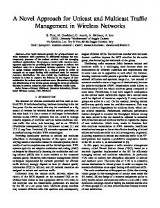
Fig. 2: Installation of a mobile Ad-Hoc network after an earthquake

5

Properties

In this section we use BUM to define and prove some properties of mobile ad hoc networks. First we review the properties for MANETs described in [11] and then we study some new properties which cannot be dealt with in the original CMN model. We use some examples to better describe the properties analyzed. We use a running example depicted in Figure 2, describing the case of an emergency due to an earthquake. The hospital sends tree ambulances to the emergency area (in figure A1, A2, A3). Then an ad hoc network is installed to manage the communication between the ambulances, placing a router near the epicenter of the earthquake. (in figure the orange circle). We have to make an assumption before starting to deal with the properties of BUM, about the possible receivers of the whole set of transmissions of a network. Given a process P , we denote by rcv(P ) the minimum set of locations ensuring that for each output action c¯L h˜ v i performed by P it holds that L ⊆ rcv(P ). Indeed, the tag L associated to an output action occurring in P can be either a variable or a set of locations, then we are not able to statically calculate rcv(P ). However. since an ad hoc network is usually designed to guarantee the communications within a specific area, we can reasonably assume that the underling protocol will always multicast messages to recipients located within the interested area and we can abstractly represent them by a finite set of locations. 5.1

Ubiquity of nodes

We now provide to demonstrate that the position of a node in the network has no effect on its behaviour. This characteristic allows us to consider movements, connections and disconnections of the nodes as weak actions, and give us insights on how to analyze the problem of Location Confidentiality, because a node can hide information about its location without modifying the process it is executing. This property is important especially in those cases where information confidentiality is important to protect: the best example is in case of war. In our example the ubiquity of nodes ensures that communication between 23

ambulances is not compromised by arbitrary movements of the nodes within the transmission cell of the router. Theorem 3 (Ubiquity of nodes). Let P be a process, λ1 , λ2 6= nil(l) locations of mobile nodes, k a location and r a transmission radius. Then: 1. n[P ]mλ1 ,r ≈ n[P ]mλ2 ,r 2. n[P ]sk,r ≈ n[P ]snil(k),r Proof. 1. We show that S S = {(n[P ]mλ1 ,r , n[P ]mλ2 ,r ) : ∀P, λ1 , λ2 6= nil(k), r} I is a bisimulation (where I is the identity relation). It is easy to prove because, if for some α we have α

n[P ]mλ1 ,r − → M, then, by applying rule (Move) if λ1 , λ2 6= nil, (m-Disc) or (m-Conn) otherwise, we obtain α ˆ

n[P ]mλ2 ,r =⇒ M . 2. We prove that S S = {(n[P ]sk,r , n[P ]snil(k),r ) : ∀P, k, r} I is a bisimulation (where I is the identity relation). Suppose, for any α α

n[P ]sk,r − → M, then, by applying (s-Conn) we obtain α ˆ

n[P ]snil(k),r =⇒ M . In the second case n[P ]snil(k),r can only log on, so τ

n[P ]snil(k),r − → n[P ]sk,r . 5.2

Silent nodes cannot be observed

What is interesting about the ad hoc networks are the interactions between nodes. If a node sends no messages, it does not interact with the network, then an external observer cannot know if this node is connected. Consider now the interactions between the hospital and the ambulances (Figure 3). Suppose that A1 and A2 are facing critical situations, and communicate with the hospital to prepare the acceptance of patients in hospital, while A3 have no patients to be accepted so no communications are sent from A3 to the hospital. The hospital broadcasts emergency messages to update the network about the general situation. An observer listening the communication between the nodes cannot know if A3 is connected, because it does not receive anything from that node. 24

Fig. 3: Messages exchange between H and the ambulances

Theorem 4 (Silent nodes are not observable). If the process P does not contain output constructs, then n[P ]µλ,r ≈ 0 ∀µ, λ, r. Proof. It follows from the definition of bisimilarity in which it is possible to match both τ -actions and input actions with weak τ -actions. 5.3

Obfuscating message transmission

We are going to propose a way to obfuscate messages transmission. This property is very important to reason about security problems and information and location confidentiality. We first have to prove that, alternating infinite output sequences, the order of the transmissions has got no effect to the behaviour of the node. We prove the theorem for a set of two messages (u and v), but the result can be generalized to an arbitrary set V = {v1 , ..., vn } of messages. Theorem 5 (Mixing up infinite output sequences). Let def

ALT (a, L1 , b, L2 ) = c¯L1 hai.¯ cL2 hbi.ALT ha, L1 , b, L2 i, then, for any n, r, u, v it holds that 1. n[ALT hu, L1 , v, L2 i]sσl ,r ≈ n[ALT hv, L2 , u, L1 i]sσ0 ,r , where σl , σl0 = l ∨ nil(l), l with l location. 2. n[ALT hu, L1 , v, L2 i]mλ1 ,r ≈ n[ALT hv, L2 , u, L1 i]mλ2 ,r , where λ1 , λ2 are locations or nil. Proof. 1. We prove that def

s S = {(n[ALT hu, L1 , v, L2 i]sσl ,r , n[ALT S hv, L2 , u, L1 i]σl ,r ) : 0 ∀r, u, v, σl , σl } I

is a bisimulation with respect to ≡. Since a node can connect or disconnect with weak actions, we directly consider connected devices, so σl , σl0 = l. Suppose 25

c!u@K

n[ALT hu, L1 , v, L2 i]sl,r −−−−→≡ n[ALT hv, L2 , u, L1 i]sl,r for some set K of locations, then, using (Lose) to discard v and (Obs) to transmit u, we obtain c!u@K

n[ALT hv, L2 , u, L1 i]sl,r =⇒ ≡ n[ALT hv, L2 , u, L1 i]sl,r With the same procedure we can show that, if c!v@K

n[ALT hv, L2 , u, L1 i]sl,r −−−−→≡ n[ALT hu, L1 , v, L2 i]sl,r , then: c!v@K

n[ALT hu, L1 , v, L2 i]sl,r =⇒ ≡ n[ALT hu, L1 , v, L2 i]sl,r . 2. We prove that def

m S = {(n[ALT hu, L1 , v, L2 i]mλ1 ,r , n[ALT S hv, L2 , u, L1 i]λ2 ,r ) : ∀r, u, v, λ1 , λ2 } I

is a bisimulation up to ≡. Suppose that c!u@K

n[ALT hu, L1 , v, L2 i]mλ1 ,r −−−−→≡ n[ALT hv, L2 , u, L1 i]mλ1 ,r for some set K of locations, then τ

n[ALT hv, L2 , u, L1 i]mλ2 ,r − → n[ALT hv, L2 , u, L1 i]mλ1 ,r by applying rule (Move), (m-Disc) or (m-Conn), in accordance with the value of λ1 and λ2 ; by applying (Lose) to discard v and (Obs) to transmit u, we deduce c!u@K

n[ALT hv, L2 , u, L1 i]mλ2 ,r =⇒ ≡ n[ALT hv, L2 , u, L1 i]mλ1 ,r . With the same procedure we can prove that, if c!v@K

n[ALT hv, L2 , u, L1 i]mλ2 ,r −−−−→≡ n[ALT hu, L1 , v, L2 i]mλ2 ,r , then: c!v@K

n[ALT hu, L1 , v, L2 i]mλ1 ,r =⇒ ≡ n[ALT hu, L1 , v, L2 i]mλ2 ,r . Now we have got all the notions to introduce a method to obfuscate messages transmission. A node m transmitting “ad infinitum” a message sequence, may obfuscate the transmission activity of nodes which are transmitting the same messages within the same transmission cell. this happens because nodes that receive a message cannot distinguish the sender, but only the channel of transmission. At a first analysis this property seems to be too much restrictive to be used in concrete situations, but there are many situations where packages transmitted in a network are standard. Consider the example of the network installed for the earthquake area: the ambulances and the hospital can 26

Fig. 4: Obfuscation of the transmission of v from the node n

communicate with standard messages. Consider for example the message v: “patient with cardiac arrest”, suppose that A1 transmits v “ad infinitum” to be sure that the hospital receives the message correctly. Then also A2 transmits the same package to the server, using the same channel: it could be result that the hospital prepares the acceptance for only one patient, but the patients with cardiac arrest are two. We choose this example to show how a deep analysis of these problems in transmission management are particularly important in mobile ad hoc networks, because this kind of network is used in critical situations. In our example message obfuscation results to be an obstacle for the good management of networks, a problem rather then a property. In other cases we can prove that the possibility of a node to hide its transmission could be a positive future (as in case of war). A formal model as BUM, has the purpose of analyzing deeply the characteristics of the networks, with both their positive and negative consequences for the communication management.

Fig. 5: Example of obfuscation in transmission of v by A1

27

Theorem 6 (Obfuscating message transmission). Let P and Q be two processes such that f c(P, Q) ⊆ {c} for some channel c, where all the output actions of P and Q are in the set {¯ cL1 hui, c¯L2 hvi}. Then: 1. n[P ]sσk ,r |m[ALT hu, L1 , v, L2 i]sσk ,r ≈ n[Q]sσk ,r |m[ALT hu, L1 , v, L2 i]sσk ,r , where σk = k ∨ nil(k) 2. n[P ]mλ1 ,r |m[ALT hu, L1 , v, L2 i]mλ2 ,r ≈ n[Q]mλ3 ,r |m[ALT hu, L1 , v, L2 i]mλ4 ,r , where λi 6= nil(k)∀1 ≤ i ≤ 4 for any location k. Proof. 1. As ≈ is transitive, We have only to show n[P ]sσk ,r |m[ALT hu, L1 , v, L2 i]sσk ,r ≈ m[ALT hu, L1 , v, L2 i]sσk ,r because we will use the same procedure to prove that n[Q]sσk ,r |m[ALT hu, L1 , v, L2 i]sσk ,r ≈ m[ALT hu, L1 , v, L2 i]sσk ,r then we can deduce n[P ]sσk ,r |m[ALT hu, L1 , v, L2 i]sσk ,r ≈ m[ALT hu, L1 , v, L2 i]sσk ,r ≈ n[Q]sσk ,r |m[ALT hu, L1 , v, L2 i]sσk ,r . Since the nodes can disconnect an connect arbitrarily in the network simply executing weak actions, we can directly consider the case in which n and m are connected, so σk = k. We then prove the relation S = {(n[P ]sk,r |m[ALT hu, vi]sk,r , m[ALT hu, vi]sk,r ) : ∀u, v, k, r, ∀P.f c(P ) ⊆ {c} where all output actions of P are S {¯ cL1 hui, c¯L2 hvi}} I is a bisimulation up to≡. Suppose then c!u@K

n[P ]sk,r |m[ALT hu, vi]sk,r −−−−→≡ M for some set K of nodes. if m is the sender of u we have M ≡ n[P ]sk,r |m[ALT hv, ui]sk,r . If n is the sender of message we have M ≡ n[P 0 ]sk,r |m[ALT hu, vi]sk,r , c!u@K

where n[P ]sk,r −−−−→ n[P 0 ]sk,r . In the first case it simply suffices an application of (Obs) also to m[ALT hu, vi]sk,r , obtaining m[ALT hv, ui]sk,r , whereas in the second case, after an application of (Obs) we use (Lose) to discard v obtaining m[ALT hu, vi]sk,r again. it is easy now to prove that (n[P ]sk,r |m[ALT hv, ui]sk,r , m[ALT hv, ui]sk,r ) and 28

(n[P 0 ]sk,r |m[ALT hu, vi]sk,r , m[ALT hu, vi]sk,r ) are members of S, because the same properties of the initial couple are still valid (f c(P 0 ) ⊆ {c} and all output actions of P 0 are {¯ cL1 hui, c¯L2 hvi}), so it suffices the application of the same procedure. 2. As ≈ is transitive, it suffices proving n[P ]mλ1 ,r |m[ALT hu, vi]mλ2 ,r ≈ m[ALT hu, vi]mλ,r , because we then use the same procedure to demonstrate n[Q]mλ3 ,r |m[ALT hu, vi]mλ4 ,r ≈ m[ALT hu, vi]mλ,r , we then deduce n[P ]mλ1 ,r |m[ALT hu, vi]mλ2 ,r ≈ m[ALT hu, vi]mλ,r ≈ n[Q]mλ3 ,r |m[ALT hu, vi]mλ4 ,r . We now prove that the relation S = {(n[P ]mλ1 ,r |m[ALT hu, vi]mλ2 ,r , m[ALT hu, vi]mλ,r ) : ∀u, v, λ, λ1 , λ2 , r, ∀P.f c(P ) ⊆ {c} where all output actions of P are S {¯ cL1 hui, c¯L2 hvi}} I is a bisimulation up to ≡. Suppose c!u@K

n[P ]mλ1 ,r |m[ALT hu, vi]mλ2 ,r −−−−→≡ M . if m is the sender of u, we have M ≡ n[P ]mλ1 ,r |m[ALT hv, ui]mλ2 ,r , if n is the sender of the message we have M ≡ n[P 0 ]mλ1 ,r |m[ALT hu, vi]mλ2 ,r , c!u@K

where n[P ]mλ1 ,r −−−−→ n[P 0 ]mλ1 ,r . In both cases we use the rule (Move) ((mτ Disc) if λ2 = nil, (m-Conn) if λ = nil) and we obtain m[ALT hu, vi]mλ,r − → m m[ALT hu, vi]λ2 ,r . Then, in the first case it simply suffices an application of rule (Obs) also to m[ALT hu, vi]mλ2 ,r obtaining m[ALT hv, ui]mλ2 ,r , in the second case, after an application of rule (Obs) we use (Lose) to discard v obtaining m[ALT hu, vi]mλ2 ,r again. it is is easy now to prove that (n[P ]mλ1 ,r |m[ALT hv, ui]mλ2 ,r , m[ALT hv, ui]mλ2 ,r ) and (n[P 0 ]mλ1 ,r |m[ALT hu, vi]mλ2 ,r , m[ALT hu, vi]mλ2 ,r ) are in S because the same properties of the initial couple are still valid (f c(P ) ⊆ {c} where all output actions of P are {¯ cL1 hui, c¯L2 hvi}), so it suffices applying the same procedure. 29

Fig. 6: Radii of maximum observability

5.4

Radius of maximum observability

All the properties described above can be proved also in the original CMN [11]; now we introduce new properties which cannot be dealt with in CMN. The first important characteristic we are going to describe is about the transmission radius of the nodes. Each transmission is associated to a set of locations including the receivers of the message. Then we can define a “radius of maximum observability”, that is a radius such to allow a correct reception of a message to all the locations of the receivers set. In particular we can define the “minimum radius of maximum observability”, which corresponds to the distance between the sender of the message and the most distant receiver. Figure 6 illustrates three different cases of a transmission effect in a network: the black radius (the smallest) does not allow the reception of the message by the set of the receivers (light nodes) while the other two radii reach at least one of the receivers. The orange radius is in particular the distance between the transmitter and the most distant receiver: This characteristic means that this is the minimum radius of maximum observability. To understand how this property is important let consider the example depicted in Figure 7. The earthquake has damaged a defined area; we can than deduce that rescuers need to communicate only within the emergency area (in figure the area delimited by the orange circle). We can then determine the minimum transmission radius which ensures the central server of the hospital to be able to communicate with the ambulances sent for assistance in the disaster area. This property is important only for stationary nodes, whereas a mobile node can move within the transmission cell of the transmitter to receive the communication. In our example the central server needs to communicate with the ambulances, which are all mobile nodes, then instead of determining the minimum radius of maximum observability, which change arbitrarily, it is better considering a radius enough large to ensure the correct result of the transmission within all the emergency area. Although we can define a minimum radius to reach all the intended receivers of a transmission, we cannot be sure of the correct reception of the message 30

Fig. 7: determination of the minimum radius of maximum observability

by the whole set of intended receivers; There are indeed various obstacles (as connection failures, ore physical barriers to transmissions...) which can obstruct the correct outcome of a transmission in the network; This is the reason why the output actions are always observable, while the input actions are not. Theorem 7 (Radius of maximum observability). Let P be a process such that rcv(P ) = L, if, for some r, σl = l ∨ σl = nil(l), d(l, k) 6 r ∀k ∈ L, then: n[P ]sσ0 ,r0 ≈ n[P ]sσl ,r ∀r0 ≥ r and ∀σl0 = l ∨ σl0 = nil(l). l

In this case we say that r is a radius of maximum observability for the stationary process P located at σl . Proof. We prove that the relation S = {(n[P ]sσl ,r , n[P ]sσ0 ,r0 ) : l ∀r0 ≥ r, ∀σl , σl0 =Sl ∨ nil(l), ∀P.rcv(P ) = L} I is a bisimulation. Consider c!v@L

i n[P ]sσl ,r −−−−→ n[P 0 ]sσl ,r , with Li ⊆ L.

cL !v[l,r]

i Then, by applying rule (Obs) backward it must be Then we have n[P ]sσl ,r −−− −−−→ 0 s n[P ]σl ,r , as d(l, li ) ≤ r∀li ∈ Li ⊆ L, and by applying rule (Snd) backward we

c¯L v

i finally obtain P −−− → P 0 . So we can write

c!v@K

n[P ]sσ0 ,r0 =⇒ n[P 0 ]sσl ,r0 l

where K = {k : k ∈ Li ∧ d(l, k) ≤ r0 }. Then Li ⊆ K because, if d(l, k) ≤ r necessarily d(l, k) ≤ r0 , recalling that r ≤ r0 ; We can also write K ⊆ Li by definition of K, then K = L, and we deduce 31

c!v@L

n[P ]sσl ,r0 =⇒ i n[P 0 ]sσl ,r0 Now it is sufficient to prove that n[P 0 ]sσl ,r Sn[P 0 ]sσl ,r0 We know that for P 0 the same properties of P are valid (rcv(P 0 ) ⊆ L for definition of the function rcv(·)), we can then apply to P 0 the same procedure used for P . Definition 7 (Minimum Radius of Maximum observability). Let consider a process P such that rcv(P ) = L, we say that r is the minimum radius of maximum observability for the stationary node P located at σl if r is a radius of maximum observability, and if for all r0 < r it holds that r0 is not a radius of maximum observability for the stationary node P located at σl . 5.5

Simulation of stationary nodes in different locations

Fig. 8: Example of simulation of stationary nodes in different locations

The tag L associated to each output action has been introduced, not only in order to find the minimum radius ensuring each transmission to reach all its receivers, but its introduction allows us to define other important properties for our calculus. If we pay attention to the behaviour of stationary nodes, we realize that the tag L enables, under particular prerequisites, the simulation of stationary devices in different locations. In our calculus the barb of a transmission is not determined by a set of locations, but by the intersection of two sets: more precisely the barb of a transmission is given by the set of locations which are members of L, lying in the transmission cell of the sender. By these assumptions, we can now consider the case where two stationary nodes, placed in different locations (with therefore different neighbours), but communicating with the same set of locations, result to have the same barb. A practical example of the usefulness of this property is the case we have to use the lowest number of routers within an area in order to ensure the communication with a 32

Fig. 9: Example of optimizing routers allocation

r1

r3

r2

r4

Generic nodes Receivers

Generic nodes Receivers

Routers  

 

Routers

Transmission radius of routers

 

(a) initial network topology

r1

r3

r2

r4

Routers  

Transmission radius of routers

(b) First routers allocation

Generic nodes Receivers

 

 

Transmission radius of routers

(c) Optimal routers allocation

33

given set of locations. If we realise that two different routers result to have the same behaviour, one of them can be then turn off, allowing us to save power and physical resources. Looking at Figure 9 we can see an example of optimizing the allocation of the routers, by turning off the router r3, which is not usefull, because it can be simulated by r1. Theorem 8 (Simulation of stationary nodes in different locations). Let P be a process with rcv(P ) = L. Suppose: n[P ]sσl ,r with σl = l ∨ nil(l) and K = {k : k ∈ L ∧ d(l, k) ≤ r} m[P ]sσl0 ,r0 with σl0 = l0 ∨ nil(l0 ) and K 0 = {k 0 : k 0 ∈ L ∧ d(l0 , k 0 ) ≤ r0 }. It holds that: 1. If K 0 ⊆ K, then n[P ]sσl ,r simulates m[P ]sσl0 ,r0 ; 2. If K = K 0 , then n[P ]sσl ,r ≈ m[P ]sσl0 ,r0 . Proof. 1. the interesting case to analyse is the output action. Consider P = c¯Li hvi.P 0 for some Li ⊆ L: c!v@K 00

m[P ]sσl0 ,r0 −−−−−→ m[P 0 ]sσl0 ,r0 , where K 00 = K 0 ∩ Li Then we can write n[P ]sσl ,r

c!v@K 000

=⇒ n[P 0 ]sσl ,r where K 000 = K ∩ Li .

But, as K 0 ⊆ K, we deduce K 0 ∩ Li = K 00 ⊆ K 000 = K ∩ Li and, by applying rules (Obs) we can also write c!v@K 00

n[P ]sσl ,r =⇒ n[P 0 ]sσl ,r . As rcv(P 0 ) ⊆ L, by applying the same procedures to P 0 we can prove that n[P 0 ]sσl ,r simulates m[P 0 ]sσl0 ,r0 . 2. If K = K 0 then K ⊆ K 0 and K 0 ⊆ K; so, by applying the same procedure used to prove the first item of this theorem, we demonstrate that the relation S = {(n[P ]sσl ,r , m[P ]sσl0 ,r0 ) : 0 0 ∀σl = l ∨ nil(l), ∀σ Sl0 = l ∨ nil(l ) ∀P.rcv(P ) ⊆ L} I is a bisimulation. 5.6

Range repeaters

We are going to define the Range Repeaters, that are devices which regenerate a network signal in order to extend the range of the existing network infrastructure. A definition of repeater was already given in [11]. Here we give a new definition of range repeater for BUM, and we use both range repeaters with one and two channels to prove new important properties. 34

Definition 8. Let a, b be channels, l a location, r a transmission radius and L a set of locations. A repeater with two channels on L is a stationary device, denoted rr[a ,→L b]sl,r , where a ,→L b is a process whose general recursive definition is: def a ,→L b = a(x).¯bL hxi.a ,→L b.

A range repeater with two channels receive values through the input channel and retransmits them through the output channels, to the message receivers. A range repeater with one channel operates analogously, but input and output channels coincide. Definition 9. Let c be a channel, l a location, r a transmission radius and L a set of locations. A range repeater with one channel on L is a stationary device, denoted rr[c ,→L c]sl,r .

Fig. 10: Range repeater with one channel

(a) n[P ]sk,r

(b) n[P ]sk,r0 |rr[c ,→L c]sl,r

Range repeaters are usually exploited to enlarge transmission cell of a stationary node and, if such a node always communicates with the same set of devices, each time through the same channel, by using a range repeater we can simulate the presence of the sender in the location of the repeater. The employment of range repeaters is particularly interesting for Ad-Hoc Networks, because it allows us to analyze and try to solve the problems of devices mobility. Consider once more the example used in this section. Describing the situation we did not consider distance between the hospital and the earthquake area, which may be too large to guarantee the communication with the ambulances running up in the emergency area. It will be then necessary employing a range repeater enough powerfull to cover all the area and, at the same time, reachable by the central server of the hospital. If the earthquake epicenter is too distance from the hospital we can install a series of consecutive repeaters, which will connect the central server to the disaster area. 35

Fig. 11: Example of repeaters use

Theorem 9 (Range repeaters with one channel). Let P be a process such that f c(P ) ⊆ {c} for some channel c. Let rcv(P ) = L. Let k, l be physical locations, r, and r0 radii such that d(k, l) ≤ r and d(k, l) ≤ r0 . Then: n[P ]sk,r0 |rr[c ,→L c]sl,r simulates n[P ]sl,r . Proof. We have to prove that the relation def

S = {(n[P ]sl,r , n[P ]sk,r0 |rr[c ,→L c]sl,r ) : ∀l, k, r, r0 .d(k, l) ≤ r ∧ d(l, k) ≤ r0 ∀P.f c(P ) ⊆ {c} ∧ rcv(P ) = L} is a simulation. Suppose: c!v@K

n[P ]sl,r −−−−→ n[P 0 ]sl,r c¯L v

i for K = {k1 , ..., kn : ki ∈ Li ∧ d(l, ki ) ≤ r ∀ 1 ≤ i ≤ n}, because P −−− → P 0 for 0 some Li ⊆ L. Knowing that d(k, l) ≤ r , by applying rule (Bcast) we obtain:

cL !v[k,r 0 ]

n[P ]sk,r0 |rr[c ,→L c]sl,r −−i−−−−→ n[P 0 ]sk,r0 |rr[¯ cL hvi.c ,→L c]sl,r , and, by applying rule (Obs), c!v@K 0

n[P 0 ]sk,r0 |rr[¯ cL hvi.c ,→L c]sl,r −−−−−→ n[P 0 ]sk,r |rr[c ,→L c]sl,r , where 0 K = {k10 , ..., kn0 : ki0 ∈ L ∧ d(l, ki0 ) ≤ r ∀ 1 ≤ i ≤ n} that means: c!v@K 0

n[P ]sk,r0 |rr[c ,→L c]sl,r =⇒ n[P 0 ]sk,r |rr[c ,→L c]sl,r But, as Li ⊆ L then K ⊆ K 0 , by using rule (Lose) to hide the communications with nodes at locations in K 0 which are not in K we can finally write: c!v@K

n[P ]sk,r0 |rr[c ,→L c]sl,r =⇒ n[P 0 ]sk,r |rr[c ,→L c]sl,r 36

We have now only to prove that (n[P 0 ]sl,r , n[P 0 ]sk,r0 |rr[c ,→L c]sl,r ) ∈ S Since for P 0 the same properties of P are still valid (f c(P 0 ) ⊆ {c} ∧ rcv(P 0 ) ⊆ L) we can apply the same procedure and prove in this way the simulation. We are going now to prove that the simulation just described can be realized also with a range repeater with two channels. Using two channels however we need two range repeaters, respectively for input (in[d ,→L c]sl,r ) and output (out[c ,→L d]sl,r ) management. The diagram in figure 12 illustrates the employment of the channels and the interaction between the nodes in the realization of range repeaters with one or two channels. This figure is inspired to the diagrams of Milner [13] in his introduction to CCS, describing the behaviour of agents and the use of channels for data input and output. We emphasise that this kind of diagrams gives no information about physical position of nodes or about network topology, but it only shows the connections through which devices can exchange data.

Fig. 12: Range repeaters: diagram of the interaction between the nodes

(a) rr[c ,→L c]sl,r

(b) in[d ,→L c]sl,r |n[P ]sk,r0 |out[c ,→L d]sl,r

Theorem 10 (Range repeaters with two channels). Let P be a process such that f c(P ) ⊆ {c} and rcv(P ) = L, let l and k be physical locations, r, r0 transmission radii such that d(k, l) ≤ r and d(l, k) ≤ r0 . Then, for any channel d: n[P ]sk,r0 |out[c ,→L d]sl,r |in[d ,→L c]sl,r simulates n[{d/c}P ]sl,r . Proof. Proof is given with the same method used for the previous theorem, so we prove that the relation def

S = {(n[{d/c}P ]sl,r , n[P ]sk,r0 |out[c ,→L d]sl,r |in[d ,→L c]sl,r ) : ∀l, k, r, r0 .d(k, l) ≤ r ∧ d(l, k) ≤ r0 ∀P.f c(P ) ⊆ {c} ∧ rcv(P ) = L} 37

is a simulation. Suppose: d!v@K

n[{d/c}P ]sl,r −−−−→ n[{d/c}P 0 ]sl,r c¯L v

i for K = {k1 , ..., kn : ki ∈ Li ∧ d(l, ki ) ≤ r ∀ 1 ≤ i ≤ n} because P −−− → P 0 for 0 some Li ⊆ L. knowing that d(k, l) ≤ r , by applying rule (Bcast) we obtain

cL !v[k,r 0 ]

n[P ]sk,r0 |out[c ,→L d]sl,r |in[d ,→L c]sl,r −−i−−−−→ n[P 0 ]sk,r0 |out[d¯L hvi.c ,→L d]sl,r |in[d ,→L c]sl,r . Now we can exploit the repeater out, created on purpose for output actions. By applying firs rule (Bcast) and later rule (Obs) we obtain: d!v@K n[P 0 ]sk,r0 |out[d¯L hvi.c ,→L d]sl,r |in[d ,→L c]sl,r =⇒ n[P 0 ]sk,r0 |out[c ,→L d]sl,r |in[d ,→L c]sl,r

0

0 with K 0 = {k10 , ..., km : ki0 ∈ L ∧ d(l, ki0 ) ≤ r ∀ 1 ≤ i ≤ m}. Then: d!v@K 0

n[P ]sk,r0 |out[c ,→L d]sl,r |in[d ,→L c]sl,r =⇒ n[P 0 ]sk,r0 |out[c ,→L d]sl,r |in[d ,→L c]sl,r .

As Li ⊆ L we deduce that also K ⊆ K 0 and, by applying rule (Lose) to all the nodes with locations in K 0 which are not in K we can also write: d!v@K

n[P ]sk,r0 |out[c ,→L d]sl,r |in[d ,→L c]sl,r =⇒ n[P 0 ]sk,r0 |out[c ,→L d]sl,r |in[d ,→L c]sl,r Now it is sufficient to prove that

(n[P 0 ]sl,r , n[P 0 ]sk,r0 |out[c ,→L d]sl,r |in[d ,→L c]sl,r ) ∈ S Since for P 0 the same properties of P are still valid (f c(P 0 ) ⊆ {c}∧rcv(P 0 ) ⊆ L), by applying the same procedure used for P we can prove the simulation. Suppose now that an input action is executed, then we use in. Suppose: d?v@l

n[{d/c}P ]sl,r −−−−→ n[{d/c}{v/x}P 0 ]sl,r cv

because P −→ {v/x}P 0 . Since it lies in location l, also in can receive v through channel d. In particular we have: d?v@l

n[P ]sk,r0 |out[c ,→L d]sl,r |in[d ,→L c]sl,r −−−−→ n[P ]sk,r0 |out[c ,→L d]sl,r |in[¯ cL hvi.d ,→L c]sl,r Now, by applying rule (Bcast), recalling that P = c(x).P 0 , we can write: cL !v[l,r]

n[P ]sk,r0 |out[c ,→L d]sl,r |in[¯ cL hvi.d ,→L c]sl,r −−−−−→ 0 s n[{v/x}P ]k,r0 |out[c ,→L d]sl,r |in[d ,→L c]sl,r We can then deduce: d?v@l

n[P ]sk,r0 |out[c ,→L d]sl,r |in[d ,→L c]sl,r =⇒ n[{v/x}P 0 ]sk,r0 |out[c ,→L d]sl,r |in[d ,→L c]sl,r 38

Now it is sufficient to prove that (n[{v/x}P 0 ]sl,r , n[{v/x}P 0 ]sk,r0 |out[c ,→L d]sl,r |in[d ,→L c]sl,r ) ∈ S Since for P 0 the same properties of P are still valid (f c(P 0 ) ⊆ {c}∧rcv(P 0 ) ⊆ L), by applying the same procedure we can finally prove the simulation. Defining the Minimum Radius of Maximum Observability, we have emphasised the importance of ensuring that a message transmission can reach the whole set of intended receivers. By applying this concept to the definition of range repeater, we can introduce the notion of complete range repeater, that is a repeater which has a radius enough large to reach all the locations in the set of receivers. Definition 10 (Complete range repeater). We define the repeater complete on L as a repeater rc[c ,→L c]sl,r whose barb coincides with L, i.e., rc[c ,→L c]sσl ,r ⇓c and d(l, k) 6 r∀k ∈ L. Looking at the example in Figure 11, where we suppose that a repeater is installed to allow the central server of the hospital to communicate with the ambulances, we can notice how the repeater has been chosen such as to guarantee that its transmission radius (the red segment in figure) covers the complete area of the disaster (orange line in figure). This is also an example of a complete range repeater, whose radius is a radius of maximum observability for the entire earthquake area. The use of a complete range repeater reduces the problem of ensuring the communication between the central server and a set of locations, to the communication between only two devices: H will be then sure that, in whatever locations the ambulances will lie, they will be always reachable by rr. Theorem 11 (Complete range repeaters). Let c be a channel, l and k locations (in particular σk = k ∨ nil(k) and σl = l ∨ nil(l)), r and r0 be transmission radii. Let P be a process such that f c(P ) ⊆ {c} and rcv(P ) = L. Finally let rc[c ,→L c]sσl ,r be a complete range repeater on L, lying at location l, with radius r. Then: n[P ]sσk ,r0 |rc[c ,→L c]sσl ,r ⇓c ∀k, r0 .d(k, l) ≤ r0 , and all the recipients of L will be reachable by the node n. It means that, for each fragment of the process P executing an output action c¯Li hvi i.Q such that P = P 0 .¯ cLi hvi i.Q it holds c!v@L

i n[¯ cLi hvi i.Q]sσk ,r0 |rc[c ,→L c]sσl ,r −−−−→ n[Q]sσk ,r0 |rc[c ,→L c]sσl ,r

Proof. Let consider P = P1 .¯ cL1 hv1 i.Q, and c¯L1 hv1 i is the first output action in τ process P ( we can write P =⇒ c¯L1 hv1 i.Q). We can write n[P ]sσk ,r0

cL1 !v1 [k,r 0 ]

=⇒

n[Q]sσk ,r0

since d(l, k) ≤ r0 we have n[P ]sσk ,r0 |rc[c ,→L c]sσl ,r

cL1 !v1 [k,r 0 ]

=⇒

By applying rule (Bcast) we can write 39

n[P 0 ]sσk ,r0 |rc[¯ cL hvi.c ,→L c]sσl ,r

cL !v1 [l,r]

n[P 0 ]sσk ,r0 |rc[¯ cL hvi.c ,→L c]sσl ,r −−−−−−→ n[P 0 ]sσk ,r0 |rc[c ,→L c]sσl ,r By applying rule (Obs), knowing that L1 ⊆ L and consequently d(l, k) ≤ r ∀k ∈ L1 we can write n[P ]sσk ,r0 |rc[c ,→L c]sσl ,r

c!v1 @L1

=⇒ n[P 0 ]sσk ,r0 |rc[c ,→L c]sσl ,r

By our definition of Barb, using Harmony theorem we can deduce also n[P ]sσk ,r0 |rc[c ,→L c]sσl ,r ⇓c and the set of receivers is L because d(k, l) ≤ r ∀k ∈ L. For the successive output actions of the process P the proof is similar because we know that each Li ⊆ L is completely reachable by the range repeater used. 5.7

The problem of Interference

Fig. 13: Example of Interference: a node with a too large transmission energy may disturb the other transmission within the network

Node interfering with the network Transmission radius

One of the most critical problems in managing an ad hoc network is the power consumption, since it can be constituted of different kinds of nodes which may be powered with weak battery. The concept of topology control is the technique used in order to reduce the initial topology of the network to save energy and to extend the lifetime of the network. This can be then considered as a tradeoff between power saving and network connectivity. In other words when we have to choose the transmission power of each node, we know that choosing a low transmission power for a node we will reduce its connectivity within the network, but we also reduce its power consumption. The main goal of topology control is therefore the choice, for each node, of a minimum transmission power which guarantees network connectivity. There is an other problem depending on the transmission power we chose for a node sending data within the network: a too large transmission radius will reach a large number of nodes, and there is a higher probability to disturb devices not interested in receiving the data transmitted, and to congest the network. 40

Following the definition of interference introduced in [5], the notion of interference arises from a natural question: How many other nodes a given network node can disturb? Consider a node transmitting a message, we can then define the interference as the number of nodes listening to the message, but not interested in receiving it. Definition 11 (Interference). Let consider an output action cL !˜ v [l, r], and K = {k : d(l, k) ≤ r}, then the level of interference with respect to this output is defined as: I(cL !˜ v [l, r]) = |K − L| For example, looking at Figure 13 we can observe that the red node has got a transmission radius large enough to reach all the nodes of the network: this is not a positive characteristic because means a large energy consumption, together with a higher probability of collisions with other transmission and a consequent network congestion. Once we have explained the notion of interference, given a transmission, if the set of nodes not interested in receiving the transmission is empty, we can affirm that there is not interference in the communication , i.e. if I(cL !˜ v [l, r]) = 0, then we say that there is no interference in the communication. Using BUM in order to describe the case in which a transmission reaches only the receivers, without any “interference” we can compare the behaviour of a node communicating with a given set L of recipients, with the same node broadcasting the same communication to the whole network. If what results from this comparison is a bisimulation, this means that there is no interference in the transmission considered, in other words this action will not “disturb” any other node of the network. Let us first define the broadcasting version of a process P , denoted by brd(P ), as follows: – – – –

if if if if

P P P P

= 0 then brd(P ) = 0; = c(˜ x).P 0 then brd(P ) = c(˜ x).brd(P 0 ); 0 = c¯L h˜ v i.P then brd(P ) = c¯∞ h˜ v i.brd(P 0 ). = [w1 = w2 ]Q, R then brd(P ) = [w1 = w2 ]brd(Q), brd(R).

Definition 12 (Interference-freeness). We say that a node n[P ]µl,r is interferencefree whenever µ n[P ]µl,r ∼ = n[brd(P )]l,r .

Theorem 12. If n[P ]µl,r is interference-free then for all output actions cL !˜ v [l, r] µ performed by n[P ]l,r it holds that I(cL !˜ v [l, r]) = ∅. Proof. We will give a proof by contradiction. Since n[P ]µl,r is interference-free we can write: µ n[P ]µl,r ∼ = n[brd(P )]l,r

41

cL !v[l,r]

Let consider a derivative n[P 0 ]µl0 ,r of n[P ]µl,r such that n[P 0 ]µl0 ,r −−−−−→ n[P 00 ]µl0 ,r . µ µ µ Since n[P ]µl,r ∼ = n[brd(P )]l,r there exists a derivative n[Q0 ]l00 ,r of n[brd(P )]l,r such µ 0 µ 0 0 that n[P ]l0 ,r ∼ = n[Q ]l00 ,r . Now suppose by contradiction that I(cL !v[l , r]) > 0. Then, by definition of Interference it holds that there exists k such that d(l0 , k) ≤ r and k ∈ / L. If we apply rule (Obs) to n[Q0 ]µl00 ,r , assuming that only k could receive v˜, then we will write: c!˜ v @k

n[Q0 ]µl00 ,r −−−−→ n[Q00 ]µl00 ,r But we cannot write: c!˜ v @k

n[P 0 ]µl0 ,r =⇒ n[P 00 ]µl0 ,r µ because k ∈ / L. Since we assumed that n[P 0 ]µl0 ,r ∼ = n[Q0 ]l00 ,r , we reached a contradiction.

6 6.1

An example of BUM employment: the AODV Routing protocols for mobile ad hoc networks

One of the most critical problems in the development of a mobile ad hoc network is the packets routing. When choosing the routing protocol we have to pay particular attention to the operational cost, since devices may be power limited (ad hoc networks are often composed of notebooks, mobile phones...); we have also to consider that there can be cases of non-cooperation of two types of nodes: selfish ones that want to save power, and malicious nodes that are interested in attacking the network. We can classify routing protocols in three different categories: – Proactive protocols: this kind of protocol maintain a list of destinations with the routes to reach them, and periodically refresh it. The advantage of these protocols is that every time a node wants to communicate with some other device, it has got the information it needs immediately; otherwise there are disadvantage due to the cost of data freshness maintaining. – Reactive protocols: this kind of protocol find a route only on demand. The advantage that protocol search only the useful data, otherwise, when a node send a request, there can be a high latency time for the response to be received. – Hybrid routing: there are some routing protocols that combine both reactive and proactive routing (in hierarchical protocols for example the choice of using a reactive or a proactive routing depends on the hierarchical level of a node looking for a route). One of the most used routing protocols in a MANET’s implementation is the AODV (Ad hoc On-demand Distance Vector Routing) [6], [21], [1], [23], which has been chosen to illustrate the usefulness of our calculus, just because of its common employment in this kind of situations. 42

The AODV is a reactive protocol which provides the best routes between the nodes only by request, and uses a set of sequence numbers to guarantee received data to be always updated. The older CMN appeared unsuitable to represent this protocol, because it supports only broadcast communication, while the AODV needs also unicast and multicast transmissions. The main packets of this protocol are three: RREQ (route request), that is usually transmitted via broadcast, RREP (route reply), that is instead transmitted to the requester with an unicast transmission, and RERR (packet transmitted by a node after a connection failure); the best kind of transmission for RERR packets is the multicast communication, because not all the nodes of the network are interested in receiving this information, but only the devices that need to refresh their route table. Figure 14 describes the behavior of RREQ and RREP propagation: notice that a request broadcast generates an explosion of messages (Figure 14.a), while the reply, using a unicast communication, will be propagated to a limited number of locations (Figure 14.b). AODV is one of the most used protocols for mobile ad hoc networks, otherwise there are also other protocols used in this kind of contexts. For example in some cases we can find the proactive version of the AODV, that is DSDV (Destination-Sequenced Distance Vector routing) [16], that uses the same technique of its reactive version, but it finds all possible routes within the network regardless of the fact that they will be useful or not; An other used reactive protocol for MANETs is DSR (Dynamic Source Routing) [18], which is similar to AODV, but it uses source routing instead of relying on the routing table at each intermediate device; as concerns the hybrid protocols we can find for example ZRP (Zone Routing Protocol) [10] or GSR (Global State Routing) [7] which in particular is a hierarchical routing protocol which is based on link state vectors (nodes exchange vectors of link states among their neighbors during routing information exchange). In this section we are going to give an implementation of AODV to show the usefulness of our calculus for the analysis of concretes problems in the implementation of a mobile ad hoc network. Even though we consider only one of a great number of possible choices for the routes management, since the most routing protocols used in mobile ad hoc networks implementations have some common characteristics, we are persuaded that even changing the routing protocol, this calculus could be anyway able to capture properties and problems in the network management. 6.2

Details of the algorithm

Each node maintains tables to store information about its neighbors. In particular a route table is associated to each node, with an IP address k as key. it contains the following information: – seq#k denotes the sequence number of the node k; – nexthop denotes the address of the first node in the route from the source to k; 43

Fig. 14: Example of route request and reply from S to D

(a) RREQ broadcast

(b) RREP transmission

– hopcount denotes the number of steps which separate the source from k; – lifetime denotes the validity of the record in the table; – List of precursors denotes the list of nodes that use the source as the nexthop towards the destination. The protocol manages route requests to connect the nodes of the network through the three packets mentioned before; more precisely: RREQ (Route Request): A node looking for a route broadcasts an RREQ packet (Figure 14.a), then waits. It will choose the best route (in terms of costs, of reply time, or route length). RREP (Route Response): A node receiving an RREQ makes a first control to verify if it is an intended recipient of the message, if the condition is verified it immediately replies, otherwise it looks in its route table if there exists a valid route for that destination; finally, if it has got no information to generate the RREP, it propagates the RREQ before answering (Figure 14.b). RERR (Route Error): the error message is used for warning the network that a node is no more reachable (this situation happens for several reasons, as the disconnection of a node, or a software/hardware damage) As we just told about before, a “sequence number”(seq#l ) has been associated to each node; it has been increased every time that a node decides to broadcast an RREQ, or a node that receives an RREQ, and that is exactly the destination of the route request, have to send back the reply. In this second case the sequence number to be increased will be chosen between the current value and the value written in the RREQ packet. RREQ in detail As Figure 15 illustrates, a packet RREQ contains: 44

Fig. 15: RREQ packet structure

– the field Bid (Broadcast ID), which identifies the packet; it is incremented every time a new copy of the same request is broadcasted; – The couple (s, seq#s ), denoting the IP address and the sequence number of the route source; – The couple (d, seq#d ), denoting the IP address and the sequence number of the route destination; – The field hopcount, initialized to zero; – The field lifetime, denoting the validity of the information contained in the packet. Each time a node sends a request, it waits the reply and then refreshes its route table with the new information acquired. A node after having received an RREQ: 1. Controls if the received RREQ is a new information or a duplicate; 2. If the node itself is the destination of the request it immediately sends back the reply; 3. Otherwise controls the information contained in the route table. If it has got the required information, and the sequence number of the destination is at least the same of the request sequence number, it immediately answers with an RREP packet; 4. If the entries of its route table are too old, it increments Bid and hopcount, propagates the request and, once the reply is received, it sends back to the source the RREP required. The field hopcount is necessary for the creation of a Reverse route, that is an entry in the route table of the node having received the request, made using the information contained in the RREQ, modelling a path from the current node to the source of the RREQ transmission. Notice that Bid is a progressive number increased each time a request is transmitted again; this field is necessary for the good operating of the protocol, because it prevents the network from loops in RREQ propagations. Figure 16 emphasizes the importance of using a Broadcast ID in a route request. In particular we show what can happen by omitting this field in the 45

Fig. 16: Loop caused by an RREQ transmission without duplicates control

RREQ: a node could receive continuously the same packet without recognizing it, and repropagates it “ad infinitum”. There can be generated loops, causing network obstruction and power dissipation. RREP in detail

Fig. 17: RREP packet structure

As Figure 17 illustrates, RREP packet contains: – – – –

The The The The

couple (s, seq#s ), with the sequence number updated; couple (d, seq#d ), with the sequence number updated; field hopcount with the number of the steps needed by s to reach d; field “lifetime” updated.

As we just told in describing RREQ packet, a node answers with an RREP when it is itself the destination or when it has got the required information updated. If the node is the destination of the request: 46

1. if the RREQ sequence number is greater then the one of the node having received the packet, the receiver updates its sequence number with the RREQ’s one, then it increments it. 2. it builds and broadcasts the RREP with the new sequence number of the destination, and hopcount incremented. If the node having received the RREQ is not the destination, but it has got the required information: 1. it updates the field hopcount of the destination substituting it with the one contained in the table; 2. it updates the field lifetime; 3. it builds and sends the RREP with the new sequence number and the field hopcount updated. Once having received an RREP, a node is ready to update its own route table; however the update can be executed only if the sequence number of the destination in the RREP is greater then the one in the entry, or if the two fields contain the same value, but the hopcount of the reply is less then the one in the entry. Finally also an eventually existing list of precursors will be updated. RERR in detail

Fig. 18: RERR packet structure

When a node discovers a connection failure with another device of the network, it broadcasts an error message containing the address and the sequence number of the disconnected node, so that the neighbors can be advised that the disconnected node is no more reachable. As Figure 18 illustrates, the packet RERR contains: – s, denoting the source of the invalidated path; – The couple (d, seq#d ), with the sequence number updated. 47

Every time a node, sending a packet, realizes that a connection failure has happened, or when it receives an RERR: 1. it detects all the no more reachable destinations; 2. it updates the route table, invalidating the routes towards the no more reachable destinations and updating all their sequence numbers; 3. broadcasts the RERR packet; 4. If there exists a list of precursors the broadcast of RERR is no more necessary, but it suffices to send the packet to the precursors of the invalidated paths. For a regular control of the routes validity it should be useful to establish time interval t; after each timeout every node broadcasts a “HELLO” packet containing the location of the source, so that the network knows that it is still alive. Thanks to the “HELLO” packets monitoring, the nodes can constantly control their route tables correctness. We will omit the management of these messages to simplify the implementation of the protocol. 6.3

A rappresentation of the AODV through BUM

Now we are going to give a practical example of the usefullness of our calculus. We have chosen the AODV as the object of our example to justify our choice to extend CMN, proving that those extensions really improved this calculus. The routing protocol considered can manage broadcast, multicast and unicast transmission. In CMN only broadcast communication is permitted, whereas BUM allows all the transmissions necessary for modelling this routing protocol. Assumptions Before defining the semantics it is necessary the introduction of some terms, in order to simplify the writing of the message exchanges. First we decide to omit the field lifetime. Using the field hopcount in the RREQ management, the route chosen from the source to the destination of the request will be the one with the lower number of steps. In the real environments where Mobile Ad-Hoc Networks are adopted the way of choosing the best route to reach a node is not based on the number of steps. In the Ad-Hoc networks implementation the first property we want to guarantee is the power saving, and this characteristic influences also the routing protocol: the best routes will be the ones reachable with the lowest power cost [2]. In our model we will introduce the function is better to manage the choice of the best route without specifying the adopted method. In the request management a node will use the information about its own location. We then introduce the terms self node and self loc, that will be substituted respectively by the name and the location of the device executing the process. The name will represent the IP address which allows one to identify each single node of a network; an IP address cannot be indeed assigned to two distinct nodes. In our model it will be necessary increasing some numerical values; let v a value, then v++ means its increased. 48

Now we are going to illustrate the data structures necessary to the nodes for a correct transmission and the reception of the route requests in the network: RT = route table of the node executing the protocol. The entries of RT are in the form hd, seq#d , nexthopd , hopcountd , LPd i; d denotes the IP address of a destination, and it is the unambiguous key of the table which allows one to distinguish the different entries of the table; RQT = request table. This table protects the network from loops in the packets broadcasts. (Consider the case in Figure 16), and it is constituted by entries in the form hs, d, Bids,d i. The tables RT and RQT are not associated to the locations, but to the names of the nodes, because they represent the physical store of the devices executing the process. The use of data structures emphasizes the importance of distinguishing between the name of a device executing a process, and its location. A mobile node actually moving in the network however maintains the information stored in its data structures. Using the same tag to identify both name and location of a node, after a location changing we will loose the data structures associated to that node. Another solution could be the one adopted by the CBS# [15], where the store is associated to the location, but this choice, as already explained in the introduction (describing Nanz and Hankin work), will make the model unnecessarily heavy. The information stored in each entry of a route table is another proof of the importance of distinguishing between the name and the physical location of a node: each entry contains the route to reach a certain device (so the key of the entry is the name of the destination), however the next hop (the first step to reach the destination) is not a device, but a location, because the route from a source to a destination has got a precise physical direction. As already told, the AODV is constituted of three packets, which will be represented by three tuples, where the first value is a constant allowing the nodes to recognize the packet nature and to identify the information that has been sent. We add an ack packet, to update the list of precursors of route tables each time new routes are found. (rreq, Bids,d , (s, seq#s ), (d, seq#d ), hopcounts,d ) = packet to require the best route from s to d; (rrep, (s, seq#s ), (d, seq#d ), hopcounts,d ) = reply packet containing the route from s to d; (rerr, s, d, seq#d ) = packet informing the network of a connection failure between s and d. (ack, d, seq#d ) = packet sent by s to confirm the reception of a path towards d. In order to make the protocol more legible we introduce some functions describing the behavior of the nodes in particular conditions. Our choice does not compromise the correctness of the model, because these functions can be read as boolean constants. 49

– geq(u, v) = function that returns true if u is greater than v, or if u and v are equal; – is better(entryd ) = function that returns true if, comparing entryd with the entry associated to d in the route table of the current node, it will result that it does not exist a route towards that destination, or that already exists an entry for that destination, but the sequence number of the new entry is greater than the one in the route table, or the sequence numbers are equal, but the new route is better than the one contained in RT ; – refresh(entryd ) = function that inserts entryd in RT , or overwrites the entry, if already inserted in the route table; – unable(d) = function that eliminates the entry relative to d (if existent) from RT ; – new(hs, d, Bids,d i) = function that inserts the entry hs, d, Bids,d i in RQT ; – isNew(s, d, Bids,d ) = function that controls if a node has already received the request with the Broadcast ID Bids,d , comparing it with the one in the RQT . Protocol development In order to make the protocol more legible the functions will be written in a compact way, ignoring some rules of the BUM sintax. We will write [cond] instead of [cond = true]. As concerning the values researches in the data structures it should be necessary to have a condition for each entry of the table visited. We reduce this series of conditions with only one summarizing them, exploiting the logical symbol ∃, that returns true if the object we are looking for exists in the table. We introduce the symbols for the logical AND (∧) and OR (∨): the logical AND stands for a set of consecutive conditions, whereas an easy way to solve the OR is writing it as a series of AND. BUM has got no stores associated to the nodes of the network. We could extend the calculus inserting a data store, but this modification will make the model too much heavy in vain, because the store actions are internal to a node, then they are not observable. In our example we will simply consider two tables associated to a node n of the network: RTn (route table) and REQn (requests table). Before illustrating the behavior of the nodes in sending and receiving route requests, we introduce the auxiliary function REV ERSE ROU T E, which exploits the information in the RREQ to refresh the route table. If there are no paths towards the request source the function will generate a new entry; if a route towards the source already exists, the function will compare the new data received with the ones contained in the table and it will choose the ones to store. Notice that, creating the new entry, the list of precursors does not change, because this set will be modified only after connection failures or after the reception of a route acceptance. LPd represents the set of precursors relative to d in the route table of the current node. Figure 19 shows how useful is the function REVERSE ROUTE : the orange arrows indicate the possible replies to the RREQ sent by the source; using 50

Fig. 19: Example of reverse route possible use

a function that is able to create reverse routes, we can guarantee that, when propagating the response, all the nodes involved in the transmission have the information required to let the message arrive to the destination. def

REV ERSE ROU T Eh(d, seq#d ), next, counti = [is better(hd, seq#d , next, count, LPd i] refresh(hd, seq#d , next, count, LPd i) A node looking for a route to d executes: def

RREQ SN Dhdi = new(hself node, d, Bidself node,d i). c¯∞ h(rreq, Bidself node,d , (self node, seq#self node ), (d, seq#d ), 0), self loci A node, after receiving a request, controls the absence of loops and then it can behaves in three ways: if it is the destination itself, it immediately replies, otherwise it controls its route table; if it has got the necessary information it sends back the reply, else it repropagates the request to the neighbors. The insertion of information about the list of precursors in the RREP is not necessary, because, if the route in the table has been refreshed, this list does not change, whereas if the entry has been created for the first time the list of precursors will be empty. In order to simplify the understanding of the protocol we denote the variables with names corresponding with the entities represented (for example the third value received in a request is the source, then we will directly write s instead of x3 ). def

RREQ RCV = c(˜ x).[x1 = rreq]( [isNew(s, d, Bids,d )](hopcounts,d ++.[d = self node]( seq#self node ++.¯ cp h(rrep, (s, seq#s ), (d, seq#d ), hopcounts,d ), self loci), [∃d0 ∈ RT.(d0 = d ∧ geq(seq#d0 , seq#d ))]( c¯p h(rrep, (s, seq#s ), (d, seq#d ), hopcounts,d +hopcounts,d0 ), self loci), (REV ERSE ROU T E((s, seq#s ), p, hopcounts,d ). Bids,d ++.¯ c∞ h(rreq, Bids,d , (s, seq#s ), (d, seq#d ), hopcounts,d ), self loci))) 51

A node after a reply reception, if it is the destination itself, it updates its route table with the new information, otherwise it propagates the reply towards the real destination: def

RREP RCV = c(˜ x).[x1 = rrep]( [s = self node].[is better(hd, seq#d , p, hopcounts,d , LPd i)] (refresh(hd, seq#d , p, hopcounts,d , LPd i).¯ cp h(ack, d, seq#d ), self loci), c¯nexthops h(rrep, (s, seq#s ), (d, seq#d ), hopcounts,d ), self loci) Each time a node receives an acknowledgment it updates its list of precursors in this way: def

ACK RCV = c(˜ x).[x1 = ack](LPd = LPd ∪ {p}) When a node looses the connection with one of its neighbors, it broadcasts an error message; We are going to exploit the list of precursors in order to optimize the management of the RERR transmissions, preventing the network from an useless power cost caused by the broadcast of the error message all over the network. With this solution we actually reduce the set of the destinations of the rerr packet to the list of precursors associated to the disconnected node. Figure 20 illustrates the optimization produced by our solution in the development of the protocol: notice how using a simple broadcast (Figure 20.a), the propagation of RERR packet generates an explosion of messages, while using the list of precursors (Figure 20.b), there are less transmissions, because the message will be repropagated only by those nodes interested in invalidating the route.

Fig. 20: Propagation of an error message

(a) Propagation without using a list of precursors

(b) Propagation using the list of precursors

def

RERR SN Dhdi = c¯LPd h(rerr, self node, d, seq#d ), self loci 52

def

RERR RCV = c(˜ x).[x1 = rerr]( [∃d0 ∈ RT.(d0 = d ∧ nexthopd0 = ls ∧ geq(seq#d , seq#d0 )] (unable(d).¯ cLPd h(rerr, self node, d, seq#d ), self loci)) In the development of the protocol, a strict loyalty to the sintact rules of the calculus should compromise the understanding of the functions; we then use some abstractions in order to make the functions more compact, but every function can be written using the correct sintax of BUM. Following we will prove this assertion for one of the functions, in particular we decided to write RREQ RCV . Let d1 , ..., dn be the n primary key associated to the table RT of the node executing the action. def

RREQ RCV = c(˜ x).[x1 = rreq]( [isNew(x3 , x5 , x2 )](x7 ++.[x5 = self node]( seq#self node ++.¯ cx8 h(rrep, (x3 , x4 ), (x5 , x6 ), x7 ), self loci), [d1 = x5 ][geq(seq#d1 , x6 ) = true] (¯ cx8 h(rrep, (x3 , x4 ), (x5 , x6 ), x7 + hopcountx3 ,d1 ), self loci), ... [dn = x5 ][geq(seq#dn , x6 ) = true] (¯ cx8 h(rrep, (x3 , x4 ), (x5 , x6 ), x7 + hopcountx3 ,d1 ), self loci), (REV ERSE ROU T E((x3 , x4 ), x8 , x7 ). x2 ++.¯ c∞ h(rreq, x2 , (x3 , x4 ), (x5 , x6 ), x7 ), self loci))) Example of using AODV protocol

Fig. 21: Development of a network in the rescues management

Following we are going to describe a practical example of the AODV employment. Let consider the case of an earthquake, and then the development of a MANET to manage communications between the rescue’s entities. In particular we assume that the hospital and the civil defense administer their rescuers with 53

an access point located in their central station. Figure 21 depicts the situation we have supposed to be happened. We then write nH to denote the central server of the hospital, that is a stationary node located at h1, with transmission radius rh1 . The central server of the civil defense will be represented by the node nP C , located at h2 , with transmission radius rh2 . The hospital and the civil defense are too distant from the disaster area (in figure represented by the yellow circle); it will be necessary the installation of range repeaters to ensure the ambulances and the other rescuers of a correct communication with the central servers, once they arrive in the emergency area. A range repeater (brr) will be placed near the epicenter, covering all the area. There will be also placed two range repeaters at middle way between the epicentre and the two central servers. This development tries to ensure the complete cover of the area damaged by the earthquake.

Fig. 22: Structure of a route table entry

At the beginning the route table of the nodes we have introduced above are not empty and we are going to describe them in detail. Notice that the route table stores the routes towards the other nodes (usually the unambiguous name distinguishing one node to each other is the IP address), but the intermediate steps of the routes are defined by the physical locations; this fact evidences the importance of a distinction between name and location of a node. The name of a node is actually associated to the physical device executing the process, while the location denotes its physical position in the network. The route table is a data structure associated to a device, but when communicating messages to other devices a node has to know the physical locations of the neighbour which will repropagate its message. The entries of this table are described in Figure 22. The beginning situation of our example will be following described in detail: RTnH

RTnP C

(rrH ,1) k1 1 ∅ (rr,1) k1 2 ∅ (nP C ,1) k1 4 ∅ (rrP C ,1) k2 1 ∅ (rr,1) k2 2 ∅ (nH ,1) k2 4 ∅ 54

RTrrH

RTrrP C

RTrr

(nH ,1) h1 1 {k3} (rr,1) k3 1 {h1} (nP C ,1) k3 3 {h1} (nP C ,1) h2 1 {k3} (rr,1) k3 1 {h2} (nH ,1) k3 3 {h2} (nH ,1) k1 2 {k2} (rrH ,1) k1 1 {∅} (nP C ,1) k2 2 {k1} (rrP C ,1) k2 1 {∅}

Fig. 23: New network topology after the disconnection of rrH

Now consider the situation depicted by Figure 23, which supposes the disconnection of the range repeater located at the border of the hospital’s transmission cell, probably caused by a hardware damage. (s-Disc)

− τ rrH [P ]sk1,rk1 − →

rrH [P ]snil(k1),rk1

After this disconnection both nH and rr loose their connection with rrH , and when they discover that, they must update their route table and send an error message to all the nodes that are members of the list of predecessors in the routes which have k1 as nexthop. For each destination d reachable through k1, the following actions are to be executed: unable(d).RERR SN D(d) Notice that, looking at the tables of nH and rr, the routes to be invalidated are four; after the propagation of the message in the whole network, at the same way there will be invalidated all the routes using k1 as hop through any destination. The final situation will be: 55

RTnH ∅ (rrP C ,1) k2 1 ∅ RTnP C (rr,1) k2 2 ∅ RTrrH ∅ (nP C ,1) h2 1 {k3} RTrrP C (rr,1) k3 1 {h2} (nP C ,1) k2 2 {∅} RTrr (rrP C ,1) k2 1 {∅} After a first attempt of establishing once again the connection with the network without success, the staff decides to install a new range repeater near rrH , placed in a location that enables it to reach both the hospital and rr. There will 0 be then placed rrH at the location k10 ; suppose now for simplicity the route table 0 of rrH not to be empty, but including the same entries of rrH route table. 0 RTrrH

(nH ,1) h1 1 {k3} (rr,1) k3 1 {h1} (nP C ,1) k3 3 {h1}

Suppose now that rr needs to communicate with nH , that is a stationary node placed at location h1. rr will broadcast a request to reach nH : rr[RREQ SN D(nH ).RREP RCV.P ]sk3,rk3 =⇒ rr[RREP RCV.P ]sk3,rk3 0 0 , located at k10 . rrH The message broadcasted will be received also by rrH has got the information requested, then it can immediately send back a reply to rr, which consequently updates its route table. If nP C and rrP C will send a route request for nH , they will obtain a reply directly by rr. Analogously nH , broadcasting request packets in order to obtain new routes towards the other 0 , that is placed locations that it is interested to reach, will obtain a reply by rrH inside the nH transmission cell. As regards the other nodes which were directly connected to rrH , we know that rr is a complete range repeater (meaning that its transmission radius covers the whole area interested in communicating with the hospital or with the civil defense), and this characteristic ensures that all the nodes inside this area will be however reachable by nH , also if not reachable by 0 . We are now going to write in detail the code describing the communication rrH 0 0 between rr and rrH . Let Prr and PrrH be the processes executed respectively 0 by rr and rrH :

Prr = RREQ SN D(nH ).RREP RCV.Q1 0 = RREQ RCV.Q2 PrrH Let v be a route request packet broadcasted by rr to find the best route to reach nH : v = (rreq, Bidrr,nH , (rr, seq#rr ), (nH , seq#nH ), hopcountrr,nH ), k3 where Bidrr,nH , seq#rr , seq#nH are constants initialized to 1, while hopcountrr,nH is 0. 56

0 rrH is placed inside the rr’s transmission cell, then it will receive v. c∞ !v[k3,rk3 ]

0 s 0 s 0 0 s 0 ] rr[Prr ]sk3,rk3 |rrH [PrrH −−−−−−−→ rr[Prr ]k3,rk3 |rrH [Prr 0 ]k10 ,r 0 k10 ,rk10 − k1 H

Both the processes evolve: 0 Prr = RREP RCV.Q1 0 Prr 0 = [isNew(rr, nH , Bidrr,nH )](hopcountrr,n ++.[nH = self node] H H (seq#self node ++. c¯k3 h(rrep, (rr, seq#rr ), (nH , seq#nH ), hopcountrr,nH ), self loci), [∃d ∈ RT.(d = nH ∧ geq(seq#d , seq#nH ))] (¯ ck3 h(rrep, (rr, seq#rr ), (nH , seq#nH ), hopcountrr,nH + hopcountrr0 ,nH ), self loci), H (REV ERSE ROU T E((rr, seq#rr ), k3, hopcountrr,nH ). Bidrr,nH ++. c¯∞ h(rreq, Bidrr,nH , (rr, seq#rr ), (nH , seq#nH ), hopcountrr,nH ), self loci))).Q2 0 rrH executes a series of τ -actions, elaborating the RREQ broadcasted by rr. 000 s 00 s 0 0 s 0 0 [Prr rrH 0 ]k10 ,r 0 =⇒ rrH [Prr 0 ]k10 ,r 0 =⇒ rrH [Prr 0 ]k10 ,r 0 k1 k1 k1 H

H

H

0 rrH

controls if it is the real destination of the request. Once it discovers that the request is addressed to nH it looks at all the entries of its route table looking for the required information. 00 Prr 0 = [∃d ∈ RT.(d = nH ∧ geq(seq#d , seq#nH ))] H (¯ ck3 h(rrep, (rr, seq#rr ), (nH , seq#nH ), hopcountrr,nH + hopcountrr0 ,nH ), self loci), H (REV ERSE ROU T E((rr, seq#rr ), k3, hopcountrr,nH ). Bidrr,nH ++. c¯∞ h(rreq, Bidrr,nH , (rr, seq#rr ), (nH , seq#nH ), hopcountrr,nH ), self loci))).Q2 0 rrH discovers that it has got the information for rr, then it does not need to propagate the request, but it can directly generate the RREP packet, and send it (via unicast channel) to rr: 000 Prr ¯k3 h(rrep, (rr, seq#rr ), (nH , seq#nH ), hopcountrr,nH + 0 = c H hopcountrr0 ,nH ), self loci.Q2 H

0

Let v be the message answering to the request in v: v 0 = (rrep, (rr, seq#rr ), (nH , seq#nH ), hopcountrr,nH + hopcountrr0

H ,nH

), k10

0 rr is placed inside the transmission cell of rrH , then it will be able to receive correctly the RREP, and the processes executed will evolve: ck3 !v 0 [k3,rk3 ]

0 s 000 m rr[Prr ]k3,rk3 |rrH [Prr ] 0 −−−−−−−−→ rr[Q1 ]sk3,rk3 |rrH [Q2 ]mk10 ,rk10 H k1 ,rk10

57

Fig. 24: Network condition after the application of the AODV protocol

Figure 24 depicts the situation after messages exchange between rr and nH in order to correctly update their route table. The updated route table are following reported: RTnH (rr,1) k1’ 2 ∅ (nH ,1) k1’ 2 ∅ RTrr (nP C ,1) k2 2 {k1} (rrP C ,1) k2 1 ∅ In this example we used range repeaters in order to underline the properties of observability introduced with the BUM. In this example, thanks to the theorems 7 (Radius of maximum observability) and 11 (Complete Range Repeaters), we can affirm that the mobile nodes moving inside the area damaged by the earthquake are always reachable by the central stations managing the rescuers (unless one of the range repeaters suffers a hardware or software damage).

7

Related and future work

This work is the result of an accurate bibliographic research, which allows us to consider and evaluate a number of calculi for the analysis of Mobile Ad-Hoc Networks. We have then chosen the CMN created by Merro [11] as a calculus to be extended, in order to join together all the positive characteristics of all the calculi we have studied. The reason why we choose CMN is the way it represents the topology of the network: Merro associates a location and a transmission radius to each node. Everytime a node broadcasts a message, it can be received only by the devices lying within the transmission cell of that node; this is the best solution for a good analysis of the observable actions of the nodes in the network. Nevertheless CMN did not result the best calculus for many other aspects, so we choose to modify it in order to increase the number of properties representable. By following the ω-calculus of Singh, Ramakrishnan and Smolka [22], we introduced the possibility of a node to transmit a message not only via broadcast, but also via unicast or multicast communication. Since Ad-Hoc 58

networks use radio-frequencies to manage a message communication to a finite and specific set of nodes, channels cannot be private. Even though a node cannot hide a message transmission, we believe that a formal declaration of the receivers set of a packet transmitted is any case useful. By associating a tag to each transmission, containing a set of nodes (message receivers), enabled us to prove some important properties concerning the observability of transmissions. For example we have defined the Minimum Radius of Maximum Observability, that is the minimum radius necessary to make a packet reachable by all its receivers: finding a way of calculating the minimum radius. which allows one to reach all the intended recipients of a message, is important for the problem of reducing power consumption without loosing network connectivity; moreover we have been able to prove that, under some specific conditions, stationary nodes lying in different locations might have the same behavior (this property in particular is a good starting point for the analysis of the Location Confidentiality [19]). in the original CMN a node was free to move arbitrarily within the network, but not to connect or disconnect. We chose to add some rule to allow all these actions, to give a more precise and realistic representation of a node’s behavior. By adding these new rules we have made no particular modifications to the behavior of mobile nodes, because a connection or disconnection can be seen as a movement of the node inside or outside the network area, but these new rules are really important for the stationary nodes, because we allow them to arbitrarily connect and disconnect. Singh, Ramakrishnan and Smolka have introduced ω-calculus [22], a conservative extension of π-calculus for formally modelling and reasoning about Mobile Ad Hoc Networks and their protocols. This calculus, as well as our one, captures essential characteristics of this kind of networks, as the ability of a node to broadcast a message to any other node within its physical transmission range, and to move arbitrarily within the network area. As we represent the connectivity of the network by associating a node to a transmission radius (and hence a transmission area), they use a different representation, modelled by constructing a connectivity graph; each node is identified by a process associated to the set of all the maximal cliques of the connectivity graph which include it (the maximal cliques of the graph represent sets of the neighbour nodes). This seems to be really different from our representation of the network connectivity, nevertheless they can model exactly the same situations (mobility of nodes and communications within a certain physical area). They provide a Labelled Transition System, used to define a bisimulation, and they prove their bisimulation to be a congurence. One of the most interesting characteristics of the ω-calculus, with respect to the other process calculi for Mobile Ad Hoc Networks we found in literature, is that they do not deal only with broadcast communication, but they also implement the unicast communication, by allowing two nodes to share a channel for a private communication (hidden to the external network); this kind of communication is modelled by using scope extrusion which allows nodes to shared private names and to use them as channels. In our BUM we model unicast communication, but only specifying the intended recipient of a broadcast 59

communication, neverthless the message sent from a source to a single destination will be listen by all the neighbours of the sender. The reason why we do not allow nodes to share private channels is that Mobile Ad Hoc Networks are often implemented using radiofrequences, which do not allow private communications. By introducing our calculus we choose to implement the AODV protocol as a practical example of the concrete utilisation of our work. The same choice has been done by the creators of ω-calculus. By comparing the two results, we found implementations to be similar. In both the implementations of the AODV unicast transmissions are used to model RREP sending. We realised that, dealing with this kinds of transmissions, scope extrusion is not necessary: it is important to know the intended recipients of the messages sent during the protocol, in order to analyse the real behaviour of the network after a packet transmission, but these are not private messages, on contrary information is sent using radiofrequences (which cannot be private). So our work prove that scope extrusion (with all the consequent problems for the proof methodology) can be avoided when dealing with Mobile Ad Hoc Networks analysis. Future work Merro, realizing CMN, has chosen to extend CCS, and not π-calculus, especially because CCS does not allow the creation of new names, then scope extrusion is not permitted. The scope extrusion, in the process algebra, is the ability of an entity to create a new name, using it to share a secret with another entity. This property allows the representation of cryptographic messages (if two nodes share a secret key), or, for calculi allowing channels transmission, it enables the representation of communication by means of a private channel. Nevertheless, introducing scope extrusion in a calculus, complicates the proof of all the properties about observability of the networks we introduced, then we choose to avoid the ability of nodes to create new names. It could be yet interesting an extension of CMN which allows scope extrusion. This modification will be important for the analysis of security problems, and in particular for the study of cryptographic communication between two nodes: the Mobile Ad-Hoc networks are actually used in situations that need data confidentiality, but packets transmissions cannot be made using private channels. In the sixth section we used BUM to develop a routing protocol (AODV), often used in realization of mobile Ad-Hoc Networks. To simplify our work we used the parameter hopcount, that indicates the number of hops necessary to reach the destination, we will then consider as the best route to choose between two nodes, the one that is constituted of the minimum number of hops. This is the simplest, but not the best solution in mobile ad hoc routing: when dealing with this particular kind of networks the most important parameter to consider in choosing a route is the power cost of the transmissions. MANETS are constituted of various devices, as notebooks and mobile phones, which have got different performances and power capacity, so power saving is one of the most important properties to guarantee. In managing messages transmission we have also to consider the different power capacities of the various devices: packets have to be 60

sent in a way which allows any node to receive them. Recently some modifications to AODV protocol have been proposed, in order to minimize the power cost of transmissions. [2]. The standard protocol has been modified by adding fields, that indicate the sending and receiving power, so that we can evaluate the minimum power necessary to communicate with all the nodes of the network. Another consequence of the problem of power saving, is the selfish behavior of some nodes, that could refuse to cooperate with the network in order to save power. We propose to extend BUM by adding information about sending and receiving power of the devices of an Ad-Hoc network. A such extension might allow a more precise development of routing protocols and a deep and detailed analysis of the power saving in MANETS management. Mobile Ad-Hoc Networks are wireless networks, realized through the protocol IEEE 802.11, which exploits radio frequencies to manage the data transmissions. These networks are constituted of half-duplex channels: each device cannot send and receive at the same time through a given channel, but it can execute only on action at a time. Consequently we need a procedure to gather, correct or avoid collisions. Massimo Merro, after the realization of CMN, together with Eleonora Sibilio, has proposed a new calculus for the study of wireless networks: the TCWS [12], where each action is associated to the instant of its execution. We can then manage the problem of processes synchronization and transmission execution time. Developping this new calculus Merro has considered the structure of wireless networks, which are based on MAC level (Medium Access Control) to avoid interferences and collisions in communications between the nodes. In particular, in order to reduce the number of collisions, there has been used a function of distributed coordination: CSMA/CA (Carrier Sense Multiple Action with Collision Avoidance) [23]. In TCWS devices are based on the CSMA scheme in order to allow transmission only when the channel results to be free. The calculus proposed has been developed considering networks with a static topology, but the authors affirm that an extension can be made in order to trait mobile networks; this modification could make the calculus adapted for MANETS modelling. In literature it is difficult to find calculi analyzing Ad-Hoc networks with temporal tags. Nevertheless it could be interesting a temporal analysis of MANETS, treating in detail the problem of interferences and collisions. For example, developping AODV, we have omitted the timeouts and the field lifetime of the packets transmitted, because there are no temporal tag associated to the nodes of the network. By adding a temporal tag we could obtain a more complete and precise representation of the networks we are interested to study.

61

References 1. Ad hoc on-demand distance vector routing protocol. http://moment.cs.ucsb.edu/AODV. 2. P. Barsocchi, N. Celandroniand E. Ferro, A. Gotta, F. Davoli, G. Giambene, F. J. Gonzlez Castao, J. I. Moreno, and P. Todorova. Radio resource management across multiple protocol layers in satellite networks: a tutorial overview. IJSCN International Journal of Satellite Communication and Networks, 23:265 305, 2005. 3. A. Bossi, R. Focardi, C. Piazza, and S. Rossi. Verifying Persistent Security Properties. Computer Languages, Systems and Structures, 30(3-4):231–258, 2004. 4. S. Bucchegger and J.Y. Le Boudec. Cooperative routing in mobile ad-hoc networks: Current efforts against malice and selfishness. In In Proc. of Mobile Internet Workshop, 2002. 5. M. Burkhart, P. von Rickenbach, R. Wattenhofer, and A. Zollinger. Does topology control reduce interference? In Peoceedings of the 5 Symposium on mobile Ad-hoc Networking and Computing, volume 623, pages 9–19, 2004. 6. Ian D. Chakeres and E. M. Belding-Royer. Aodv routing protocol implementation design. In In Proc. of 24th International Conference on Distributed Computing Systems Workshops - W7: EC (ICDCSW’04), volume 7. IEEE press, 2004. 7. Tsu-Wei Chen and Mario Gerla. Global state routing: A new routing scheme for ad-hoc wireless networks, 1998. 8. R. Focardi and S. Rossi. Information flow security in dynamic contexts. Journal of Computer Security, 14:65–110, 2006. 9. J.C. Godskesen. A calculus for mobile ad hoc networks. In Proc. of the 10th Int. Conference on Coordination Models and Languages (COORDINATION’07), volume 3653 of LNCS, pages 132–150. Springer-Verlag, Berlin, 2007. 10. J. Haas. A new routing protocol for the reconfigurable wireless networks, 1997. 11. M. Merro. An observational theory for mobile ad hoc networks. Information and Computation, 207(2):194–208, 2009. 12. M. Merro and E. Sibilio. A timed calculus for wireless systems. Research Report 75/2009, Department of Computer Science, University of Verona, 2009. 13. R. Milner. Communication and Concurrency. Prentice-Hall, 1989. 14. R. Milner. Communicating and Mobile Systems: the Pi-Calculus. Cambridge University Press, 1999. 15. S. Nanz and C. Hankin. A framework for security analysis of mobile wireless networks. Theoretical Computer Science, 367(1):203 – 227, 2006. 16. C. E. Perkins and P. Bhagwat. Highly dynamic destination-sequenced distance vector (dsdv) for mobile computers, 2004. 17. K. V. S. Prasad. A calculus of broadcasting systems. Science of Computer Programming, 25(2-3):285–327, 1995. 18. V. Narasimha Raghavan, T. Peer Meera Labbai, N. Bhalaji, and Suvitha Kesavan. Extended dynamic source routing protocol for the non co-operating nodes in mobile adhoc networks. International Journal of Applied Mathematics and Computer Sciences, 3(1):12 – 17, 2007. 19. V. Narasimha Raghavan and Suvitha Kesavan T. Peer Meera Labbai, N. Bhalaji. Extended dynamic source routing protocol for the non co-operating nodes in mobile ad-hoc networks. International Journal of Applied Mathematics and Computer Sciences, 3, 2002. 20. R.Milner and D. Sangiorgi. Barbed bisimulation. In Proc. of International Colloquium on Automata, Languages and Programming (ICALP’92), volume 623 of LNCS, pages 685–695. Springer-Verlag, Berlin, 1992.

62

21. E. M. Royer and C. E. Perkins. Multicast operation of the ad-hoc on-demand distance vector routing protocol. In Proc. of the 5th annual ACM/IEEE international conference on Mobile computing and networking, 1999. 22. Anu Singh, C.R. Ramakrishnan, and Scott A. Smolka. A process calculus for mobile ad hoc networks. Science of Computer Programming, 75(6):440 – 469, 2010. 23. Andrew S. Tanenbaum. Computer Networks. Prentice Hall, 2003. 24. Ieee 802.11 official website. http://www.ieee802.org/11. 25. L. Zhou and Z.J. Haas. Securing ad hoc networks. IEEE Network Magazine, 1999.

63