is eased by employing software scanning. Here the trans- ducer, phantom, and image processing are simulated by a computer and the different choices can ...
Paper presented at the 10th Nordic-Baltic Conference on Biomedical Imaging:
Field: A Program for Simulating Ultrasound Systems J�rgen Arendt Jensen, Department of Information Technology, Build. 344, Technical University of Denmark, DK-2800 Lyngby, Denmark
Published in Medical & Biological Engineering & Computing, pp. 351353, Volume 34, Supplement 1, Part 1, 1996. 1
Field: A Program for Simulating Ultrasound Systems J�rgen Arendt Jensen, Department of Information Technology, Build. 344, Technical University of Denmark, DK-2800 Lyngby, Denmark Abstract: A program for the simulation of ultrasound systems is presented. It is based on the Tupholme-Stepanishen method, and is fast because of the use of a far- eld approximation. Any kind of transducer geometry and excitation can be simulated, and both pulse-echo and continuous wave elds can be calculated for both transmit and pulse-echo. Dynamic apodization and focusing are handled through time lines, and different focusing schemes can be simulated. The versatility of the program is ensured by interfacing it to Matlab. All routines are called directly from Matlab, and all Matlab features can be used. This makes it possible to simulate all types of ultrasound imaging systems.
images from computer phantoms in about 24 hours. The program is based on a menu interface that makes it exible to use at the price of less exibility. A new version of the Field program has been developed that is more exible. It is based on the Matlab programming system, which has been extended by a number of commands for transducer simulation. These commands are used for de ning transducers, setting their properties and calculating elds for these transducers. All the commands are written in C for fast execution.
THE Field PROGRAM The prime application of the Field program is to simulate the image of an ultrasound scanner. This necessitates that multiple foci zones can be taken into account and that dynamic apodization can be used. The two concepts are introduced through time lines. The focus time line holds information about the dynamic behavior of the focusing. Each focal zone in characterized by a time point and a delay value for each transducer element. The time point indicates the time after pulse emission when these delay values are used. The same approach is used for the apodization time line, which assigns an apodization value for each transducer element. Multiple transducers can be handled by the program. Commands for de ning linear, phased, and 2D matrix arrays are given. The commands return an identi er for the array, which can be passed to the routines for eld calculation. Thereby di�erent transducers can be used on the same scatterers and the e�ect of di�erent choices can readily be evaluated. Commands are also found for setting the excitation waveform of the transducer and the electro-mechanical impulse response. Commands for calculating the emitted, the pulseecho, and the scattered elds are given. Thereby the transducers can be evaluated and images for computer phantoms can be found. A simple cyst phantom with point scatterers has been de ned, and can be used in imaging. A simple example of linear array imaging is shown in the next section. Other con gurations can easily be de ned and it is also possible to simulate ow imaging by using Matlab's exible commands for loops.
INTRODUCTION
Modern ultrasound scanners use a number of schemes for attaining high resolution and high contrast images. Multi-element transducers are used to steer the ultrasound beam and to use multiple foci zones. Apodization is used for reducing side-lobe levels and thereby increase the dynamic range of the image. Both focusing and apodization are dynamic and change as a function of depth in tissue or corresponding time. Also many array transducer geometries exist from small phased array probes for use in cardiac imaging to convex linear arrays suitable for the abdomen. The optimization of these transducers and their use is eased by employing software scanning. Here the transducer, phantom, and image processing are simulated by a computer and the di�erent choices can easily be studied. The problems are the many types of arrays and the dynamic nature of the image formation. We have previously made a general simulation program for all types of ultrasound transducers [1]. This program has been used successfully at a number of universities and has yielded accurate results, when compared to measurements [2]. It uses the TupholmeStepanishen approach [3], [4] of spatial impulse responses, that assumes linear propagation. It can handle any type of transducer geometry and excitation and all ultrasound elds can be calculated by this method. In our program the transducer surface was split into rect- AN EXAMPLE angles and a far- eld approximation used for making the calculation fast. This has made it possible to simulate This example shows the main commands using for 2
simulating a linear array image. 30
40
% Generate aperture for reception receive_aperture = xdc_linear_array (N_elements, width, element_height, kerf, 1, 1,focus); xdc_impulse (receive_aperture, impulse_response);
50
Axial distance [mm]
% Generate aperture for emission and set impulse response emit_aperture = xdc_linear_array (N_elements, width, element_height, kerf, 1, 1,focus); xdc_impulse (emit_aperture, impulse_response); xdc_excitation (emit_aperture, excitation);
% Load the computer phantom [phantom_positions,phantom_amplitudes]= cyst_phantom(50000); % Do the imaging x= -image_width/2; for i=1:no_lines % Set the focus and apodization for this direction xdc_focus (emit_aperture, t0, [x 0 z_focus]); xdc_focus (receive_aperture, focus_times, [x*ones(Nf,1), zeros(Nf,1), focal_zones]); xdc_apodization (emit_aperture, t0, apo_vector); xdc_apodization (receive_aperture, t0, apo_vector);
60
70
80
% Calculate the received response [v, t1]=calc_scat(emit_aperture, receive_aperture, phantom_positions, phantom_amplitudes); % Store the result image_data(1:max(size(v)),i)=v; times(i) = t1;
90 −20
% Move the beam x = x + d_x; end
−10 0 10 Lateral distance [mm]
20
Figure 1: Simulation of cyst phantom with the program.
% Make the image make_image
References
First the receive and transmit apertures are de ned and the excitation and impulse responses are set. Then the computer phantom is generated and a loop is performed for doing the imaging. In this the focus points are set and the apodization is set to use only the elements above the focal point. A linear scan is done by moving the focal point laterally. Then the scattered signal is calculated and stored. Finally the resulting image is made. The routine has been run on an HP9000 Model 819/K200 with 50,000 scatterers in the cyst phantom. This took 11 hours to run with a 128 elements linear array transducer. The result of the processing is shown in Fig. 1. The circles indicates the position of the cyst, and the strong point scatterers are indicated by .
[1] J. A. Jensen and N. B. Svendsen, "Calculation of pressure elds from arbitrarily shaped, apodized, and excited ultrasound transducers", IEEE Trans. Ultrason., Ferroelec., Freq. Contr., 39:262{267, 1992. [2] J. A. Jensen, "A model for the propagation and scattering of ultrasound in tissue", J. Acoust. Soc. Am., 89:182{191, 1991. [3] G. E. Tupholme, "Generation of acoustic pulses by ba�ed plane pistons", Mathematika, 16:209{224, 1969. [4] P. R. Stepanishen, "Transient radiation from pistons in an in nite planar ba�e", J. Acoust. Soc. Am., 49:1629{1638, 1971. CONCLUSION [5] J. A. Jensen, "Estimation of Blood Velocities Using Ultrasound, A Signal Processing Approach", CamA fast program for the simulation of ultrasound imagbridge University Press, New York, 1996. ing has been made. It can realistically simulate all kinds of ultrasound systems including color ow mapping [5]. A full simulation can be performed in 11 hours on a stateof-the-art workstation, and fast prototyping is, thus, possible in software. 3