Networks of embedded systems and mobile devices are a new and emerging ... the iterator is based on migration, i.e., the programmer can imagine that each ...
A Programming Language for ∗ Ad-Hoc Networks of Mobile Devices Yang Ni
Ulrich Kremer
Liviu Iftode
Department of Computer Science Rutgers University Piscataway, New Jersey {yangni,uli,iftode}@cs.rutgers.edu
ABSTRACT Networks of embedded systems and mobile devices are a new and emerging computing platform. Nodes in such networks may range from sensors, cell phones, PDAs, to laptop computers. Wireless ad-hoc networks are used to connect these heterogeneous nodes, where each node may provide different services and has different capabilities and resources. Most applications targeting such networks will exploit the location of the network nodes in a physical space of interest. Spatial Views (SV) is a language that provides high-level abstractions for applications executing on volatile networks of embedded systems and mobile devices. The supported abstractions include dynamic service discovery, location-awareness, and in-network aggregation. The programming model relies on the compiler to translate high level SV programs into low level programs that use light-weight execution migration and property based routing. This paper investigates the impact of parallelization and replicated execution on program performance metrics such as response time, energy consumption, and quality of result. For a simple application program, analytical modeling, simulation, and physical measurements show that different energy/execution time/QoR tradeoffs can be observed for different parallelization strategies and degrees of replication. The experiments use node failure rates to specify the degree of volatility of the mobile target network.
1.
INTRODUCTION
Ad-hoc networks of embedded systems and mobile devices devices connected through an ad-hoc network are emerging as an important new computing platform. They are different in many ways from traditional distributed computing platforms such as networks of workstations. First, they are location-sensitive. Computing nodes may be carried by ∗This work was partially supported by NSF-ITR/SI award ANI-0121416.
human users, installed in cars or busses, or even attached to animals for monitoring purposes [16]. The location of a node within the physical space is one of the key features that makes a node interesting for an application program, in addition to the services that a node provides. For instance, an application that collects car velocity readings to determine traffic conditions at a crucial highway intersection should only query the speed sensors of cars close to this intersection. Collecting all sensor readings would not be useful. Secondly, they are energy-sensitive because many devices are battery powered. Executing a program can harm the network since consumed energy may not be replaced, resulting in node failures occurring earlier than if the program had not been executed. Thirdly, they are failure-prone. Failures may occur due to many reasons, including resource depletion, node movement to an uninteresting physical space, or temporal withdrawal of the node from the network due to priority conflicts. An example for the latter case in a situation where the user of a PDA does not want to share the PDA’s resources with a migrating program during an activity such as surfing the net. In previous work, we proposed SpatialViews [21], a language designed for ad-hoc networks of mobile devices, targeting all the above properties. The goal of SpatialViews (SV) is to provide a high-level programming model that allows application programmers to easily develop and maintain their mobile ad-hoc network applications. The language is a vehicle to study different language, compiler optimizations, and performance trade offs. Clearly, not all conceivable applications may be implemented within the framework of this programming model. Our goal is to provide a high-level programming model for a large class of mobile applications for ad-hoc networks that hides many details of the underlying volatile target networks. In this sense, SpatialViews is complementary to lower level languages such as nesC [9], SP [5] and SM [17]. The SpatialViews language is an extension of a Java subset. The main program abstraction in SpatialViews is that of a space-time region of virtual network nodes that provide specific services. A SpatialViews can be thought of as a type specification that describes the desired network and its properties. This space-time region or type is called a spatial view. The spatial view definition is declarative in nature, i.e., does not instantiate any mapping between virtual and physical nodes. The instantiation is done through
the “iterator”. An iterator allows the programmer to specify actions on nodes in the spatial view. The operational semantics of the iterator is based on migration, i.e., the programmer can imagine that each iteration is performed on a different virtual node, with program migration performed implicitly between the iterations. The spatial view is instantiated by discovering and migrating to network nodes that match the type definition of the spatial view. Constraints on the discovery and migration process may be specified as part of the iterator. In our previous work[21], we provided a straight forward serial implementation of SpatialViews . A single program walks around the network and executes on each encountered virtual node, one node after another. Simple as it is, that “proof-of-concept” implementation allowed us to build a sophisticated application that illustrated the expressiveness of the SpatialViews programming model. The application tried to find a person wearing a red sweater or shirt on a particular floor of a building. Nodes with cameras and nodes that only provided computation services to perform image processing were used to cooperatively find the person. The application used nested iterators, one iterator visiting camera nodes, and the other visiting computation nodes if the camera node found a red shirt during initial image processing. If found, the computation node performed face detection [18] on the image. The serial implementation has scalability and robustness issues. When the network size increases, the execution time increases linearly at best. Even partial network disconnection or failures of single network nodes may lead to the loss of the program, resulting in no answers to be reported. This paper investigates the benefits of different parallelization and replication techniques to implement spatial view iterators in terms of reduction in response time, energy consumption, and increased quality of result. The discussed techniques are based on flooding, spanning-tree construction, and bounded program cloning. A simple example application was used as the main test case. The contributions of this paper are 1. The discussion of a prototype compiler that allows the specification of the desired parallelization/replication strategy as a command line option, and generates the appropriate low-level, mobile code implemented as Smart Messages [17]. Smart Messages use light-weight explicit migration, where migrating data and code have to be explicitly declared as data bricks and code bricks; 2. A preliminary benefit study of the effectiveness of different parallelization and replication strategies in terms of response times, resilience to node failure, and energy consumption. Through modeling, simulation, and physical measurements we show that the different strategies result in different performance, reliability, and energy consumption tradeoffs. The physical energy measurements were performed for a fully connected, wireless ad-hoc 802.11b network of 8 HP iPAQ handheld PCs with BackPAQ camera sleeves under Linux. The power behavior of the whole network was physically
measured using a Tektronix TDS3014 oscilloscope.
2. SPATIAL VIEWS LANGUAGE A spatial view is a collection of virtual nodes that (1) reside within a physical space, (2) provide a specified set of services, and (3) can be distinguished in terms of their location and across time. A spatial view iterator instantiates a network as defined by a spatial view. During the iterators execution, nodes are discovered, and nodes that match the spatial views definition are visited. The visiting process typically requires program migration. The programmer may not make any particular assumptions about the order in which the nodes are visited, i.e., the order in which the particular iterations are performed. In fact, several nodes may be visited “at the same time”, which does not correspond to any possible “sequential” visiting order. Each iteration is executed on a unique member of the virtual network defined by the spatial view definition. An iteration may not be performed on the same virtual node more than once. After an iteration has been performed, the program implicitly migrates to another virtual node. The execution of an iteration is non-preemptive, i.e., is assumed to be location atomic until the iteration terminates or a nested iterator is encountered.
2.1 Location Service The location awareness is one of the main features of the SpatialViews programming model, i.e., every node in network is assumed to know its location through the access to a location service or even multiple location services. Such location services may be based on GPS or signal strength finger printing using Berkeley’s Mote beacons, or 802.11. Another system such as MIT’s Crickets [22] uses arrival time differences of ultrasound and radio signals. Location services may have different characteristics in terms of their applicability (e.g.: indoor or outdoor), their accuracy (e.g.: accurate within 20 meters or a few centimeters), and the time needed to determine the location after a location request (e.g.: several seconds or hundreds of milli-seconds). If the underlying location service cannot provide a location accuracy as specified in the spatial view, the semantics of the program is not defined. A runtime check makes sure that every implicit call to the SpatialViews runtime system method location results in a location with the required precision.
2.2 Variables and Objects
Every variable or object in a SpatialViews program is either a program variable or a service (virtual node) variable. Service variables allow a program to “deposit” and “retrieve” information on virtual nodes, allowing the communication between different SpatialViews programs. In addition, service variables are used to access services specified by a spatial view. It is important to note that service variables do not provide a shared memory abstraction since values of distinct instantiations of a service variable across virtual nodes can be different. In other words, node variables do not provide shared memory with an underlying consistency model, as proposed in languages such as Linda [7] and Spatial Programming [5]. There are three categories of program variables in a Spa-
1 public class AverageLighting { 2 public void static main(String[] args) { 3 float s=0; 4 int n=0; 5 visiteach (LightSensor x @ Room334) { 6 s += x.read(); n++; 7 } 8 System.out.println(Float.toString((float)s/n)); 9 } 10 }
Figure 1: A SpatialViews program tialViews program. Each category has specific access constraints:
1. local: read/write within defining iteration, and readonly within nested iterators. 2. container: Collection of objects; read/write within defining iteration, and write-only within nested iterators. The corresponding abstract data type is that of a set of elements of a particular type. “Write-only” means that objects can only be inserted into the collection, but not read or removed. 3. reduction: reduction variable are specified together with a commutative and associative operation. They are read/write within defining iteration, and applyreduction-operation-only within nested iterations.
There are no global, shared variables without any access restrictions in the SpatialViews language. If a variable cannot be classified as either one of the three types of program variables or as a service variable, a compile-time error will occur. These restrictions allow optimizations such as parallel execution of the iterations of a spatial views iterator with known communication patterns.
2.3 Program Example
Figure 1 shows an example SpatialViews program that can be processed by our current SpatialViews prototype compiler. The prototype compiler does not implement the full language, but is expressive enough for the purpose of this paper, i.e., to support the evaluation different parallelization and cloning alternatives. The program computes the lighting condition in Room 334. A single spatial view is defined on line 5, together with its iterator. The LightSensor service is accessed through service variable x. The body of the iterator is shown on line 6. Variables s and n are both reduction variables and defined on line 3 and 4, respectively. The programmer can reason about the program execution as follows: Each iteration of the spatial view iterator will be executed on a node that provides the LightSensor service and is located within Room334. Once all iterations terminate, the results are reported back to the injection node where they are read and printed out.
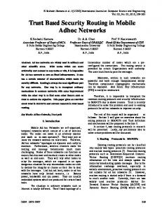
3. PARALLELIZATION AND REPLICATION We have extended our prototype compiler to perform different parallelization and replication strategies to optimize the execution of iterations of a spatial view iterator. The initial implementation as discussed in [21] uses a single instance of the program that migrates from one virtual node to another. Through replication, multiple serial program executions can be initiated on the injection node. Each of these clones is independent. The final answer of the execution of the iterator is determined by the first clone that returns to the injection node. A parallel strategy constructs a spanning tree to reach all virtual nodes. Once an iteration has been performed, all virtual nodes reachable from the current virtual node receive a copy of the program. This is basically a fork operation. The parent will wait until all children have reported back, and then will process and pass on its results to its parent, and so on. An implicit timeout operation ensures that a parent does not wait indefinitely for a child since a child may have died due to node failure. In this scheme, all nodes along the spanning tree cooperate to produce the final result. The flooding version of this scheme constructs the spanning tree each time the program is injected. In contrast, the tree-based version reuses the spanning tree from previous executions by storing the routing tables in each visited node. These different approaches are illustrated in Figure 2. The figure does not show the replicated serial case. The compiler allows the selection of any of these approaches through a command line option. The pseudocode describing a framework for the parallel approaches, i.e. the cooperative and the tree-based approaches, is given in Figure 3. There are three hook functions in the framework, namely usertask(), merge(), and readback(). These hook functions are generated by the compiler. Most of the iteration body is put in usertask(), which defines the computation to be executed on an interesting node. Partial results are merged in merge() using reduction operations applied to reduction variables. readback() puts the updated values of reduction variables in the data brick of the Smart Message, so that they will be communicated back to the parent node. The cooperative and the tree-based approaches shared the framework but differ in how they discover neighbors. The flooding approach discovers neighbors in the original network, while the tree-based approach discovers neighbors through the recorded spanning tree. As mentioned in Section 2.2 SpatialViews supports reduction variables, for instance sum reductions with operators “++” and “+=”. The current compiler performs reduction variable recognition and makes sure that reduction variables are not read or written anywhere in the iteration other than through reduction operations. Reduction variables are put into the data brick of the generated Smart Message program. They are partially calculated in usertask(), updated in merge(), and then put back into the data brick in readback(). Local variables that are read-only are also put in the data brick, but their values are not updated when migrating back. The current implementation does not support parallelization of iterations with container variables.
(a) Serial (independent)
(b) Flooding (cooperative)
(c) Tree-Based (cooperative)
Figure 2: Three Possible Approaches for Spatial View Iterations For each reduction variable, the SpatialViews program creates a tag on the node. The tag space is a non-migratory memory space on each node, which also provides a synchronization mechanism to Smart Messages[17]. After local computation is done, the program writes the partial result for each reduction variable to its tag. Once the child threads returns with its partial results, the results are merged into the corresponding tags. In the end, the parent program reads the tag, puts its content into the data bricks, and migrates one-hop back toward the starting node. Figure 4 shows parts of the generated code for the lighting example. This code combined with the framework in Figure 3 provides a parallel implementation of the SpatialViews program shown in Figure 1. Our current prototype compiler produces as output bytecode. The Smart Messages system [17] is an extension of the Java 2 Platform, Micro Edition (J2ME)[13]. The Kilobyte Virtual Machine (KVM)[14] and the Connected, Limited Device Configuration (CLDC) class libraries were modified to implement light-weight process migration. J2ME has been widely used in today’s cell phones. It has a footprint of only 128KB. Some other Java implementations even even smaller footprints. For example, Waba[3] requires less than 64KB RAM and JBlend[1] can run in less than 30KB RAM. Figure 5 shows the structure of our SpatialViews prototype compiler. We modified the Java compiler (javac in the suite J2SDK 1.3.1) from SUN Microsystems. The parser was changed and the intermediate representation (IR) was enriched. An IR translator was built to parallelize spatial view iterations. Standard Java bytecode is generated from the translated IR. Like any other J2ME program, the generated bytecode has to be preverified before it can run on the Kilobyte Virtual Machine (KVM). Figure 6 shows the run-time environment for the final pre-verified bytecode.
iterate() { if (this node has been visited or some limit has been exceeded) return; Mark the current node as visited. usertask(); // Hook function for the computing task. spawn(); // Copy myself if (this is the parent thread) Block until all children report back or time out. else { // This is the child thread prev_node = current node address; Discover all neighbor nodes; Propagate to neighbors; iterate(); migrate(prev_node); // Migrate one-hop back. merge(); // Hook function to merge partial results Inform the parent process that I am back exit(0); // Child thread kills itself. } readback(); // Hook function to pack partial results } Figure 3: Parallel Iteration Framework
// s and n are defined in the data brick and // are carried in a migration float s; int n; userTask() { writeTag(‘‘s’’, x.read()); writeTag(‘‘n’’, 1); } merge() { try { s += readTagAsFloat(‘‘s’’); n += readTagAsInt(‘‘n’’); } catch (TagNotFoundException e) { // No previous partial result is found } writeTag(‘‘s’’, s); writeTag(‘‘n’’, n); } readback() { s = readTagAsFloat(‘‘s’’); n = readTagAsInt(‘‘n’’); }
Figure 5: Compilation Flow for a Spatial Views Program Spatial Views Applications Spatial Views Library Smart Message Virtual Machine
Figure 4: Code Generated for the Lighting Example Tag Space & Code Cache
4.
EXPERIMENTAL EVALUATION
A series of experiments were performed to evaluate the different compilation approaches with respect to three metrics, namely response time, quality of result, and energy consumption under varying node failure rates. Some results were obtained using a validated analytical model of failure resilience, some using simulations, and others were based on physical measurements. The benchmark programs for the experiments were mostly different versions of the LightSensor application shown in Figure 1. In our testbed, the mobile network nodes were HP/Compaq iPAQ pocket PC’s (H3600, H3700, and H3800 series) with wireless 802.11b connections in ad-hoc mode. We used up to 16 iPAQs in the experiments. MIT’s Crickets indoor location system was used to provide location information [2, 23, 22]. All iPAQs ran Familiar Linux v0.6.1 or v0.7.2 and J2ME with the SpatialViews runtime environment and Smart Messages extension. Different sets of experiments were performed for each performance metric. The results are reported in the next sections.
4.1 Response Time The first experiment ran the average lighting application shown in Figure 1. Six iPAQ handheld PCs were used in this experiment with a fully-connected network topology, i.e. any pair of iPAQs was connected in the network. The network topology was kept stable across successive program executions, resulting in the same network topology to be discovered by the program. Figure 7 shows the execution times for 21 successive executions. The initial drop in execution time for the tree-based approach can be partly attributed to code caching done by the Smart Messages runtime system. The tree-based approach is much faster than the flooding approach in the long-term, because 1) it does not migrate
Figure 6: Runtime Environment beyond leaf nodes (while the flooding approach has to go further to find out if other nodes are visited or not), and 2) it does not query the location service on each node since the spanning tree has already been built, so the interesting nodes on the tree have been verified locating in the interested space. A positioning operation based on MIT Crickets can take as long as 4 seconds. The second experiment used a network with a binary tree topology. The size of the network varied from 2 to 16 nodes. For this experiment we used a counting example program similar in structure to the lighting example, but without method calls to read a sensor. The target spatial view was the whole network and no query to the location service was issued. We ignored the initial program execution to avoid the effect of Smart Message code caching. The results for the flooding and the tree-based approaches were identical since the underlying topology was already a tree. Figure 8 shows the average execution times for different network sizes. Again, the network was kept stable.The experiment showed that parallel execution (the cooperative or the tree based approach) scales significantly better than the serial execution using a single program copy. The parallel version was twice as fast as the serial version with 8 nodes, and about 3 times faster with 16 nodes. We did not consider replication of the serial case here since the execution times will be larger due to node and network contention.
4.2 Failure Resilience
30.6*x**60.2 10
1
0.1
0.01 0.9
0.92
0.94
0.96
0.98
1
Avg. number of nodes visited
Avg. number of nodes visited
100
32.5 31*x+1 32 31.5 31 30.5 30 29.5 29 28.5 0.9
Node Availability
20 15 10 5 0 0.92
0.94
0.96
0.98
1
Node Availability (c) Redundant
Avg. number of nodes visited
Avg. number of nodes visited
3 instances 5 instances 7 instances
0.9
0.96
0.98
1
(b) Cooperative
35
25
0.94
Node Availability
(a) Serial
30
0.92
35 30 Cooperative Serial 8 instances 32 instances 128 instances 512 instances
25 20 15 10 5 0 0.9
0.92
0.94
0.96
0.98
1
Node Availability (d) Theoretical
Figure 9: Failure Resilience of Different Compilation Approaches Failure is not an uncommon event in our ad-hoc mobile target network. In this section we investigate the impact of node failure on the quality of the program answer. We assume that the quality of the answer directly correlates to the number of visited nodes that manage to report back to the program injection node. Only node failures were used to evaluate the failure resilience of the different parallelization and replication approaches. Failures such as network link failures were not considered. Our experiments used a migration-driven node failure model. Every time a program migrates to a node, we consider the program’s successful execution on that node as a trial. If the node fails during the program’s execution, the trial fails, and otherwise it succeeds. Let a denote the probability that the trial succeeds, then p = 1 − a is the probability that it fails. For the following discussion, we call p the node failure probability and a the node availability. As a simple interpretation of this failure model, imagine we toss a coin every time the
program migrates to a node. If the outcome is head (with a probability of p), the program gets killed. Otherwise, the program executes to completion on the node and then migrates to another node. There are more realistic and more complicated failure models such as time-driven models. Let X denote the time until a node failure occurs. X is a random variable with exponential distribution. In a time-driven model, we simulate X for each node and bring down the node at time X. All the programs running on a node at the time it is killed are aborted. A time-driven model is more realistic in that it considers the amount time that a program spends on a node, which potentially affects how likely the program will get killed by a node failure. However, simulating a time-driven model requires a stand-alone deamon running on each node which generates failures. In the migration-driven model, we can simply implant code into the tested program itself that “tosses a coin” after each migration to determine the program’s fate.
The average number of visited nodes is na2n−3 . Figure 9(a) shows the experimental results, which well fit the formula. The axes are both in log scale.
Execution time (ms)
30000 tree-based cooperative serial
25000 20000 15000 10000 5000 0 0
5
10
15
20
Time Figure 7: Response Times for All Three Approaches for 21 Successive Exections in a Stable Network
Execution time (ms)
1800 parallel serial
1600 1400 1200 1000 800 600 400 200 0 0
2
4
6
8
10
12
14
16
Number of Nodes
Figure 8: Scalability Comparison: Parallel v.s. Serial We simulated node failures on all the nodes except the node where the program starts and returns. We ran the light sensor program multiple times for a given node failure probability and calculated the average number of visited nodes across the multiple runs as a metric for quality of results. For highly unreliable nodes, we ran the program as many as 2,000 times. With the serial, cooperative, and redundant approaches, we repeated the experiment for different node availabilites. We did the experiments by running 32 Java virtual machines on a single PC. The virtual machines were the same as those running on our iPAQ network nodes. This way, we could study a network of a larger size than our physical equipments allowed. The 32 “nodes” of this experiment were fully connected. For the serial approach, if there is a node failure, the program dies and never reports back. The observed quality of result is thus 0. If no node fails, the quality of result is the number of all the nodes in the network. The probability for the program to return successfully is a2n−3 , where n is the number of nodes in the network, n = 32 for our experiments.
For the cooperative flooding approach, if there is a node failure, only the partial results from that node will be lost. This implies the number of visited nodes is a binomial random variable. Assuming the starting node never fails, the quality of result for the cooperative approach is (n − 1)a + 1 in a fully-connected topology. This was verified by the experimental results shown in Figure 9(b). If the network connectivity goes down, the quality of result for flooding will degrade. In the worst case, when the network is a chain, flooding has the same quality of result characteristic as the serial version. In the replication approach, we get all the nodes if any instance comes back, but 0 if none of them comes back. The 2n−3 probability for the latter is pm and m 1 , where p1 = 1 − a is the number of redundant program instances (clones). The 2n−3 m quality of result is therefore n(1−pm ) ), 1 ) = n(1−(1−a where m is the number of instances we have for the same program. Figure 9(c) shows the experimental results for 3, 5, and 7 serial clones, together with the theoretical analytically obtained results for the same replication factors. The experimental results fit the analytical formula above. Figure 9(d) shows the theoretical curves for serial, flooding, and replicated approaches. The number of redundant instances are m = 8, 32, 128, and512. The numbers show that overall the serial approach has the worst resilience to failures and the flooding approach has the best. However, serial replication shows clear improvements over the simple serial approach, but needs a significant degree of replication to get close or outperform the flooding approach. This is because the success rate for a serial execution is so low that simply repeating it a few times does not increase the overall success rate very much.
4.3 Energy Consumption The experimental results reported in the previous sections seem to favor parallel execution. However, parallel execution may result in heavier network traffic and contention, and more computation, which in turn may lead to higher power and energy consumption. Power Supply Oscilloscope
Current Samples iPAQ
Data Via Ethernet
Data Acquisition Computer
iPAQ
... iPAQ
Figure 10: Energy Measurement Setup
We connected 8 iPAQ’s with BackPAQ camera sleeves to a single DC power supply in parallel. An oscilloscope was used to measure the current at the output of the power supply. The current readings were collected by a data acquisition PC. Figure 10 shows a diagram of the testbed setup. We calculated the power dissipation of all the iPAQ’s from the current readings and the input voltage of 5V. Due to the fact that all batteries were fully charged before the experiments and the iPAQ’s DC/DC converters are highly efficient, the observed power dissipation should be very close to the actual power dissipation of the network. To evaluate the energy consumption of different compilation approaches, we did experiments on the 8 iPAQs and a laptop. We ran a modified lighting sensor program where the computation load for each iteration was increased to take approximiately 1 second. The replication factor (redundancy) varied from 2 to 9. The program starts on the laptop and visits all the iPAQs if no failure occurs. Figure 12 shows the current change. The oscilloscope sampling frequency was every 4 millisecond. There were 10,000 samples for each experiment. Figure 12 also shows the execution time for the program with vertical lines. In the case of redundant iterations, it shows the times for all the instances. Due to measurement error, the real execution time was about 0.5 to 1 second longer than seen in the figures. With each curve in Figure 12, we could calculate the energy consumed by the iPAQ network during the 40 seconds (the program started at second 0). The energy, denoted as Etotal , is the integration of that curve, multiplied by the voltage (5 volts.) We could also calculate the energy if the network remained idle for 40 seconds, denoted as Eidle , integrating the idle state region only and extrapolating the result to a 40second period. The extra energy consumption caused by the execution of our program was E = Etotal − Eidle . Figure 11 shows the energy consumption(E) using different compilation approaches and different node availability rates. It is important to note that the listed numbers are average numbers over several program exectutions. In terms of quality of result, a single replicated program can either terminate successfully with the perfect answer resulting from 9 node visit, or not produce any answer at all. The fact that we report fractions in the range of 0 and 9 is due to the distribution of successful vs. failed program executions. We have the following observations about Figure 11(a). 1. The cooperative approach has similar energy consumption as the serial approach (in fact slightly better in our experiment.) This can be explained by the fact that the cooperative approach does not increase the total work done by the system as compared to serial approach, although it reduces the time to finish the work. Because it does the same work in shorter time, the cooperative results in higher power dissipation (work per unit time) as seen in Figure 12. However, we have to keep in mind, by doing the total work faster, we may increase the communication contention because the communication media (the radio spectrum) is shared and accessed by all the nodes. This is especially true if we have communication dominant programs, which is not the case in our experiments due to the workload of approx. 1 second per
iteration. 2. In the case of replicated serial execution, an increase in the degree of replication is directly reflected in the resulting increase in energy consumption. This can be explained by the fact that doubling the work should result in at least doubling the energy consumption. 3. The flooding and tree-based approaches are much more energy efficient than the replication approaches. This is a conclusion of Observation 1 and Observation 2. The maximum activity for the flooding approach is one program instance per node, i.e., 9 program instances in the network for our experiment. However, the flooding approach for node availabilty of 99% is much more energy-efficient (12.69 joules v.s. 116.68 joules) than the redundant approach with the same maximum activity, i.e., the 9-instance redundant approach. Even if we consider the average activity and be conservative, and assume the average activity for the cooperative approach is only equivalent to the 2-instance redundant approach, we still see its advantage (12.69 joules v.s. 23.70 joules.) A possible justification is as follows: In the redundant approach, the program instances do not cooperate with each other, while in the cooperative approach, the program instances share the partial results and avoid visiting the same nodes. Non-cooperation is inefficient since it not only increases the activity to get the real work done, but it also increases contention for communication and computation resources. Similar results hold for node availability of 90%. 4. The tree-based approach consumes more energy than the flooding approach in the initial run. The extra energy consumption is attributed to building the spanning tree. 5. The tree-based approach consumes less energy than the flooding approach after the initial run. This is because it saves the work for discovering interesting nodes. 6. The tree-based approach after the initial run is the most energy efficient among all the approaches. This is the conclusion of all the above observations. However, this is not always true and has to be understood in the context that the network has to remain rather stable over time for the tree-based approach to be beneficial. In contrast, Observation 3 is always true. 7. The average response time for the replication strategies decreases from the 99% availability to the 90% case, while they increases for the cooperative cases. The reason is that fewer replication survive, resulting in less contention. The increase for the cooperative case is due to the waiting times for aborted children. The parent has to wait until a predefined timeout has expired before it can proceed.
We predicted the average number of visited nodes using the model verified in Section 4.2. The prediction is shown in all four subfigures of Figure 11 in shaded bars. The single node availability is assumed to be 99% and 90%. As can be easily seen by comparing Figures 11(a) and Figures 11(c), the
(a) Energy consumption (a=99%)
(b) Response time (a=99%)
(c) Energy consumption (a=90%)
(d) Response time (a=90%)
Figure 11: Energy and Response Time (solid bars) v.s. Failure Resilience (shaded bars) failure resilience characteristics depend on the overall node availability. We should emphasize that the system failure resilience depends on the network size as well. A comparison between Figures 11(a) and 11(c) for energy consumption and Figures 11(b) and 11(d) show different tradeoffs between energy consumption, performance and average quality of result for node availabilities of 90% and 99%. For instance, if an execution based on replication requires an average quality of result of at least seven visited nodes, the serial version is sufficient for the 99% case, but the 90% case needs at least seven instances. If a perfect result is required, i.e., if a perfect answer is expected nearly all of the time, a replication of degree three or four is appropriate for the 99% case, but not possible with less than nine instances for the 90% node availability. Similar tradeoffs can be observed for response time.
Finally, Figure 12 can be used to derive the peak power dissipation of the different program optimizations. Peak power can be used as an indicator of program activity. Without loss of generality, we will discuss only the serial, the cooperative, and the 9-instance redundant approaches. For Figure 12(a), 12(i), and 12(j), we picked a peak region and a idle region for each of them, and calculated the power in those regions. The results are following. In Table 4.3, the 9-instance redundant approach has a 5.4 times power increase as compared to the serial approach, while a 9 fold increase could be expected. The reason is that the 9 instances started on the same node, and at one time only one instance got the chance to execute. After the instances slowly fanned out to multiple nodes, they still competed for the communication media. The contention continues since different copies may encounter each other on some node and compete for the computation resource. The coop-
Compilation approach Serial 9-instance Redundant Flooding
Ipeak [5s,10s] [12s,16s] [6s,40s]
Ppeak 25.61 28.88 29.51
Iidle [20s,35s] [39.6s,40s] [1s,2.5s]
Pidle 24.89 24.96 24.8
∆Ppeak 0.72 3.92 4.68
Table 1: Peak power increase with different compilation approaches. (Ipeak is the peak region, Ppeak is the peak power in watts, Iidle is the idle region, Pidle is the idle power in watts, and ∆Ppeak is the peak power increase in watts.) erative approach is better, with a 6.5 times increase. But 8 fold increase was expected, since there could be 8 nodes running simultaneously. However, due to communication contention, a lower increase was seen.
5.
RELATED WORK
Programmability of ad-hoc networks has become a research focus [26, 25, 9, 12, 19, 20, 6]. Hood[26] and Abstract Regions[25] provide similar abstractions as SpatialViews , i.e., grouping nodes based on their properties. Hood is a low-level data sharing mechanism among neighboring nodes which could serve as a target language for SpatialViews on sensor networks. Abstract Regions provides a similar group data sharing abstraction and collective operations with fidelity feedbacks and tuning options. TinyOS[12] and nesC[9] provide a component-based event-driven programming environment for Berkeley Motes. nesC is an extension to C that supports and reflects TinyOS’s design. TinyOS and nesC use Active Messages as a communication paradigm. Active Messages has a similar flavor to execution migration of SpatialViews , but use non-migrating handlers instead of migrating code. Mat´e[19] is a tiny virtual machine built over TinyOS for sensor networks. It allows capsules in bytecode to forward themselves through a network with a single instruction, which bears the resemblance to execution migration in SpatialViews . Self forwarding enables online software upgrading, which is important in large-scale sensor networks. Impala[20] also provides an event-based programming model, and emphasizes issues such as on-line software updates and adaptability. SensorWare [6] provides lightweight mobile scripts for sensor networks and is very similar to Smart Messages. The SpatialViews service discovery feature is similar to systems like Jini[24] or INS[4], but in contrast to these system it is not based on complex static directories. Migratory execution as seen in SpatialViews and implemented by Smart Messages has been extensively studied in the literature, especially in the context of mobile agents[11, 10]. However, SpatialViews only supports implicit transparent migration hidden in its iteration operation, and names a node using a service and a space. This is novel compared to previous mobile agent systems. SpatialViews deals with resource constraints, e.g., time constraint as we first proposed in [21]. However the time constraint in SpatialViews is significantly different from previous systems with strict time constraints, e.g. the time constraints in the Time Warp OS[15]. In Time Warp OS, the messages generated by a parallel discrete event simulation system have to be received in a nondecreasing timestamp order. This restriction can never be violated in order to guar-
antee the correctness of the simulation. Time Warp OS uses a process rollback mechanism to implement the time constraints. In contrast, the time constraint in SpatialViews is a soft deadline which should be better described as a budget. It is the amount of time that a programmer is willing to spend to finish a spatial view iteration. If the program spends more than the budget, further iteration will be prevented, but no rollback is necessary if ever possible. The time constraint in SpatialViews is one way for the programmer to tune the trade-off between the iteration time and the quality of results. Solar[8] proposed an infrastructure with a programming model implemented in a set of Java API’s for context-aware mobile applications. It is an event-driven model. Context information, e.g. location from an IR-based location system, is abstracted as events, generated by sources. Events are handled by operators which form a network and eventually route events to subscribing applications. A programmer is allowed to derive new sources and operators from the API’s.
6. CONCLUSION AND FUTURE WORK
SpatialViews is a programming language for dynamic networks of mobile devices and embedded systems. In such environments, the physical locations of nodes are crucial. SpatialViews allows a programmer to specify a virtual network based on common node characteristics and location. Nodes in such a virtual network can be visited using an iterator. Execution migration, node discovery, and routing are transparently supported. Energy efficiency and failure resilience is also important in a network of mobile devices. In this paper, we presented experimental and analytical results that indicate the tradeoffs between different optimizations of spatial view iterations. Based on a SpatialViews prototype compiler, the performance metrics of different parallelization and replication strategies were evaluated. These performance metrics are overall program response time, energy consumption, and quality of the produced answer. As one of the the first location-aware programming languages for ad-hoc networks of mobile devices, SpatialViews is simple and expressive. A SpatialViews prototype compiler and runtime library have been implemented as an extension to J2ME. Experimental results on a network of up to 16 iPAQ handheld computers showed that the compiler is effective in parallelizing SpatialViews programs. The SpatialViews language and compiler are still under development. As one direction of our future work, optimizations like parallelization combined with location information will be explored. The tuning of cooperative approaches in a failure
7
7
6.5
6.5
5.5 5 4.5
6
Current(A)
6
Current(A)
Current(A)
7 6.5
5.5 5 4.5
4
4
4
3.5
3.5
3 0
5
10 15 20 25 30 Time(seconds)
35
40
3 0
5
10 15 20 25 30 Time(seconds)
35
40
0
(b) 2 instances
7
7
7
6.5
6.5
5 4.5
6
Current(A)
6 5.5
5.5 5 4.5
4 3.5
3 35
40
5
10 15 20 25 30 Time(seconds)
35
40
0
(e) 5 instances
7
7
7
6.5
6.5
6
Current(A)
Current(A)
5 4.5
5.5 5 4.5 4
4 3.5
3 10 15 20 25 30 Time(seconds)
35
40
5
10 15 20 25 30 Time(seconds)
35
40
0
7
7
7
6.5
6.5
6
Current(A)
Current(A)
5 4.5
5.5 5 4.5
5 4.5
4
4
4
3.5
3.5
3 5
10 15 20 25 30 Time(seconds)
(j) Cooperative
35
40
40
6 5.5
3.5 3
10 15 20 25 30 Time(seconds)
(i) 9 instances
6.5
0
5
(h) 8 instances
6
35
3 0
(g) 7 instances
5.5
40
5 4.5
3.5 5
35
6
4
0
10 15 20 25 30 Time(seconds)
5.5
3.5 3
5
(f) 6 instances
6.5 6
40
3 0
(d) 4 instances
5.5
35
5
4
10 15 20 25 30 Time(seconds)
40
4.5
3.5 5
35
6
4
0
10 15 20 25 30 Time(seconds)
5.5
3.5 3
5
(c) 3 instances
6.5 Current(A)
Current(A)
(a) Serial
Current(A)
5 4.5
3.5 3
Current(A)
6 5.5
3 0
5
10 15 20 25 30 Time(seconds)
35
(k) Tree-Based(Initial Run)
40
0
5
10 15 20 25 30 Time(seconds)
(l) Tree-Based(After Initial Run)
Figure 12: Current of 8 iPAQ’s Running with Different Approaches
prone network is another area of future work.
7.
REFERENCES
[1] Applix’s jblend. http://www.aplixcorp.com/products/jblend.html. [2] The cricket indoor location system. http://nms.lcs.mit.edu/projects/cricket. [3] Waba programming platform. http://www.wabasoft.com. [4] W. Adjie-Winoto, E. Schwartz, H. Balakrishnan, and J. Lilley. The design and implementation of an intentional naming system. In SOSP, 1999. [5] C. Borcea, C. Intanagonwiwat, P. Kang, U. Kremer, and L. Iftode. Spatial programming using Smart Messages: Design and implementation. In International Conference on Distributed Computing Systems (ICDCS’04), Tokyo, Japan, March 2004. [6] A. Boulis, C. Han, and Mani Srivastava. Design and implementation of a framework for efficient and programmable sensor networks. In MobiSys, 2003. [7] N. Carriero and D. Gelernter. Linda in context. Communications of the ACM, 32(4):444–458, April 1989. [8] Guanling Chen and David Kotz. Solar: A pervasive-computing infrastructure for context-aware mobile applications. Technical Report TR2002-421, Department of Computer Science, Dartmouth College, February 2002. [9] David Gay, Phil Levis, Robert von Behren, Matt Welsh, Eric Brewer, and David Culler. The nesC language: A holistic approach to networked embedded systems. In PLDI, 2003. [10] Robert S. Gray. Agent Tcl: A flexible and secure mobile-agent system. PhD thesis, Dartmouth College, June 1997. [11] Robert S. Gray, George Cybenko, David Kotz, Ronald A. Peterson, and Daniela Rus. D’agents: Applications and performance of a mobile-agent system. Software: Practice and Experience, May 2002. [12] Jason Hill, Robert Szewczyk, Alec Woo, Seth Hollar, David Culler, and Kristofer Pister. System architecture directions for network sensors. In ASPLOS, 2000. [13] Sun Microsystems Inc. Java 2 Platform, Micro Edition (J2ME). [14] Sun Microsystems Inc. KVM White Paper. [15] David Jefferson, Brian Beckman, Fred Wieland, Leo Blume, Mike DiLoreto, Phil Hontalas, Pierre Laroche, Kathy Sturdevant, Jack Tupman, Van Warren, John Wedel, Herb Younger, and Steve Bellenot. Distributed simulation and time warp operating systems. In SOSP, 1987.
[16] P. Juang, H. Oki, Y. Wang, M. Martonosi, L-S. Peh, and D. Rubensteing. Energy-efficient computing for wildlife tracking: Design tradeoffs and early experiences with zebranet. In Thenth International Conference on Architectural Support for Programming Languages and Operating Systems (ASPLOS-X), San Jose, CA, October 2002. [17] Porlin Kang, Cristian Borcea, Gang Xu, Akhilesh Saxena, Ulrich Kremer, and Liviu Iftode. Smart messages: A distributed computing platform for networks of embedded systems. The Computer Journal, Special Issue on Mobile and Pervasive Computing, 47(4), January 2004. [18] U. Kremer, J. Hicks, and J. Rehg. A compilation framework for power and energy management on mobile computers. In International Workshop on Languages and Compilers for Parallel Computing (LCPC’01), Cumberland, KT, August 2001. [19] Philip Levis and David Culler. Mate: A tiny virtual machine for sensor networks. In ASPLOS, 2002. [20] Ting Liu and Margaret Martonosi. Impala: a middleware system for managing autononmic parallel sensor systems. In PPoPP, 2003. [21] Yang Ni, Ulrich Kremer, and Liviu Iftode. Spatial Views: Space-aware programming for networks of embedded systems. In The 16th International Workshop on Languages and Compilers for Parallel Computing (LCPC 2003), October 2003. [22] Nissanka B. Priyantha, Anit Chakraborty, and Hari Balakrishnan. The cricket location-support system. In MobiCom, 2000. [23] Nissanka B. Priyantha, Allen K. L. Miu, Hari Balakrishnan, and Seth J. Teller. The cricket compass for context-aware mobile applications. In MobiCom, 2001. [24] Jim Waldo. The Jini architecture for network-centric computing. ACM Communications, July 1999. [25] Matt Welsh and Geoff Mainland. Programming sensor networks using abstract regions. In NSDI 2004, March 2004. [26] Kamin Whitehouse, Cory Sharp, Eric Brewer, and David Culler. Hood: A neighborhood abstraction for sensor networks. In Mobisys 2004, June 2004.