Electronic Notes in Theoretical Computer Science 84 (2003) URL: http://www.elsevier.nl/locate/entcs/volume84.html 12 pages
A Programming Language for the Interval Geometric Machine Renata Hax Sander Reiser 1 Antˆonio Carlos da Rocha Costa 2,4 Gra¸caliz Pereira Dimuro 3 Escola de Inform´ atica Universidade Cat´ olica de Pelotas Pelotas, 96010-000, Brazil
Abstract This paper presents an interval version of the Geometric Machine Model (GMM) and the programming language induced by its structure. The GMM is an abstract machine model, based on Girard’s coherence space, capable of modelling sequential, alternative, parallel (synchronous) and non-deterministic computations on a (possibly infinite) shared memory. The processes of the GMM are inductively constructed in a Coherence Space of Processes. The memory of the GMM, supporting a coherence space of states, is conceived as the set of points of a three dimensional euclidian space. The version of the GMM presented here operates with real intervals, and is defined to model the semantics of algorithms of Interval Mathematics. Using the programming language induced by such structure, simple interval algorithms are presented, and their domain-theoretic semantics in the machine model is given.
1
Introduction
In this work, aspects of Domain Theory [1] and Concurrency Theory [4] are connected in order to obtain a semantics for interval algorithms [5] involving non-deterministic and synchronous parallel computations performed over matrix structures, based on Girard’s Coherence Spaces [3]. The work presents an interval version of the Geometric Machine Model (GMM) where the possibly infinite set of memory positions are labelled by points of the three-dimensional euclidian geometric space. This model is able to describe partial computations and to formalize non-determinism and concurrency in the accesses to memory 1 2 3 4
Email:
[email protected] Email:
[email protected] Email:
[email protected] PPGC, Universidade Federal do Rio Grande do Sul, Porto Alegre, Brazil
c 2003 Published by Elsevier Science B. V. °
Reiser, Costa and Dimuro
positions. To define this model, the following ordered structures are considered: the domain of states S, the domain of boolean tests B and the domain of processes D→ ∞ . Also, the coherence space IIQ of rational intervals [2] is taken into account, to model the data operated by the processes. The input and of output data S of the GMM are defined on the the extended set of real intervals IR = IR {(−∞, +∞)}. The interval version of the GMM is called Interval Geometric Machine (IGM). This paper is organized as follows. In Section 2 basic concepts of coherence spaces and linear functions are considered together with the ordered structure of the IGM model. Section 3 introduces the language L(D→ ∞ ) derived from D→ . The formal definition of the IGM model is presented in Section 5 and ∞ the last section shows some intervals algorithms expressed in L(D→ ∞ ).
2
The Ordered Structure of the IGM Model
2.1
Coherence Spaces and Linear Functions
A web W = (W, ≈W ) is a pair consisting of a set W with a symmetric and reflexive relation ≈W , called coherence relation. A subset of this web with pairwise coherent elements is called a coherent subset. The collection of coherent subsets of the web W, ordered by the inclusion relation, is called a coherence space, denoted by W ≡ (Coh(W), ⊆) [10]. Linear functions are continuous functions in the sense of Scott [1] also satisfying the stability and linearity properties that assure the existence of least approximations in the image set [10]. Considering the coherence spaces A and B, a linear function f : A → B is identified by its linear trace, a subset of A × B given by ltr(f ) = {(α, β) | β ∈ f (α)}. Let A ( B = (A × B, ≈ ( ) be the web of linear traces with the coherence relation given by (α, β) ≈( (α0 , β 0 ) ↔ ((α ≈A α0 → β ≈B β 0 ) and (β = β 0 → α = α0 )). The collection of coherent subsets of the web A ( B, ordered by inclusion relation, defines the domain A ( B ≡ (Coh(A ( B), ⊆) of the linear traces of functions from A to B. In the following, we summarize the construction of the ordered structure of the IGM model, based on coherence spaces and traces of linear functions. For more details, see [6]. 2.2
The Coherence Space of Machine States
The notion of memory state in the IGM model is formalized as follows. Consider the flat domain R3 ≡ (Coh(R3 , =), ⊆) of memory positions, representing names of variables. Let IIQ ≡ (Coh(IQ), ⊆) be the Bi-structured Coherence Space of Rational Intervals [2], representing the values that can be assigned to the variables. This domain is defined on the web IQ = (IQ, ≈IQ ), given by the set of rational intervals with the coherence relation p ≈IQ q ↔ p ∩ q 6= ∅. This representation of the computable real numbers and the real intervals was 2
Reiser, Costa and Dimuro
introduced in [2]. As suggested in [8], deterministic machine states are modelled as functions from memory positions to values. Non-deterministic machine states are modelled as families of deterministic machine states (with singletons modelling deterministic states). Definition 2.1 Let R3 ( IIQ be the coherence space modelling deterministic machine states, and S = (Coh(R3 ( IIQ), ≈S ) be the web given by the set of all coherent subsets of R3 ( IIQ, together with the trivial (i.e., universal) coherence relation ≈S . The collection of all coherent subsets of S, ordered by inclusion, defines the coherence space that models the non-deterministic (and the singleton deterministic) machine states, denoted by S ≡ (Coh(S), ⊆). A machine state is conceived then as a coherent set of linear traces of strict, continuous, stable and linear functions from R3 to IIQ, one trace for each deterministic component of the non-deterministic state. 2.3
The Set D0 of Elementary Processes
The intuitive notion of an elementary process, which modifies a single memory position in a single unit of computational time (uct), can be described by an elementary transition between deterministic memory states, given by a linear function. Its intuitive representation in a one-dimensional machine is in Fig. 1(a). It is a function d(k) satisfying: Proposition 2.2 Let A ≡ [R3 ( IIQ] ( IIQ be the coherence space of the so-called computational actions. If d, pr(k) ∈ A, with pr(k) (s) = s(k) then the function d(k) ∈ [R3 → IIQ] → [R3 → IIQ] given by pr(i) (s) = s(i) if i 6= k, d(k) (s)(i) = d(s) if i = k
is a linear function.
Proof. Let s0 , z 0 ∈ [R → IIQ], i, k ∈ IIQ and s0 = d(k) (s), z 0 = d(k) (z). We show that, for all (s, s0 ), (z, z 0 ) in the graph of the function d(k) the following properties hold. (1) If s ≈( z then s0 ≈( z 0 : Suppose s ≈( z. If i 6= k and d ∈ [R ( IIQ] ( IIQ then d(k) (s)(i) = s(i) ≈IQ z(i) = d(k) (z)(i). In the other case, if i = k then d(k) (s)(k) = d(s) ≈( d(z) = d(k) (z)(k). Thus, s0 ≈( z 0 . (2) If s0 = z 0 then s = z: Suppose s0 = z 0 . When i 6= k and d ∈ A is a linear function, s(i) = d(k) (s)(i) = s0 (i) = z 0 (i) = d(k) (z)(i) = z(i) then s = z. Otherwise, if i = k, d(k) (s)(i) = d(s)(k) = d(z)(k) = d(k) (z)(i) and s = z based on the linearity of function d. Thus, in any case, s = z, and d(k) is linear. 2 Fig. 1(b) schematically represents the elementary processes in d(k) . The identity function interprets the undefined process skip (Fig. 1(c)). 3
Reiser, Costa and Dimuro
s d (n) s'
v0
v1
...
vn
...
pr
pr (1)
...
d
...
v0
v1
...
d(s)
...
dn
(b)
skip
(c)
t
(a)
ek
dk
(e)
el
dk
(f)
(d)
dk (h)
t
dk
el
(g)
el
Fig. 1. Diagrammatic representation of one-dimensional computational elements.
2.4
The Coherence Space of Boolean Tests
To represent the deterministic sums of processes, we consider the set B of boolean tests related to the binary logic and assume the Coherence Space B of Boolean Tests as the set of all coherent subsets of tests of the discrete web B ≡ (B, =), ordered by the inclusion relation. The coherence space S ( B models the boolean tests t (see Figure 1(d)). Non-determinism enforces a non-traditional treatment of tests. For each boolean test b capable of testing a deterministic state s, we consider two forms for tests b on non-deterministic states s: (i) a universal form (b ∀ (s) ≡ ∀s ∈ s . b(s)) and (ii) an existential form (b∃ (s) ≡ ∃s ∈ s . b(s)). Both forms coincide with the simple test b when s is a deterministic singleton set. 2.5
The Coherence Space of Processes D→ ∞
In this section, we summarize the main properties of the Coherence Space D→ ∞ of processes in the IGM model, inductively constructed 5 from the coherence space D0 of elementary processes. Following the methodology proposed in [9], each level in the inductive construction is identified by a subspace Dn , which reconstructs all the objects from the level below it, preserving their properties and relations, and constructs the new objects specific of this level, see Fig. 2. The constructive relationship between the levels is expressed by linear functions called embedding and projection functions, interpreting constructors and destructors of processes, respectively. In the next subsection, we summarized important aspects of each level of such inductive construction. 2.5.1 The basic level of the inductive construction of D→ ∞ Let D0 ≡ (D0 , =) be a discrete web defined by the set D0 of elementary processes ( 2.3) with the equality relation. D0 = (Coh(D0 ), ⊆) denotes the 5
The Coherence Spaces constructors used in the definition of D→ ∞ can be found in [10].
4
Reiser, Costa and Dimuro
Dω
2 ω uct
Dω
... 2 n+1 uct
D n+1
1
Pn P n temporal interpretations
1 π n ,Π n
D n+1
2 uct
... 2 1 uct
Dn
Pn 0
Dn
D1
D1
D0
D0
π 0 ,Π 0
2 0 uct
concurrent processes
Pn
0
Dn n
2
0
0 1
coherence space of comp. processes
P B n
1
2
Dn
completion
external constructors
D n - D n+1 level
internal constructors
non deterministic processes
basic level coherence space of elementary processes
Fig. 2. The inductive construction of the coherence space D→ ∞.
flat coherence space of elementary processes, with Coh(D0 ) = {∅} ∪ {d(k) } where d(k) ≡ {d(k) } ∈ D0 . The next coherence space in the construction, related with the family ¯ 0 ≡ Coh(D0 ), gives interpretation for concurrent sets of elementary proD cesses. The coherence relation between such processes models the admissibility of parallelism between them and essentially says that two elementary processes can be performed in parallel if they do not conflict, i. e., if they do not access the same memory position. That relation defines also the web over which the coherence space of the whole set of processes in the model ¯ 0 ≡ (Coh(D ¯ 0 ), ⊆) is is step-wise and systematically build. The domain D thus the domain of parallel products of elementary processes, where the web ¯ 0 ≡ (D ¯ 0 , ≈) is given by the coherence relation d(k) ≈ e(l) ⇔ d(k) = e(l) or D k 6= l. See Fig. 1(e). ¯ ⊥ ≡ (Coh (D ¯ ⊥ ), ⊆), where D ¯ ⊥ ≡ (D ¯ 0 , ≈⊥ ), jusIn the dual construction, D 0 0 0 tified by the presence of involutive negation ⊥ of coherence spaces [10], the incoherence relation x≈⊥ y ⇔ x 6≈ y models the condition for non-determinism, namely, the conflict of memory accesses. See Fig. 1(f). For the construction sequential product and the deterministic sum, ` ¯ `of¯ the ⊥ ¯ consider P0 ≡ D0 D0 DQ 0 as the amalgamated (smash) sum of D0 , D0 and ¯ ⊥ . The direct product P0 P0 is the coherence space of sequential products D 0 of two (parallel, non-deterministic or elementary) processes, whose execution is performed in 2 uct. See Fig. 1(g). Q The coherence space P0 B P0 of the deterministic sums of (parallel, nondeterministic or elementary) processes, performed in 2 uct, is defined as the Q direct product between B and P0 P0 . See Fig. 1(h). 5
Reiser, Costa and Dimuro
We can put all the above together, in order to obtain the domain a Y a Y a a ¯0 ¯ ⊥. D1 = P0 (P0 P0 ) (P0 P0 ), where P0 = D0 D D 0 B
The coherence space D1 encompasses the first step of the construction of the ordered structure of the IGM model and provides the representations for all IGM computational processes performed in at most 2uct. Each element in the web of such domain is indexed by two or tree symbols. The leftmost symbol of an index indicates one of the following constructors – (0) (for the simple inclusion of an element of the previous level in the new one), (1) (indicating the parallel product of elements existing in the previous level) or (2) (indicating the non-deterministic sum of elements existing in the previous level). The second and third symbols, if present, mean the following: that the element is the first (02) or the second (12) summand in a deterministic sum, or that it is the first (01) or the second (11) term in a sequential product. 2.5.2 The Dn − Dn+1 level of the construction of D→ ∞. The ideas presented until above be generalized to the equation a a Y Y a a ¯⊥ ¯n (1) D D Pn ), Pn = Dn Pn ) (Pn (Pn Dn+1 = Pn n B
The memory position information induced by R3 on the domain of elementary processes ΥD0 : D0 → ℘(R3 ), ΥD0 (x) = {k | d(k) ∈ x} can be lifted to the coherent sets of the constructed domains by the position-function defined below, which defines the concurrency and conflict relations in them. Definition 2.3 Let α ∈ {0, 1, 2} and υP0 : P0 → ℘(R3 ), υP0 (a0 ) = ΥD0 (a), and υP0 (aα(α6=0) ) = {k|d(k) = a} ΥP0 : P0 → ℘(R3 ), ΥP0 (x) = ∪υP0 (a), ∀aα ∈ x Y P0 → ℘(R3 ), Υu (x) = ∪ΥP0 (a), ∀aα ∈ x Υu : P0 Y Υ uB : P 0 P0 → ℘(R3 ), ΥuB (x) = ∪ΥP0 (a), ∀aα(α6=2) ∈ x. B
Then, ΥDn+1 : Dn+1 → ℘(R3 ) is given by: ΥDn+1 (x) = ∪ΥPn (a), ∀a0 ∈ x or ΥDn+1 (x) = ∪Υu (a), ∀a1 ∈ x or ΥDn+1 (x) = ∪ΥuB (a), ∀a2 ∈ x. Let Coh(Dn ) be the collection of coherent subsets of Dn and x, y ∈ Coh(Dn ). ¯ In the web T Dn ≡ (Coh(Dn ), ≈), the coherence relation defined by x ≈ y ≡ ΥDn (x) ΥDn (y) = ∅ models the concurrence relation. That means, the pair (x, y) verifying such coherence relation represents concurrent computational processes whose execution is performed in 2n uct. By the other side, over the complementary web defined by the incoher¯ n is constructed the coherence space of non-deterministic ence relation in D ¯ ⊥. computational processes performed at most 2n uct, denoted D n 6
Reiser, Costa and Dimuro
2.5.3 The Completion of D→ ∞ Definition 2.4 The coherence space D→ ∞ of processes in the IGM model is defined as the least fixed point for the equation 1 6 . That is, ` ¯→ ` ¯→⊥ ` →Q → ` →Q → → → D∞ D∞ . (P∞ P∞ ) (P∞ B P∞ ), P→ D→ ∞ = D∞ ∞ = P∞ The inductive construction of the coherence space D→ ∞ and the corresponding completion procedure provides a domain-theoretical structure for the representation of the set of all computational processes involving concurrency (and non determinism) and assures the existence of the least fixed point of the recursive equations defined by (possibly infinite) compositions of the above process constructors. In order to express the indexed tokens of the coherent subsets in D→ ∞ , the follow denotation is considered: (i) : 00 ≡ 00.00.00 . . . related to finite processes; (ii) : 001 ≡ 001.001.001 . . . related to infinite sequential processes; and (iii) : 002 ≡ 002.002.002 . . . related to infinite deterministic sums. Based on the extension of the position function presented in Definition 2.3, indicated by ΥD→ , the concurrence relation between (infinity) computational ∞ processes is formalized in [7]. For instance, let d(k) , e(l) ∈ [R3 → IIQ] → [R3 → IIQ] be linear functions as presented in Proposition 2.2 and k 6= l. That T (k) (l) means, ΥD→ ({d:00 }) = {k} {l} = ΥD→ ({e:00 }) = ∅. The related parallel ∞ ∞ product between these elementary processes is represented as a partial objet given by the coherent subset {d(k) 01:00 , e(l) 01:00 } ∈ D→ ∞.
3
The Language Derived from D→ ∞
We take use of D→ ∞ to obtain a programming language for implementing parallel and non-deterministic interval algorithms. S Let K be the set of constant symbols given by the union K = IP IT , where IP and IT denote the set of symbols representing elementary processes (including the skip process) and boolean tests of D→ ∞ , respectively. In addition, let FOp = {Id, k , |, · , + } denote the set of symbols representing the constructors of processes of D→ ∞ , where (i) Id ∈ IP is the identity elementary process. (ii) k, |, · : IP ×IP → IP are binary symbols representing the parallel product, sequential product and non deterministic sum; (iii) + : IP × IP × IT → IP is a 3-arity symbol representing the deterministic sum, with ∀b ∈ IT , +b : IP × IP → IP . 6
See [6] for a proof that such fixpoint exists.
7
Reiser, Costa and Dimuro → The set L(D→ ∞ ) of expressions of the language of D∞ is defined by:
(i) Variables and the above constant symbols are expressions of L(D→ ∞ ). 0 (ii) If ∗ ∈ {k , | , · , +b } and t0 , t1 , . . . , tn , tn+1 , . . . b ∈ L(D→ ∞ ) then ∗i=n+1 (ti ) = tn+1 ∗ tn ∗ . . . ∗ t0 and ∗n+1 i=0 (ti ) = t0 ∗ . . . ∗ tn ∗ tn+1 are (finite) expressions → of L(D∞ ); ∞ (iii) If t0 , t1 , . . . , tn , tn+1 , . . . ∈ L(D→ ∞ ) then ∗n=0 tn = t0 ∗ t1 ∗ . . . ∗ tn+1 ∗ . . . is an (infinite) expression of L(D→ ∞ ).
We say that each expression of L(D→ ∞ ) is a representation of a process of and that the process is the interpretation of the expression.
D→ ∞,
4
The Machine Model and its Computations
We define the IGM model and its computations following [8]. Definition 4.1 The IGM model is defined as a tuple of functions M = (MI , MD→ , MB , MO ) such that, for input and output values taken in the ∞ set IR of real intervals, represented in the center-radius form [ac , ar ], and using s[i, j, k] for s((i, j, k)): (i) MI : IR → S is the input function. When I = {i00 }, xac ∈ IIQ, if i = (0, 0, 0), M{i00 } ([ac , ar ]) = {s}, s(i) = xar ∈ IIQ, if i = (0, 0, 1), ∅, otherwise.
where xac and xar are the coherent sets of IQ that best approximate ac and ar , see [2].
(ii) MD→ : L(D→ ∞ ) ( (S ( S) is the program interpretation function, such ∞ that MD→ (p) = x interprets the program p as the process x, as such process ∞ is defined in section 2.5 (see examples below). (iii) MB : IT ( (S ( B) is the test interpretation function, such that MB (b) = t interprets the symbol b as the test t, as it is defined in 2.4. (iv) MO : S → IR is the output function. When O = {oij }, then M{oij } (s) = {[ac , ar ] | s[i, j, 0] = xac , s[i, j, 1] = xar ∈ IIQ, s ∈ s}. The computation of a program p with an input data in results in the (p) ◦ MI (in). production of the output data out = MO ◦ MD→ ∞
5
Sample Interval Algorithms Expressed in L(D→ ∞)
The next result follows from the definition of interval arithmetic operations found in [5], using the center-radius form of intervals. Proposition 5.1 Consider a, b ∈ IR and M = {A, B, C, D} with 8
Reiser, Costa and Dimuro
A = a c · bc + a r · bc + a c · br + a r · br , B = a c · bc − a r · bc + a c · br − a r · br , C = a c · bc + a r · bc − a c · br − a r · br , D = a c · bc − a r · bc − a c · br + a r · br . The arithmetic operations +, −, ·, / : IR2 → IR are given by a + b = [ac + bc , ar + br ], a · b = [ a − b = [ac − bc , ar + br ],
(max(M ) + min(M )) (max(M ) − min(M )) , ], 2 2 a · [ bc , br ] if |bc | > br , b2c −b2r b2c −b2r a/b = undefined if |bc | ≤ br .
An interval stored in the memory of the IGM machine is labelled by a reference position (l, i) ∈ R2 and a third index indicating its center (0) and radius (1), so s[l, i, 0], s[l, i, 1] respectively represent the center and the radius of an interval stored in reference position (l, i). Some expressions of elementary processes (assignment statements) and their corresponding interpretation in the domain D→ ∞ are given in Table 1, where α = s[m, j, 0] · s[n, k, 0], β = s[m, j, 1] · s[n, k, 0], γ = s[m, j, 1] · s[n, k, 0] and θ = s[m, j, 1] · s[n, k, 1]. Table 1 Expressions of elementary processes and their domain interpretations
L(D→ ∞)
D→ ∞
sum c(l, m, n, i, j, k) ≡ (s[l, i, 0] := s[m, j, 0] + s[n, k, 0])
{sum c :00 }
sum r(l, m, n, i, j, k) ≡ (s[l, i, 1] := s[m, j, 1] + s[n, k, 1])
{sum r :00 }
sub c(l, m, n, i, j, k) ≡ (s[l, i, 0] := s[m, j, 0] − s[n, k, 0])
{sub c :00 }
sub r(l, m, n, i, j, k) ≡ (s[l, i, 1] := s[m, j, 1] − s[n, k, 1])
{sub r :00 }
p 2(l, m, n, i, j, k, u) ≡ (s[l, i, u + 2] := α + β + γ + θ)
{p 2:00
p 3(l, m, n, i, j, k, u) ≡ (s[l, i, u + 3] := α − β + γ + θ)
{p 3:00
p 4(l, m, n, i, j, k, u) ≡ (s[l, i, u + 4] := α + β − γ + θ)
{p 4:00
p 5(l, m, n, i, j, k, u) ≡ (s[l, i, u + 5] := α − β − γ + θ)
{p 5:00
(li0)
(li1)
(li0)
(li1)
(l,i,u+2)
}
(l,i,u+3)
}
(l,i,u+4)
}
(l,i,u+2)
}
In the following, we illustrate the representation of some compound (non → → elementary) processes. Let F(10) : D→ ∞ u D∞ → D∞ be the parallel product → operator of D→ ∞ , represented by the symbol k in L(D∞ ). (i) sum(l, m, n, i, j, k) ≡ (sum c(l, m, n, i, j, k) k sum r(l, m, n, i, j, k)) is the expression of the sum of two intervals, labelled by positions (m, j) and (n, k), with the result placed in the (l, i) position, and with the sum of the centers and the radiuses performed in parallel, 1uct. Its interpre9
Reiser, Costa and Dimuro
tation xi = {sum c(li0) 10:00 , sum r(li1) 10:00 } ∈ D→ ∞ can be computed from the interpretation of each element in the expression, by F(10) ({sum c(li0) 10:00 } u {sum r (li1) 10:00 }). Analogous considerations can be done for the subtraction: sub(l, m, n, i, j, k) ≡ (sub c(l, m, n, i, j, k) k sum r(l, m, n, i, j, k)). (ii) If sum row(l, m, n, i) ≡ (sum(l, m, n, i, i, i) k sum row(l, m, n, i + 1), the expression sum row(l, m, n, 0) represents the process that executes in parallel the addition of the sequence of intervals stored in the m-th and n-th rows, and assigns the result to the corresponding positions in the l-th row, in 1uct. The coherent subset x = {sum c(li0) 10:00 , sum r(li1) 10:00 }i∈ω represents this process in D→ ∞ . This means that x is the least fixed point of the (spatial) recursive equation xn+1 = F(10) (xi u x0 ). In the same way, the corresponding subtraction is defined by: sub row(l, m, n, i) ≡ (sub(l, m, n, i, i, i) k sub row(l, m, n, i+1, i+1, i+1). i−1 (iii) Let Qli be the interval algorithm performed in 2 uct, defined by sum row(l, 0) ≡ skip
sum row(l, i) ≡ (sum row(l, i − 1); sum(l, l, l, i − 1, i, i − 1)) In this case, Q02 is represented in D→ ∞ by the subset
{sum c(010) 101:00 , sum r(011) 101:00 , sum c(000) 111:00 , sum r(001) 111:00 } The same analysis can be applied to the next process: sum col(0, i) := skip sum col(l, i) := sum col(l − 1, i); sum(l − 1, l, l − 1, i, i, i).
(iv) The process P that executes, simultaneously, the process Q in the first l-th rows can be given by sum row(0, i) ≡ skip sum row(l, i) ≡ (sum row(l, i) k sum row(l − 1, i)) (v) Consider the processes: (a) the parallel product:
p par(l, m, n, i, j, k) ≡ p p p p
2(l, m, n, i, j, k, 2) k 3(l, m, n, i, j, k, 2) k 4(l, m, n, i, j, k, 2) k 5(l, m, n, i, j, k, 2)
(b) the recursive process related to a minimal element: 10
Reiser, Costa and Dimuro
Min(l, i, 0) := skip Min(l, i, u) := mini(l, i, u − 1); Min(l, i, u − 1) when mini(l, i, 0) = mini(l, i, 1) = mini(l, i, 2) ≡ skip and mini(l, i, u + 3) ≡ (s[l, i, u + 2] := min(s[l, i, u + 2], s[l, i, u + 3])). (c) the recursive process related to a maximal element: Max(l, i, 0) := skip Max(l, i, u) := maxi(l, i, u − 1); Max(l, i, u − 1).
when maxi(l, i, 0) = maxi(l, i, 1) = maxi(l, i, 2) ≡ skip and maxi(l, i, u + 3) ≡ (s[l, i, u + 2] := max(s[l, i, u + 2], s[l, i, u + 3])),
(d) the recursive process: p(l, m, n, i, j, k) ≡ (p par(l, m, n, i, j, k); (p c(l, m, n, i, j, k) k p r(l, m, n, i, j, k))), when p c(l, m, n, i, j, k) ≡ (s[l, i, 0] := (M ax(l, i, 5) + M in(l, i, 5))/2) p r(l, m, n, i, j, k) ≡ (s[l, i, 1] := (M ax(l, i, 5) − M in(l, i, 5))/2) in order to obtain the recursive expression prod row(l, m, n, i) ≡ (p(l, m, n, i, i, i) k prod row(l, m, n, i + 1)) interpreting the parallel product of corresponding intervals labelled by positions (m, i) and (n, i) with the results placed in the (l, i) position, i ∈ ω.
t0
t1
t2
sum 0, i-1
sum 0, i-2
ti
...
sum 1,0
sum 0,i
...
sum 00 sumc 1,0
sumr 1,0 sum 1,i
sum 1, i-1
sum 1, i-2
...
sum 1,0
...
sum l,i
sum 1, i-1
sum 1, i-2
...
sum l,0
Processo Computacional P
t0
t1
sumc l,1
sumc 1,0
sumr 1,1
sumr 1,0
Processo Computacional Q
02
Fig. 3. Diagrammatics representations of processes in the IGM model.
11
Reiser, Costa and Dimuro
6
Conclusions
In this work we described the main characteristics of the IGM model. Also, we defined a programming language extracted from D→ ∞ , and we presented some examples of programs, as well as their representation in D→ ∞ . The IGM model is an abstract machine, with infinite memory and constant memory access time that can be use to analyze the logic and ordered structure of interval algorithms, including partial, concurrent and non-deterministic ones. In this sense, the development of algorithms in the IGM model may happen to improve the analysis of algorithms for interval applications. The application of that analysis to concrete problems is work in progress.
Acknowledgement This work is partially supported by the Brazilian funding agencies CNPq, CAPES and FAPERGS. The authors are very grateful to them.
References [1] Abramsky, S., and A. Jung, Domain Theory, in: Handbook of Logic in Computer Science, Clarendon Press, 1994. [2] Dimuro, G. P., A. C. R. Costa, and D. M. Claudio, A Coherence Space of Rational Intervals for a Construction of IR, Reliable Computing 6 (2) (2000), 139-178. [3] Girard, J. -Y., Linear logic, Theoretical Computer Science 1 (1987), 187-212. [4] Milner, R., Communication and Concurrency, Prentice Hall, Engl. Cliffs, 1990. [5] Moore, R. E., Methods and Applications of Interval Analysis, SIAM, 1979. [6] Reiser, R. H. S., A. C. R. Costa and G. P. Dimuro, First steps in the construction of the Geometric Machine, in: Seleta XXIV CNMAC, E.X.L. de Andrade et al. (eds.), TEMA 3(1) (2002), 183-192. [7] Reiser, R. H. S., The Geometric Machine - a computational model for concurrence and non-determinism based on the coherence spaces, Ph.D. thesis, CPGCC/UFRGS, Porto Alegre, 2002. [8] Scott, D., Some Definitional Suggestions for Automata Theory, Journal of Computer and System Sciences 188 (1967), 311-372. [9] Scott, D., The lattice of flow diagrams, Lect. Notes in Math. 188 (1971), 311-372. [10] Troelstra, A. S., Lectures on Linear Logic, CSLI Lecture Notes 29 (1992).
12